Research paper

Dynamic Default Rates

19 May 2008 · 34 pages · 3 min read

PDFDownload the paper
Cite this paper
Risk Control Limited (2008). Dynamic Default Rates. Risk Control Limited, London. https://www.riskcontrollimited.com/research/dynamic-default-rates
@techreport{rcl-dynamic-default-rates, title = {Dynamic Default Rates}, author = {Risk Control Limited}, institution = {Risk Control Limited}, address = {London}, year = {2008}, url = {https://www.riskcontrollimited.com/research/dynamic-default-rates} }

BibTeX · RIS (EndNote, Zotero, Mendeley)

This paper develops new, dynamic and conditional versions of Vasicek’s widely used single factor, default rate distribution. We employ our new class of distributions in modelling US bank loan losses. We analyze the implications for risk, capital, diversification and cyclical effects in loan portfolios and investigate how observed macroeconomic factors such as shocks to industrial production and unemployment affect the distribution of credit losses. A strength of our approach is the simplicity with which one may incorporate rich patterns of autocorrelation and dependence on observable factors into default rate distributions. JEL classification: G33; E44; G21 Keywords: Default; Bank loan; Loss distribution, Capital, Stress test

Research Paper

Dynamic Default Rates

Date: May 2008 Reference Number:8/4

DYNAMIC DEFAULT RATES\text{DYNAMIC DEFAULT RATES}
Robert LambWilliam Perraudin\text{Robert Lamb} \qquad \text{William Perraudin}
LondonLondon\text{London} \qquad\qquad\qquad \text{London}
First version: August 2005\text{First version: August 2005}

1 Introduction

(iii) assessments of structured products by ratings agencies, and (iv) the pricing of\text{(iii) assessments of structured products by ratings agencies, and (iv) the pricing of}
hazard rate models includes Duffie, Saita, and Wang (2007), Duffie, Eckner, Horel,\text{hazard rate models includes Duffie, Saita, and Wang (2007), Duffie, Eckner, Horel,}
Vasicek shows that, as the number of exposures in the portfolio increases to infinity,\text{Vasicek shows that, as the number of exposures in the portfolio increases to infinity,}
the capital charge formulae or “capital curves” contained in the Basel II proposals.\text{the capital charge formulae or ``capital curves'' contained in the Basel II proposals.}
EquationEquationEquationEquationEquationEquationEquationEquationEquationEquation
Cram, and Lundstedt (2004) and Bartram, Brown, and Hund (2007). Such models\text{Cram, and Lundstedt (2004) and Bartram, Brown, and Hund (2007). Such models}
probabilities and ratings transitions are related to business cycles. Nickell, Per-\text{probabilities and ratings transitions are related to business cycles. Nickell, Per-}
saran, Schuermann, and Weiner (2004) develop a multi-country macro model and\text{saran, Schuermann, and Weiner (2004) develop a multi-country macro model and}
data for individual firms (rather than on aggregate default or transition rates) is chal-\text{data for individual firms (rather than on aggregate default or transition rates) is chal-}
failures. Lando and Skodeberg (2002) models corporate ratings transitions using a\text{failures. Lando and Skodeberg (2002) models corporate ratings transitions using a}
the only source of correlation between firms is observable variables. They apply this\text{the only source of correlation between firms is observable variables. They apply this}
a hazard-based framework. Das, Duffie, Kapadia, and Saita (2007) investigate factor\text{a hazard-based framework. Das, Duffie, Kapadia, and Saita (2007) investigate factor}
olds. For example, Schumway (2001) uses a discrete time logit model to investigate\text{olds. For example, Schumway (2001) uses a discrete time logit model to investigate}
patterns in bank lending standards, tracing the evolution of standards to the incen-\text{patterns in bank lending standards, tracing the evolution of standards to the incen-}
loss series, examining correlation across different loan market sectors, for example.\text{loss series, examining correlation across different loan market sectors, for example.}

2 Loan Loss Models

2.1 Loan Losses with Autocorrelation and Trends

loss rates, appropriately transformed. Vasicek’s model has been extended in other\text{loss rates, appropriately transformed. Vasicek's model has been extended in other}
when underlying risk factors are non-Gaussian.\text{when underlying risk factors are non-Gaussian.}
t if a latent variable, Zi,t satisfies Zi,t<c for a constant c. Suppose that the Zi,t fort \text{ if a latent variable, } Z_{i,t} \text{ satisfies } Z_{i,t} < c \text{ for a constant } c. \text{ Suppose that the } Z_{i,t} \text{ for}

p

Zi,t=ρXt+1−ρϵi,t.Z_{i,t} = \sqrt{\rho} X_t + \sqrt{1-\rho}\epsilon_{i,t} .
(1)
Assume that:\text{Assume that:}
Xt=βXt−1+ληtX_t = \sqrt{\beta} X_{t-1} + \sqrt{\lambda}\eta_t
(2)
where ϵi,t and ηt are standard normal and independent for pairs of obligors i and j\text{where } \epsilon_{i,t} \text{ and } \eta_t \text{ are standard normal and independent for pairs of obligors } i \text{ and } j
formulated, the shocks are assumed to have unit variance. We construct our model\text{formulated, the shocks are assumed to have unit variance. We construct our model}
Xt=∑i=0∞(β)iληt−iX_t = \sum_{i=0}^{\infty} \left(\sqrt{\beta}\right)^i \sqrt{\lambda}\eta_{t-i}
(3)
Variance(Xt)=∑i=0∞βiλ=λ1−β\mathrm{Variance}(X_t) = \sum_{i=0}^{\infty} \beta^i \lambda = \frac{\lambda}{1-\beta}
(4)
if we choose λ=1−β, the unconditional variance of Xt is unity and\text{if we choose } \lambda = 1 - \beta, \text{ the unconditional variance of } X_t \text{ is unity and}

p p

Xt=βXt−1+1−βηt.X_t = \sqrt{\beta} X_{t-1} + \sqrt{1-\beta}\eta_t .
(5)
of McNeil and Wendin (2006) and McNeil and Wendin (2007). If Xt has unit vari-\text{of McNeil and Wendin (2006) and McNeil and Wendin (2007). If } X_t \text{ has unit vari-}
Φ−1(q)=c.\Phi^{-1}(q) = c.
(6)
Now, consider the probability of default for i in our model conditional on information\text{Now, consider the probability of default for } i \text{ in our model conditional on information}

p

ρXt+1−ρϵi,t<c\sqrt{\rho} X_t + \sqrt{1-\rho}\epsilon_{i,t} < c
(7)

p p p

ρ1−βηt+1−ρϵi,t<c−ρβXt−1.\sqrt{\rho}\sqrt{1-\beta}\eta_t + \sqrt{1-\rho}\epsilon_{i,t} < c - \sqrt{\rho}\sqrt{\beta} X_{t-1} .
(8)
Equation
qi,t=Φ(c−ρβXt−11−ρβ).q_{i,t} = \Phi\left(\frac{c - \sqrt{\rho}\sqrt{\beta}X_{t-1}}{\sqrt{1-\rho\beta}}\right) .
(9)
EquationEquation

s(η)≡Φ(c−ρβXt−1−ρ1−βη1−ρ).s(\eta) \equiv \Phi\left(\frac{c - \sqrt{\rho}\sqrt{\beta}X_{t-1} - \sqrt{\rho}\sqrt{1-\beta}\eta}{\sqrt{1-\rho}}\right) .
(11)
Equation

Ã

P(k,n)=−(nk)∫01sk(1−s)n−k×dΦ(−(1−ρΦ−1(s)−c+ρβXt−1)ρ1−β).P(k,n) = - \left(\begin{array}{c} n \\ k \end{array}\right) \int_0^1 s^k \left(1-s\right)^{n-k} \times d\Phi\left(\frac{-\left(\sqrt{1-\rho}\Phi^{-1}(s) - c + \sqrt{\rho}\sqrt{\beta}X_{t-1}\right)}{\sqrt{\rho}\sqrt{1-\beta}}\right) .
(12)
EquationEquation (13)Equation (14)Equation (15)EquationEquation (16)
=∫011(s<θ)dW(s)= \int_0^1 1(s < \theta) dW(s)
(17)
=W(θ)−W(0)    =    W(θ) .= W(\theta) - W(0) \;\; = \;\; W(\theta) \ .
(18)
Hence, the loss distribution conditional on Xt−1 is:\text{Hence, the loss distribution conditional on } X_{t-1} \text{ is:}

W(θt)≡Φ(1−ρ Φ−1(θt)−Φ−1(q)+ρβXt−1ρ1−β) .W(\theta_t) \equiv \Phi\left( \frac{\sqrt{1-\rho}\,\Phi^{-1}(\theta_t) - \Phi^{-1}(q) + \sqrt{\rho}\sqrt{\beta}X_{t-1}}{\sqrt{\rho}\sqrt{1-\beta}} \right) \ .
(19)
So the transformed loss rate θ~t≡Φ−1(θt) is Gaussian and satisfies:\text{So the transformed loss rate } \tilde{\theta}_t \equiv \Phi^{-1}(\theta_t) \text{ is Gaussian and satisfies:}
θ~t≡Φ−1(θt)∼N(Φ−1(q)−ρβXt−11−ρ , ρ(1−β)1−ρ) .\tilde{\theta}_t \equiv \Phi^{-1}(\theta_t) \sim \mathrm{N}\left( \frac{\Phi^{-1}(q) - \sqrt{\rho}\sqrt{\beta}X_{t-1}}{\sqrt{1-\rho}} \ , \ \frac{\rho(1-\beta)}{1-\rho} \right) \ .
(20)
One may express this as:\text{One may express this as:}
θ~t  =  Φ−1(q)−ρβXt−11−ρ  −  ρ1−β1−ρηt\tilde{\theta}_t \;=\; \frac{\Phi^{-1}(q) - \sqrt{\rho}\sqrt{\beta}X_{t-1}}{\sqrt{1-\rho}} \;-\; \frac{\sqrt{\rho}\sqrt{1-\beta}}{\sqrt{1-\rho}}\eta_t
(21)
where ηt is the shock in equation (2) above. Note that the negative sign before the\text{where } \eta_t \text{ is the shock in equation (2) above. Note that the negative sign before the}
Solving (21) for Xt−1, we obtain:\text{Solving (21) for } X_{t-1}\text{, we obtain:}
Xt−1  =  1ρβ[Φ−1(q)−1−ρθ~t−ρ1−βηt] .X_{t-1} \;=\; \frac{1}{\sqrt{\rho}\sqrt{\beta}} \left[ \Phi^{-1}(q) - \sqrt{1-\rho}\tilde{\theta}_t - \sqrt{\rho}\sqrt{1-\beta}\eta_t \right] \ .
(22)
Lagging this equation and substituting in\text{Lagging this equation and substituting in}

p p

Xt−1  =  βXt−2+1−βηt−1X_{t-1} \;=\; \sqrt{\beta}X_{t-2} + \sqrt{1-\beta}\eta_{t-1}
(23)
yields the following result:\text{yields the following result:}

Proposition 1 Suppose that an individual obligor who is not in default at t−1t - 1 defaults at tt if a latent variable Zi,t<cZ_{i,t} < c. Assume that the Zi,tZ_{i,t} satisfy the Gaussian autoregressive factor structure given by equations (1) and (2). Let θt\theta_t denote the loss rate, i.e., the fraction of obligors that default. As n→∞n \to \infty, the transformed loss rate, θ~t=Φ−1(θt)\tilde{\theta}_t = \Phi^{-1}(\theta_t) converges to the following Gaussian order-1 autoregressive process:

¡ ¢

θ~t=βθ~t−1+(1−β)1−ρΦ−1(q)    −    ρ1−β1−ρηt .\tilde{\theta}_t = \sqrt{\beta}\tilde{\theta}_{t-1} + \frac{\left(1-\sqrt{\beta}\right)}{\sqrt{1-\rho}}\Phi^{-1}(q) \;\; - \;\; \frac{\sqrt{\rho}\sqrt{1-\beta}}{\sqrt{1-\rho}}\eta_t \ .
(24)
bution:\text{bution:}
θ~t=Φ−1(θt)∼N(βθ~t−1+(1−β)1−ρΦ−1(q)  ,  ρ(1−β)1−ρ)  .\tilde{\theta}_t = \Phi^{-1}(\theta_t) \sim \mathrm{N}\left( \sqrt{\beta}\tilde{\theta}_{t-1} + \frac{\left(1-\sqrt{\beta}\right)}{\sqrt{1-\rho}}\Phi^{-1}(q) \;,\; \frac{\rho(1-\beta)}{1-\rho} \right) \;.
(25)
that an obligor not in default at t−1 defaults at t if Zi,t<c(t) for a function c(.).Define qt≡Φ(c(t)). Then, one may easily show that θ~t follows the process:\text{that an obligor not in default at } t-1 \text{ defaults at } t \text{ if } Z_{i,t} < c(t) \text{ for a function } c(.). \\ \text{Define } q_t \equiv \Phi(c(t)). \text{ Then, one may easily show that } \tilde{\theta}_t \text{ follows the process:}
θ~t=βθ~t−1+Φ−1(qt)1−ρ−βΦ−1(qt−1)1−ρ  −  ρ1−β1−ρηt  .\tilde{\theta}_t = \sqrt{\beta}\tilde{\theta}_{t-1} + \frac{\Phi^{-1}(q_t)}{\sqrt{1-\rho}} - \sqrt{\beta}\frac{\Phi^{-1}(q_{t-1})}{\sqrt{1-\rho}} \;-\; \frac{\sqrt{\rho}\sqrt{1-\beta}}{\sqrt{1-\rho}}\eta_t \;.
(26)
This process is autoregressive around a non-linear trend.\text{This process is autoregressive around a non-linear trend.}

2.2 The General AR Case

factor, Xt. Suppose that:\text{factor, } X_t. \text{ Suppose that:}
Xt=αB(L)Xt−1+1−αηtX_t = \sqrt{\alpha}B(L)X_{t-1} + \sqrt{1-\alpha}\eta_t
(27)
whereB(L) Xt−1≡∑i=1MξiXt−i  .\text{where}\quad B(L)\,X_{t-1} \equiv \sum_{i=1}^{M} \xi_i X_{t-i} \;.
(28)
Choose α,ξi i=1,2,…,M so that the unconditional variance of Xt is unity.\text{Choose } \sqrt{\alpha}, \xi_i \ i=1,2,\ldots,M \text{ so that the unconditional variance of } X_t \text{ is unity.}
Similar arguments to those used before imply:\text{Similar arguments to those used before imply:}
θ~t=Φ−1(qt)−ραB(L)Xt−11−ρ−ρ1−α1−ρηt  .\tilde{\theta}_t = \frac{\Phi^{-1}(q_t) - \sqrt{\rho}\sqrt{\alpha}B(L)X_{t-1}}{\sqrt{1-\rho}} - \frac{\sqrt{\rho}\sqrt{1-\alpha}}{\sqrt{1-\rho}}\eta_t \;.
(29)
ton (1994)), then:\text{ton (1994)), then:}
Xt−1=B−1(L)(1ρα[Φ−1(qt)−1−ρθ~t−ρ1−αηt])X_{t-1} = B^{-1}(L)\left(\frac{1}{\sqrt{\rho}\sqrt{\alpha}}\left[\Phi^{-1}(q_t) - \sqrt{1-\rho}\tilde{\theta}_t - \sqrt{\rho}\sqrt{1-\alpha}\eta_t\right]\right)
(30)
Lagging this equation by one period, substituting for Xt−1 and Xt−2 in:\text{Lagging this equation by one period, substituting for } X_{t-1} \text{ and } X_{t-2} \text{ in:}
Xt−1=αB(L)Xt−2+1−αηt−1,X_{t-1} = \sqrt{\alpha}B(L)X_{t-2} + \sqrt{1-\alpha}\eta_{t-1} ,
(31)
and then rearranging, one obtains:\text{and then rearranging, one obtains:}

Proposition 2 Under the above assumptions, when XtX_t follows the general autoregressive process in equation (27), the transformed loss rate, θ~t≡Φ−1(θt)\tilde{\theta}_t \equiv \Phi^{-1}(\theta_t) , converges to the process

θ~t=αB(L)θ~t−1+Φ−1(qt)1−ρ−αB(L)Φ−1(qt−1)1−ρ − ρ1−α1−ρηt .\tilde{\theta}_t = \sqrt{\alpha} B(L) \tilde{\theta}_{t-1} + \frac{\Phi^{-1}(q_t)}{\sqrt{1-\rho}} - \sqrt{\alpha} B(L) \frac{\Phi^{-1}(q_{t-1})}{\sqrt{1-\rho}} \ - \ \frac{\sqrt{\rho}\sqrt{1-\alpha}}{\sqrt{1-\rho}} \eta_t \ .
(32)
as the number of loans n→∞.\textit{as the number of loans } n \rightarrow \infty.

3 Empirical Implementation

3.1 Data and Estimation

Note, that the data is presented net of recoveries. We therefore scale each of the loss\text{Note, that the data is presented net of recoveries. We therefore scale each of the loss}
delinquent loans in order to be able to demonstrate a better performance subsequently.\text{delinquent loans in order to be able to demonstrate a better performance subsequently.}
inspection of the series seems to confirm the presence of trends and cyclical behavior\text{inspection of the series seems to confirm the presence of trends and cyclical behavior}
with a standard deviation that depends in a simple way on the asset correlation.So regressing θ~t≡Φ−1(θt) on a constant, one may infer the unconditional default\text{with a standard deviation that depends in a simple way on the asset correlation.} \\ \text{So regressing } \tilde{\theta}_t \equiv \Phi^{-1}(\theta_t) \text{ on a constant, one may infer the unconditional default}
It is easy to extend this to cases in which the transformed loss rate is autoregressive\text{It is easy to extend this to cases in which the transformed loss rate is autoregressive}

All Real Estate Loss Rates Credit Card Consumer Loss Rates Other Consumer Loss Rates 1 3 0.8 0.7 0.8 2.5 0.6 0.6 2 0.5 0.4 0.4 1.5 Default rate (%) Default rate (%) Default rate (%) 0.3 0.2 1 0.2 0 0.5 0.1 1990 1995 2000 2005 1990 1995 2000 2005 1990 1995 2000 2005 Year Year Year

Lease Loss Rates C&I Loss Rates Agricultural Loans Loss Rates 1 1.4 3 1.2 2.5 0.8 1 2 0.6 0.8 1.5 0.6 0.4 Default rate (%) Default rate (%) 0.4 Default rate (%) 0.2 0.2 0.5 0 0 0 1990 1995 2000 2005 1990 1995 2000 2005 1990 1995 2000 2005 Year Year Year

Figure 1: Calibration Loan Loss Series

were calibrated using this data, one without autocorrelation, so a static model, and then another\text{were calibrated using this data, one without autocorrelation, so a static model, and then another}
the AR(1) case, one may infer the unconditional default probability q, the square of\text{the AR(1) case, one may infer the unconditional default probability } q \text{, the square of}

3.2 Results

loan categories in that the mean loss is 1.63%. By contrast, Agricultural loans, (A),\text{loan categories in that the mean loss is 1.63\%. By contrast, Agricultural loans, (A),}

Table 1: Parameter Estimations

Parameter estimates based on various aggregate quarterly US bank loan loss series. Estimates were\text{Parameter estimates based on various aggregate quarterly US bank loan loss series. Estimates were}
Unconditional default probability q (%)0.251.630.390.280.480.35\text{Unconditional default probability q (\%)} \quad 0.25 \quad 1.63 \quad 0.39 \quad 0.28 \quad 0.48 \quad 0.35
on default probability and default correlation, ρ, and cannot be summarized simply\text{on default probability and default correlation, } \rho \text{, and cannot be summarized simply}
other series. This then translates into a smaller correlation parameter for Credit\text{other series. This then translates into a smaller correlation parameter for Credit}
relation. Introducing autocorrelation substantially reduces the standard errors of the\text{relation. Introducing autocorrelation substantially reduces the standard errors of the}
ρ are broadly comparable to those from the model without autocorrelation. This does\rho \text{ are broadly comparable to those from the model without autocorrelation. This does}

4 Factors and Correlations

4.1 Specification Tests

From each transformed loss rate time series, one may use the equation\text{From each transformed loss rate time series, one may use the equation}
θ~t=Φ−1(q)−ρXt1−ρ  .\tilde{\theta}_t = \frac{\Phi^{-1}(q) - \sqrt{\rho} X_t}{\sqrt{1-\rho}} \; .
(33)
both the static and autocorrelation models for each loan category. In the autocorre-\text{both the static and autocorrelation models for each loan category. In the autocorre-}
ηt=Xt−βXt−11−β  .\eta_t = \frac{X_t - \sqrt{\beta} X_{t-1}}{\sqrt{1-\beta}} \; .
(34)
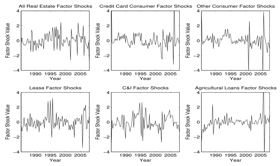
and the shocks should follow a white noise process. Inspection suggests that there\text{and the shocks should follow a white noise process. Inspection suggests that there}
Watson statistic tests for autocorrelation in the residuals of a regression. Table 2\text{Watson statistic tests for autocorrelation in the residuals of a regression. Table 2}
As additional specification tests, we perform normality tests on the innovations\text{As additional specification tests, we perform normality tests on the innovations}

All Real Estate Factor Shocks Credit Card Consumer Factor Shocks Other Consumer Factor Shocks 4 4 4

2 2 2

0 0 0 Factor Shock Value −2 Factor Shock Value −2 Factor Shock Value −2

−4 −4 −4 1990 1995 2000 2005 1990 1995 2000 2005 1990 1995 2000 2005 Year Year Year

Lease Factor Shocks C&I Factor Shocks Agricultural Loans Factor Shocks 4 4 4

2 2 2

Plots of the common factor autoregressive innovations extracted from the US banks aggregate quar-\text{Plots of the common factor autoregressive innovations extracted from the US banks aggregate quar-}
cant degree from their values under normality. We generate confidence levels for\text{cant degree from their values under normality. We generate confidence levels for}
The Durbin-Watson and the Jarque-Bera tests suggests no rejections of the null\text{The Durbin-Watson and the Jarque-Bera tests suggests no rejections of the null}
Figure 2
Autoregressive Factor Shocks Plots of the common factor autoregressive innovations extracted from the US banks aggregate quar- terly loan loss rates. The inferred shocks are from 1985 to fourth quarter 2007.

4.2 Factor Correlations

different sectors of the loan market will help a bank reduce its risk. In asking such\text{different sectors of the loan market will help a bank reduce its risk. In asking such}
factor innovations from the dynamic model, in both cases based on quarterly data.\text{factor innovations from the dynamic model, in both cases based on quarterly data.}

Table 2: Hypothesis Testing on the Autoregressive Shocks

the confidence level of 1.679 implies the null is not rejected at 95%. The Jarques-Bera test assesses\text{the confidence level of 1.679 implies the null is not rejected at 95\%. The Jarques-Bera test assesses}
RECCOCLCIADurbin-Watson2.292.342.572.231.892.54\begin{array}{lcccccc} & \text{RE} & \text{CC} & \text{OC} & \text{L} & \text{CI} & \text{A} \\ \text{Durbin-Watson} & 2.29 & 2.34 & 2.57 & 2.23 & 1.89 & 2.54 \end{array}
correlated with Other Consumer Loans. All Real Estate is fairly highly correlated\text{correlated with Other Consumer Loans. All Real Estate is fairly highly correlated}
Loans. This reflects the fact that the shocks in the static model may be thought\text{Loans. This reflects the fact that the shocks in the static model may be thought}
components (see Table 4). To analyze how far the correlation matrix is from one with\text{components (see Table 4). To analyze how far the correlation matrix is from one with}
factors are present in the factors driving the individual loan loss rates. More details\text{factors are present in the factors driving the individual loan loss rates. More details}
First the eigenvalues are arranged in ascending order. The smallest p eigenvalues\text{First the eigenvalues are arranged in ascending order. The smallest } p \text{ eigenvalues}

Table 3: Loss Rate Correlation Matrices

using quarterly US bank loss rates. In the static case the correlation between the common factors\text{using quarterly US bank loss rates. In the static case the correlation between the common factors}
A0.37−0.33−0.230.410.551.00Correlation Matrix with AutocorrelationRE1.00−0.180.110.160.280.40\begin{array}{lcccccc} \text{A} & 0.37 & -0.33 & -0.23 & 0.41 & 0.55 & 1.00 \\ \hline \text{Correlation Matrix with Autocorrelation} \\ \hline \text{RE} & 1.00 & -0.18 & 0.11 & 0.16 & 0.28 & 0.40 \end{array}
dence levels. The tests suggest that in both the static and dynamic model, multiple\text{dence levels. The tests suggest that in both the static and dynamic model, multiple}
most important. The corporate loan categories, C&I and Leases mainly have positive\text{most important. The corporate loan categories, C\&I and Leases mainly have positive}

Table 4: Principal Component Analysis of Factor Correlations

both a model with and without autocorrelation in the factor. Each row is an unobserved factor that\text{both a model with and without autocorrelation in the factor. Each row is an unobserved factor that}
Common Factor 62.600.29−0.09−0.020.300.350.28Eigenvalue and Factor Weights with AutocorrelationCommon Factor 10.410.61−0.760.33−0.14−0.26−1.15\begin{array}{lcccccc} \text{Common Factor 6} & 2.60 & 0.29 & -0.09 & -0.02 & 0.30 & 0.35 & 0.28 \\ \hline \text{Eigenvalue and Factor Weights with Autocorrelation} \\ \hline \text{Common Factor 1} & 0.41 & 0.61 & -0.76 & 0.33 & -0.14 & -0.26 & -1.15 \end{array}

5 Conditional Default Rate Distributions

5.1 Conditioning on Macroeconomic Variables

VaRs or Expected Shortfalls for the distribution of the future portfolio value. These\text{VaRs or Expected Shortfalls for the distribution of the future portfolio value. These}
growth). Such analysis is often referred to as stress testing. Research on stress\text{growth). Such analysis is often referred to as stress testing. Research on stress}

Table 5: Hypothesis Testing of Eigenvalues

lation matrix. Appendix A describes the testing hypothesis. Values at each of the confidence limits\text{lation matrix. Appendix A describes the testing hypothesis. Values at each of the confidence limits}
Confidence Limit75%85%90%95%Model with No Autocorrelation4332\begin{array}{lcccc} \text{Confidence Limit} & 75\% & 85\% & 90\% & 95\% \\ \hline \text{Model with No Autocorrelation} & 4 & 3 & 3 & 2 \end{array}
macroeconomic shocks and hence, in a sense, devise stress test methods for credit\text{macroeconomic shocks and hence, in a sense, devise stress test methods for credit}
Duffie, Saita, and Wang (2007) suppose that fluctuation in observable variables induce\text{Duffie, Saita, and Wang (2007) suppose that fluctuation in observable variables induce}
obligor i is assumed to default at time t based on equation (1). Now, suppose that\text{obligor } i \text{ is assumed to default at time } t \text{ based on equation (1). Now, suppose that}
factors:Zit=ρ(1−λ2Xt+λ∑j=1Jaj∗Yj,t)+1−ρ ϵi,t .\text{factors:} \qquad Z_{it} = \sqrt{\rho}\left(\sqrt{1-\lambda^{2}}X_t + \lambda\sum_{j=1}^{J} a_j^{*} Y_{j,t}\right) + \sqrt{1-\rho}\,\epsilon_{i,t}\ .
(35)
ηt are assumed to be independent standard normals. λ determines the contribution\eta_t \text{ are assumed to be independent standard normals. } \lambda \text{ determines the contribution}
term by redefining the observable factor weights as:\text{term by redefining the observable factor weights as:}
aj≡aj∗∑k=1J∑m=1JakamCovariance(Yk,t,Ym,t)a_j \equiv \frac{a_j^*}{\sqrt{\sum_{k=1}^{J}\sum_{m=1}^{J} a_k a_m \mathrm{Covariance}(Y_{k,t}, Y_{m,t})}}
(36)
and modifying the default driver of obligor i to:\text{and modifying the default driver of obligor } i \text{ to:}
Zit=ρ(1−λ2Xt+λa′Y)+1−ρ ϵi,t .Z_{it} = \sqrt{\rho}\left(\sqrt{1-\lambda^2}X_t + \lambda a'Y\right) + \sqrt{1-\rho}\,\epsilon_{i,t} \ .
(37)
weights are expressed as vectors. The Yj,t are assumed to be stationary series so the\text{weights are expressed as vectors. The } Y_{j,t} \text{ are assumed to be stationary series so the}
conomic factors closely follows that of Section 2. The loss rate distribution conditional\text{conomic factors closely follows that of Section 2. The loss rate distribution conditional}
W(θt)≡Φ(1−ρ Φ−1(θt)−Φ−1(q)+ρ1−λ2βXt−1+ρλaYρ1−λ21−β) .W(\theta_t) \equiv \Phi\left(\frac{\sqrt{1-\rho}\,\Phi^{-1}(\theta_t) - \Phi^{-1}(q) + \sqrt{\rho}\sqrt{1-\lambda^2}\sqrt{\beta}X_{t-1} + \sqrt{\rho}\lambda aY}{\sqrt{\rho}\sqrt{1-\lambda^2}\sqrt{1-\beta}}\right) \ .
(38)
distribution:\text{distribution:}
N(Φ−1(q)−ρ1−λ2βXt−1−ρλaY1−ρ, ρ(1−λ2)(1−β)1−ρ) .\mathrm{N}\left(\frac{\Phi^{-1}(q) - \sqrt{\rho}\sqrt{1-\lambda^2}\sqrt{\beta}X_{t-1} - \sqrt{\rho}\lambda aY}{\sqrt{1-\rho}}, \ \frac{\rho(1-\lambda^2)(1-\beta)}{1-\rho}\right) \ .
(39)
dard deviation and a shock. This can then be rearranged, lagged and substituted\text{dard deviation and a shock. This can then be rearranged, lagged and substituted}

Proposition 3 When individual-borrower latent variables, ZitZ_{it}, and the unobserved common factor XtX_t, follow the processes given by equations (35)and (5), respectively, as the number of loans n→∞n \to \infty, the transformed loss rate, θ~t≡Φ−1(θt)\tilde{\theta}_t \equiv \Phi^{-1}(\theta_t) , converges to the process

θ~t=βθ~t−1+1−β1−ρΦ−1(q)\tilde{\theta}_t = \sqrt{\beta}\tilde{\theta}_{t-1} + \frac{1-\sqrt{\beta}}{\sqrt{1-\rho}}\Phi^{-1}(q)
−ρ1−ρλa(Yt−βYt−1)−ρ1−λ21−ρ1−βηt .-\frac{\sqrt{\rho}}{\sqrt{1-\rho}}\lambda a(Y_t - \sqrt{\beta}Y_{t-1}) - \frac{\sqrt{\rho}\sqrt{1-\lambda^2}}{\sqrt{1-\rho}}\sqrt{1-\beta}\eta_t \ .
(40)

Unemployment Rate

Percent (%)

1950 1960 1970 1980 1990 2000 Year

Industrial Production

Index based (2002 = 100) 20

1920 1930 1940 1950 1960 1970 1980 1990 2000 Year

Figure 3: Macro-Economic Stress Parameters

is the US Unemployment Rate over the period 1948 to 2007 and the lower panel is the US Industrial\text{is the US Unemployment Rate over the period 1948 to 2007 and the lower panel is the US Industrial}

5.2 Estimation

described: Credit Card losses and C&I losses. As before, the series were re-scaled by\text{described: Credit Card losses and C\&I losses. As before, the series were re-scaled by}
stresses involving the US Employment Rate and US Industrial Production.2 The\text{stresses involving the US Employment Rate and US Industrial Production.}^{2}\text{ The}
changes in unemployment and growth in production so we expressed the two series as\text{changes in unemployment and growth in production so we expressed the two series as}

Industrial Production Annual % Change

−1

−2

−3

−4 1986 1988 1990 1992 1994 1996 1998 2000 2002 2004 2006 2008 Year

Unemployment Rate Annual % Change

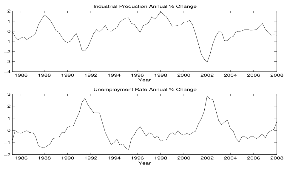
same period as the loss rate data, 1985 to 2007, and both series have been transformed to standard\text{same period as the loss rate data, 1985 to 2007, and both series have been transformed to standard}
dividing by their sample standard deviations. Figure 4 shows the normalised series\text{dividing by their sample standard deviations. Figure 4 shows the normalised series}
ployed Maximum Likelihood. In a multivariate setting the weights on the observed\text{ployed Maximum Likelihood. In a multivariate setting the weights on the observed}
Figure 4
Normalised Stress Series Stress series used as observable conditioning variables in the model. The series are both over the same period as the loss rate data, 1985 to 2007, and both series have been transformed to standard normal. The top panel is the annual percentage change in US Employment Rate and the lower panel is the annual percentage change in US Industrial Production.

5.3 Stress Estimates

the annual percentage change in the US Unemployment Rate, (ii) the C&I loss rate\text{the annual percentage change in the US Unemployment Rate, (ii) the C\&I loss rate}
For the Credit Card losses, the factor correlation, ρ, is 0.60%. The unconditional\text{For the Credit Card losses, the factor correlation, } \rho \text{, is } 0.60\%\text{. The unconditional}

Table 6: Univariate Stress Parameterisation

US Unemployment Rate over the period 1985 to 2007. The values in parenthesis are the t-statistics\text{US Unemployment Rate over the period 1985 to 2007. The values in parenthesis are the t-statistics}
Factor correlation ρ (%)0.60\text{Factor correlation } \rho\ (\%) \quad 0.60
(3.83)
Unconditional default probability q (%)1.67\text{Unconditional default probability q } (\%) \quad 1.67
(16.15)
AR(1) parameter β (%)68.14\text{AR(1) parameter } \beta\ (\%) \quad 68.14
(8.32)
Stress coefficient λ (%)−37.56(−2.88)−26.22(−2.34)\text{Stress coefficient } \lambda\ (\%) \quad -37.56 \quad (-2.88) \quad -26.22 \quad (-2.34)
coefficient is correct. The stress coefficient is negative. This means that as the Unem-\text{coefficient is correct. The stress coefficient is negative. This means that as the Unem-}
much lower at 0.38% while the factor reversion is higher at 89.58%. Again, the\text{much lower at } 0.38\% \text{ while the factor reversion is higher at } 89.58\%\text{. Again, the}
dynamic model. The parameters estimates are all slightly smaller. The correlation\text{dynamic model. The parameters estimates are all slightly smaller. The correlation}
EquationEquationEquation

Table 7: Multivariate Stress Parameterisation

EquationEquation (1.94)Equation (3.01)EquationEquation (0.56)Equation

5.4 Stressed Default Rate Distributions

Equation
Unemployment Rate stress, Figure 5, one can see how the loss rates are driven by\text{Unemployment Rate stress, Figure 5, one can see how the loss rates are driven by}
Table 8 shows statistics for these distributions. Looking first at the four year hori-\text{Table 8 shows statistics for these distributions. Looking first at the four year hori-}
The one-year horizon loss rates present a different picture. Note that in Figure 5,\text{The one-year horizon loss rates present a different picture. Note that in Figure 5,}
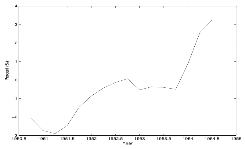
employment Rate. Stress period found to be 1950 to 1954. The series has been transformed to\text{employment Rate. Stress period found to be 1950 to 1954. The series has been transformed to}
case is higher, at 1.81%, than the unconditional case, at 1.69%. But, due to the drop\text{case is higher, at 1.81\%, than the unconditional case, at 1.69\%. But, due to the drop}
Figure 5
Unemployment Recession Stress The four year period of maximum positive change in the annual percentage differences in US Un- employment Rate. Stress period found to be 1950 to 1954. The series has been transformed to standard normal using the same normalisation parameters as those in the estimation exercise.

6 Capital Implications

6.1 Implied Capital

Marginal Value at Risk (MVaRα) for a single loan may be calculated as the expected\text{Marginal Value at Risk (MVaR}_{\alpha}\text{) for a single loan may be calculated as the expected}
MVaRα=LGD×Φ(Φ−1(q)−ρβXt−1−ρ1−βΦ−1(α)1−ρ) ,\mathrm{MVaR}_{\alpha} = \mathrm{LGD} \times \Phi\left(\frac{\Phi^{-1}(q) - \sqrt{\rho}\sqrt{\beta}X_{t-1} - \sqrt{\rho}\sqrt{1-\beta}\Phi^{-1}(\alpha)}{\sqrt{1-\rho}}\right) \ ,
(41)

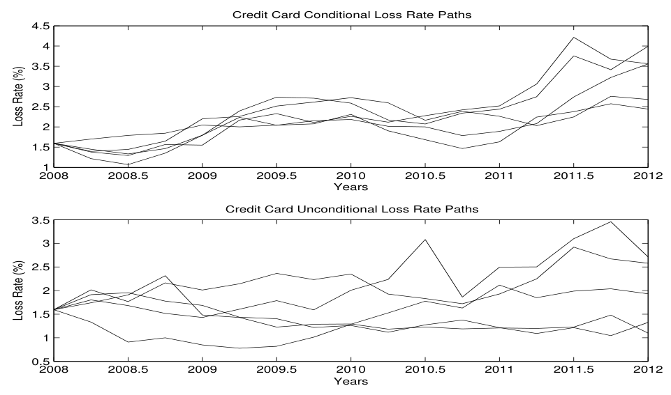
Credit Card Conditional Loss Rate Paths 4.5

3.5

2.5 Loss Rate (%) 2 1.5

2008 2008.5 2009 2009.5 2010 2010.5 2011 2011.5 2012 Years

Credit Card Unconditional Loss Rate Paths 3.5

2.5 Loss Rate (%) 1.5

Credit Card loss rates stressing on the annual percentage change in US Unemployment Rate between\text{Credit Card loss rates stressing on the annual percentage change in US Unemployment Rate between}
where the factor shock, ηt is taken at its α-quantile.\text{where the factor shock, } \eta_t \text{ is taken at its } \alpha\text{-quantile.}
The probability of default conditional on information at t−1 is given by equation\text{The probability of default conditional on information at } t-1 \text{ is given by equation}

Proposition 4 Under the above assumptions, the Marginal Value at Risk for a single loan, denoted MVaRα\mathrm{MVaR}_\alpha, is:

MVaRα=LGD×Φ(1−ρβΦ−1(qt)−ρ1−βΦ−1(α)1−ρ) .\mathrm{MVaR}_{\alpha} = \mathrm{LGD} \times \Phi\left(\sqrt{1-\rho\beta}\frac{\Phi^{-1}(q_t) - \sqrt{\rho}\sqrt{1-\beta}\Phi^{-1}(\alpha)}{\sqrt{1-\rho}}\right) \ .
(42)
the expected loss:\text{the expected loss:}
Basel Capital Formula=LGD×Φ(Φ−1(q)+ρ1−βΦ−1(α∗)1−ρ)−LGD\text{Basel Capital Formula} = \mathrm{LGD} \times \Phi\left(\frac{\Phi^{-1}(q) + \sqrt{\rho}\sqrt{1-\beta}\Phi^{-1}(\alpha^{*})}{\sqrt{1-\rho}}\right) - \mathrm{LGD}
(43)
default probability qt. When β=0 so the factor is no longer autocorrelated, the\text{default probability } q_t. \text{ When } \beta = 0 \text{ so the factor is no longer autocorrelated, the}

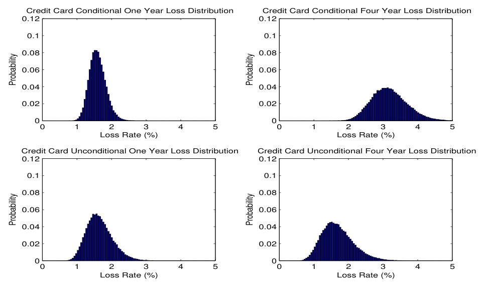
Credit Card Conditional One Year Loss Distribution Credit Card Conditional Four Year Loss Distribution 0.12 0.12

0.1 0.1

0.08 0.08

0.06 0.06 Probability Probability 0.04 0.04

0.02 0.02

0 0 0 1 2 3 4 5 0 1 2 3 4 5 Loss Rate (%) Loss Rate (%)

Credit Card Unconditional One Year Loss Distribution Credit Card Unconditional Four Year Loss Distribution 0.12 0.12

0.1 0.1

One and four year conditional and unconditional simulated loss distributions of US Credit Card loss\text{One and four year conditional and unconditional simulated loss distributions of US Credit Card loss}
Figure 6
Stress Monte Carlo Paths Example loss rate paths over a four year period for the conditional and unconditional cases of US Credit Card loss rates stressing on the annual percentage change in US Unemployment Rate between 1950-1954.
Figure 7
Stressed Loss Distributions One and four year conditional and unconditional simulated loss distributions of US Credit Card loss rates stressing on the annual percentage change in US Unemployment Rate between 1950-1954.

6.2 Regulatory Implications

banks if the data period is one year. We therefore convert the data from quarterly\text{banks if the data period is one year. We therefore convert the data from quarterly}
assumes a point-in-time default probability as a parameter for their formulae. We\text{assumes a point-in-time default probability as a parameter for their formulae. We}
that the capital implied by the autocorrelation case is less than the static case for all\text{that the capital implied by the autocorrelation case is less than the static case for all}

Table 8: Stressed Loss Distribution Statistics

stressed. In the conditional case the annual percentage differences in US Unemployment Rate over\text{stressed. In the conditional case the annual percentage differences in US Unemployment Rate over}
Year 1Year 4Year 1Year 4Mean1.813.191.661.69\begin{array}{lcccc} & \text{Year 1} & \text{Year 4} & \text{Year 1} & \text{Year 4} \\ \hline \text{Mean} & 1.81 & 3.19 & 1.66 & 1.69 \end{array}
As an example, the other consumer category implies 1.11% using the autocorrelation\text{As an example, the other consumer category implies 1.11\% using the autocorrelation}
formulae are just convenient functions that happens to have the right shape.) But\text{formulae are just convenient functions that happens to have the right shape.) But}

7 Conclusion

Our generalization allows for the dynamic evolution of loan loss distributions. Intro-\text{Our generalization allows for the dynamic evolution of loan loss distributions. Intro-}
risk at an aggregate level. The results show that the risk characteristics and general\text{risk at an aggregate level. The results show that the risk characteristics and general}

Table 9: Capital Calculations

period. The capital is calculated using equation (42). The common parameterisation is shown in\text{period. The capital is calculated using equation (42). The common parameterisation is shown in}
With no autocorrelation10.531.311.335.167.2513.98\text{With no autocorrelation} \quad 10.53 \quad 1.31 \quad 1.33 \quad 5.16 \quad 7.25 \quad 13.98
this model. This can help banks or other financial institutions analyse their risks in\text{this model. This can help banks or other financial institutions analyse their risks in}

Appendix

A Eigenvalue Tests for a Covariance Matrix

composition of a covariance matrix. The testing hypothesis is taken from Anderson\text{composition of a covariance matrix. The testing hypothesis is taken from Anderson}
matrix are small compared to the sum of all the roots of the covariance matrix. A\text{matrix are small compared to the sum of all the roots of the covariance matrix. A}
H:f(λ)=λm+1+⋅+λp(λ1+⋯+λp)2≥δ,H : f(\lambda) = \frac{\lambda_{m+1} + \cdot + \lambda_p}{(\lambda_1 + \cdots + \lambda_p)^2} \geq \delta,
(A1)
where δ is a specified confidence level, could then be defined to reject the hypothesis\text{where } \delta \text{ is a specified confidence level, could then be defined to reject the hypothesis}
The null is then rejected if:\text{The null is then rejected if:}
n(f(λ)−δ)≤Φ−1(1−δ)σλ,\sqrt{n}(f(\lambda) - \delta) \leq \Phi^{-1}(1-\delta)\sigma_\lambda,
(A2)
where Φ is the standard normal cdf and the variance of f(λ) is given by:\text{where } \Phi \text{ is the standard normal cdf and the variance of } f(\lambda) \text{ is given by:}
σλ2=2(δ∑i=1pλi)2∑i=1mλi2+2(1−δ∑i=1pλi)2∑i=m+1pλi2.\sigma_\lambda^2 = 2\left(\frac{\delta}{\sum_{i=1}^p \lambda_i}\right)^2 \sum_{i=1}^m \lambda_i^2 + 2\left(1 - \frac{\delta}{\sum_{i=1}^p \lambda_i}\right)^2 \sum_{i=m+1}^p \lambda_i^2.
(A3)

References

Altman, E. I. (1968): “Financial Ratios, Discriminant Analysis, and the Prediction\text{Altman, E. I. (1968): ``Financial Ratios, Discriminant Analysis, and the Prediction}
Anderson, T. W. (2003): An Introduction to Multivariate Statistical Analysis.\text{Anderson, T. W. (2003): } \textit{An Introduction to Multivariate Statistical Analysis.}
atic Risk in the International Financial System,” Journal of Financial Economics,\text{atic Risk in the International Financial System,''} \textit{ Journal of Financial Economics,}
Basel Committee on Banking Supervision (1999): “A New Capital Adequacy\text{Basel Committee on Banking Supervision (1999): ``A New Capital Adequacy}
Becker, B. (2007): “Geographical Segmentation of US Capital Markets,” Journal\text{Becker, B. (2007): ``Geographical Segmentation of US Capital Markets,''} \textit{ Journal}
Berkowitz, J. (1999): “A Coherent Framework for Stress-Testing,” Journal of Risk,\text{Berkowitz, J. (1999): ``A Coherent Framework for Stress-Testing,'' \textit{Journal of Risk},}
Carey, M. (1998): “Credit Risk in Private Debt Portfolios,” Journal of Finance,\text{Carey, M. (1998): ``Credit Risk in Private Debt Portfolios,'' \textit{Journal of Finance},}
Chava, S., and R. Jarrow (2004): “Bankruptcy Prediction with Industry Effects,”\text{Chava, S., and R. Jarrow (2004): ``Bankruptcy Prediction with Industry Effects,''}
Couderc, F., and O. Renault (2004): “Times-to-Default: Life Cycle, Global and\text{Couderc, F., and O. Renault (2004): ``Times-to-Default: Life Cycle, Global and}
Das, S. R., D. Duffie, N. Kapadia, and L. Saita (2007): “Common Failings:\text{Das, S. R., D. Duffie, N. Kapadia, and L. Saita (2007): ``Common Failings:}
de Servigny, A., and O. Renault (2002): “Default Correlation: Empirical Evi-\text{de Servigny, A., and O. Renault (2002): ``Default Correlation: Empirical Evi-}
Duffie, D., A. Eckner, G. Horel, and L. Saita (2006): “Frailty Correlated\text{Duffie, D., A. Eckner, G. Horel, and L. Saita (2006): ``Frailty Correlated}
Prediction with Stochastic Covariates,” Journal of Financial Economics, 83(3),\text{Prediction with Stochastic Covariates,'' \textit{Journal of Financial Economics}, 83(3),}
Gordy, M. (2003): “A Risk-Factor Model Foundation for Ratings-Based Bank Cap-\text{Gordy, M. (2003): ``A Risk-Factor Model Foundation for Ratings-Based Bank Cap-}
Gross, D. B., and N. S. Souleles (2002): “An Empirical Analysis of Personal\text{Gross, D. B., and N. S. Souleles (2002): ``An Empirical Analysis of Personal}
Hamilton, J. D. (1994): Times Series Analysis. Princeton University Press, Prince-\text{Hamilton, J. D. (1994): } \textit{Times Series Analysis}\text{. Princeton University Press, Prince-}
“Assessing the Probability of Bankruptcy,” Review of Accounting Studies, 9(1), 5–\text{``Assessing the Probability of Bankruptcy,'' } \textit{Review of Accounting Studies}\text{, 9(1), 5--}
Kealhofer, S. (2003): “Quantifying Credit Risk I: Default Prediction,” Financial\text{Kealhofer, S. (2003): ``Quantifying Credit Risk I: Default Prediction,'' } \textit{Financial}
Koopman, S. J., and A. Lucas (2005): “Business and default cycles for credit\text{Koopman, S. J., and A. Lucas (2005): ``Business and default cycles for credit}
Koopman, S. J., A. Lucas, and P. Klaassen (2005): “Empirical credit cycles\text{Koopman, S. J., A. Lucas, and P. Klaassen (2005): ``Empirical credit cycles}
Kupiec, P. (1998): “Stress Testing in a Value at Risk Framework,” Journal of\text{Kupiec, P. (1998): ``Stress Testing in a Value at Risk Framework,'' } \textit{Journal of}
Drift with Continuous Observations,” Journal of Banking and Finance, 26(2-3),\text{Drift with Continuous Observations,'' } \textit{Journal of Banking and Finance}\text{, 26(2-3),}
the Cox Proportional Hazards Model to Bank Failure,” Journal of Banking and\text{the Cox Proportional Hazards Model to Bank Failure,'' } \textit{Journal of Banking and}
in the Property-Liability Insurance Industry: A Comparison of Logit and Hazard\text{in the Property-Liability Insurance Industry: A Comparison of Logit and Hazard}
Longin, F. (2000): “From Value at Risk to Stress Testing: The Extreme Value\text{Longin, F. (2000): ``From Value at Risk to Stress Testing: The Extreme Value}
McNeil, A. J. M., and J. Wendin (2006): “Dependent Credit Migrations,” Work-\text{McNeil, A. J. M., and J. Wendin (2006): ``Dependent Credit Migrations,'' Work-}
——- (2007): “Bayesian Inference for Generalized Linear Mixed Models of Port-\text{------- (2007): ``Bayesian Inference for Generalized Linear Mixed Models of Port-}
Nickell, P., W. R. Perraudin, and S. Varotto (2000): “The Stability of\text{Nickell, P., W. R. Perraudin, and S. Varotto (2000): ``The Stability of}
Ohlson, J. A. (1980): “Financial Ratios and the Probabilistic Prediction of\text{Ohlson, J. A. (1980): ``Financial Ratios and the Probabilistic Prediction of}

Pesaran, M., T. Schuermann, B. Treutler, and S. Weiner (2006): “Macroeconomic Dynamics and Credit Risk: A Global Perspective,” Journal of Money, Credit and Banking, 38(5), 1211–1261.

Pesaran, M., T. Schuermann, and S. Weiner (2004): “Modeling Regional Interdependencies Using a Global Error-Correcting Macroeconomic Model,” Journal of Business and Economic Statistics, 22, 129–162.

Peura, S., and E. Jokivuolle (2004): “Simulation-based stress testing of banks\text{Peura, S., and E. Jokivuolle (2004): ``Simulation-based stress testing of banks}
tegrated Risk Management with Skewed, Fat-Tailed Risks,” Journal of Financial\text{tegrated Risk Management with Skewed, Fat-Tailed Risks,'' \textit{Journal of Financial}}
Ruckes, M. (2004): “Bank Competition and Credit Standards,” The Review of\text{Ruckes, M. (2004): ``Bank Competition and Credit Standards,'' \textit{The Review of}}
Schonbucher, P. J. (2002): “Taken to the Limit: Simple and Not So Simple Loan\text{Schonbucher, P. J. (2002): ``Taken to the Limit: Simple and Not So Simple Loan}
Schumway, T. (2001): “Forecasting Bankruptcy More Accurately: A Simple Hazard\text{Schumway, T. (2001): ``Forecasting Bankruptcy More Accurately: A Simple Hazard}
Vasicek, O. (1991): “Limiting Loan Loss Probability Distribution,” Unpublished\text{Vasicek, O. (1991): ``Limiting Loan Loss Probability Distribution,'' Unpublished}
Zhou, C. (2001): “The term structure of credit spreads with jump risk,” Journal of\text{Zhou, C. (2001): ``The term structure of credit spreads with jump risk,'' \textit{Journal of}}

Notes

∗The authors’ may be contacted at [email protected] or [email protected]. An earlier version of this paper was circulated under the title ‘Dynamic Loan Loss Distributions: Esti- mation and Implications’. 1An initial value of X[0] = 0 was assumed for each factor series. 2Das, Duffie, Kapadia, and Saita (2007) find some evidence that growth in US Industrial Pro- duction explains covariation in individual borrower default rates. 3We performed Dicky-Fuller tests on the stress series, not reported here, that confirmed the series are stationary.

100%