This paper applies a new class of dynamic credit loss rate models to the pricing of benchmark synthetic Collateralized Debt Obligations (CDOs). Our approach builds directly on the static, industry-standard, pricing approach to credit structured products based on Vasicek (1991). We generalize the Vasicek model by allowing risk factors to be driven by arbitrarily complex autoregressive processes. We show how to benchmark our model using CDX prices, and demonstrate that it can consistently and accurately fit the prices of multiple tranches with different subordination levels and tenors. Among other interesting results, we find that changes in tranche spreads are driven less by alterations in the market’s estimate of default correlation (which is stable over time) and more by fluctuations in market perceptions of the persistence of credit shocks, i.e., the persistence of the credit cycle.
1 Introduction These authors generated correlated intensities using affine processes for individual \text{These authors generated correlated intensities using affine processes for individual} These authors generated correlated intensities using affine processes for individual develop an intensity based approach to modeling total portfolio losses, inferring single \text{develop an intensity based approach to modeling total portfolio losses, inferring single} develop an intensity based approach to modeling total portfolio losses, inferring single approaches modeling evolution of the losses on a portfolio. Sidenius, Piterbarg, and \text{approaches modeling evolution of the losses on a portfolio. Sidenius, Piterbarg, and} approaches modeling evolution of the losses on a portfolio. Sidenius, Piterbarg, and tion to the market is performed by conditioning upon a background process. The \text{tion to the market is performed by conditioning upon a background process. The} tion to the market is performed by conditioning upon a background process. The Pallavicini, and Torresetti (2007) assumes the loss process is a sum of independent \text{Pallavicini, and Torresetti (2007) assumes the loss process is a sum of independent} Pallavicini, and Torresetti (2007) assumes the loss process is a sum of independent series process. They derive a closed form expression for a simple transformation of \text{series process. They derive a closed form expression for a simple transformation of} series process. They derive a closed form expression for a simple transformation of to pricing synthetic CDOs. Though we focus here on synthetic CDOs, a type of struc- \text{to pricing synthetic CDOs. Though we focus here on synthetic CDOs, a type of struc-} to pricing synthetic CDOs. Though we focus here on synthetic CDOs, a type of struc- We show how the distribution of losses at future dates is affected by conditioning \text{We show how the distribution of losses at future dates is affected by conditioning} We show how the distribution of losses at future dates is affected by conditioning 2.1 Loss Rate Process Suppose that time is discrete taking values t = 0 , 1 , … and that there are n obligors \text{Suppose that time is discrete taking values } t = 0, 1, \ldots \text{ and that there are n obligors} Suppose that time is discrete taking values t = 0 , 1 , … and that there are n obligors Z i , t ≤ c t Z_{i,t} \leq c_t Z i , t ≤ c t (1) into the model by defining Z i , t to be a latent random variable such that: \text{into the model by defining } Z_{i,t} \text{ to be a latent random variable such that:} into the model by defining Z i , t to be a latent random variable such that: Z i , t = ρ X t + 1 − ρ ϵ i , t . Z_{i,t} = \sqrt{\rho} X_t + \sqrt{1-\rho}\epsilon_{i,t}. Z i , t = ρ X t + 1 − ρ ϵ i , t . (2) specific idiosyncratic shock, ϵ i , t , has a distribution function H , a zero mean and unit \text{specific idiosyncratic shock, } \epsilon_{i,t}, \text{ has a distribution function } H, \text{ a zero mean and unit} specific idiosyncratic shock, ϵ i , t , has a distribution function H , a zero mean and unit a standard normal distribution function Φ . G depends on ρ and on a vector of \text{a standard normal distribution function } \Phi. \ G \text{ depends on } \rho \text{ and on a vector of} a standard normal distribution function Φ. G depends on ρ and on a vector of G ( z ) = ∫ − ∞ ∞ H ( z − ρ x 1 − ρ ) d Φ ( x ) . G(z) = \int_{-\infty}^{\infty} H\left(\frac{z - \sqrt{\rho}x}{\sqrt{1-\rho}}\right) d\Phi(x) \ . G ( z ) = ∫ − ∞ ∞ H ( 1 − ρ z − ρ x ) d Φ ( x ) . (3) Given this distribution, one may express the unconditional probability that default \text{Given this distribution, one may express the unconditional probability that default} Given this distribution, one may express the unconditional probability that default q t = P r o b ( d e f a u l t a t t ) = G ( c t ) . q_t = \mathrm{Prob}\left(\mathrm{default\ at\ } t\right) \ = \ G\left(c_t\right). q t = Prob ( default at t ) = G ( c t ) . (4) introduce dynamics, we follow Lamb and Perraudin (2006) by allowing X i , t to be a \text{introduce dynamics, we follow Lamb and Perraudin (2006) by allowing } X_{i,t} \text{ to be a} introduce dynamics, we follow Lamb and Perraudin (2006) by allowing X i , t to be a X t = ∑ i = 1 p ϕ i X t − i + σ η t . X_t = \sum_{i=1}^{p} \phi_i X_{t-i} + \sigma \eta_t. X t = i = 1 ∑ p ϕ i X t − i + σ η t . (5) Here, η t is assumed to be standard normal and independent of ϵ i , t . \text{Here, } \eta_t \text{ is assumed to be standard normal and independent of } \epsilon_{i,t}. Here, η t is assumed to be standard normal and independent of ϵ i , t . Substitution of equation (2) into (1) shows that default occurs when : \text{Substitution of equation (2) into (1) shows that default occurs when :} Substitution of equation (2) into (1) shows that default occurs when : P ( k , n ) , may be expressed as: P(k,n), \text{ may be expressed as:} P ( k , n ) , may be expressed as: Adopting the change of variables: \text{Adopting the change of variables:} Adopting the change of variables: 
for the fraction of the pool that defaults denoted θ : \text{for the fraction of the pool that defaults denoted } \theta: for the fraction of the pool that defaults denoted θ : Z[1] = 1(s < θ)dW (s) = W (θ) − W (0) = W (θ) . (12)
Hence, the loss distribution conditional on X t − 1 is: \text{Hence, the loss distribution conditional on } X_{t-1} \text{ is:} Hence, the loss distribution conditional on X t − 1 is: 
θ ~ t ≡ H − 1 ( θ t ) ∼ N ( c t − ρ ∑ i = 1 p ϕ i X t − i 1 − ρ , σ 2 ρ 1 − ρ ) . \tilde{\theta}_t \equiv H^{-1}(\theta_t) \sim \mathrm{N}\left(\frac{c_t - \sqrt{\rho}\sum_{i=1}^{p} \phi_i X_{t-i}}{\sqrt{1-\rho}},\ \frac{\sigma^2 \rho}{1-\rho}\right). θ ~ t ≡ H − 1 ( θ t ) ∼ N ( 1 − ρ c t − ρ ∑ i = 1 p ϕ i X t − i , 1 − ρ σ 2 ρ ) . (14) θ ~ t = c t − ρ ∑ i = 1 p ϕ i X t − i 1 − ρ − σ ρ 1 − ρ η t . \tilde{\theta}_t = \frac{c_t - \sqrt{\rho}\sum_{i=1}^{p} \phi_i X_{t-i}}{\sqrt{1-\rho}} - \frac{\sigma\sqrt{\rho}}{\sqrt{1-\rho}}\eta_t. θ ~ t = 1 − ρ c t − ρ ∑ i = 1 p ϕ i X t − i − 1 − ρ σ ρ η t . (15) θ ~ t = c t − ρ X t 1 − ρ . \tilde{\theta}_t = \frac{c_t - \sqrt{\rho}X_t}{\sqrt{1-\rho}} \ . θ ~ t = 1 − ρ c t − ρ X t . (16) θ ~ t = ∑ i = 1 p ϕ i θ ~ t − i + 1 1 − ρ ( c t − ∑ i = 1 p ϕ i c t − i ) − σ ρ 1 − ρ η t . \tilde{\theta}_t = \sum_{i=1}^{p} \phi_i \tilde{\theta}_{t-i} + \frac{1}{\sqrt{1-\rho}}\left(c_t - \sum_{i=1}^{p} \phi_i c_{t-i}\right) - \frac{\sigma\sqrt{\rho}}{\sqrt{1-\rho}}\eta_t. θ ~ t = i = 1 ∑ p ϕ i θ ~ t − i + 1 − ρ 1 ( c t − i = 1 ∑ p ϕ i c t − i ) − 1 − ρ σ ρ η t . (17) 2.2 Conditional Loss Distributions X ‾ t = F X ‾ t − 1 + σ ν ‾ t . \overline{X}_t = F\overline{X}_{t-1} + \sigma\overline{\nu}_t. X t = F X t − 1 + σ ν t . (18) where X ‾ t ≡ ( X t , X t − 1 , … , X t − p + 1 ) ′ and η ‾ t ≡ ( η t , 0 , … , 0 ) ′ and where F is defined in \text{where } \overline{X}_t \equiv (X_t, X_{t-1}, \ldots, X_{t-p+1})' \text{ and } \overline{\eta}_t \equiv (\eta_t, 0, \ldots, 0)' \text{ and where } F \text{ is defined in} where X t ≡ ( X t , X t − 1 , … , X t − p + 1 ) ′ and η t ≡ ( η t , 0 , … , 0 ) ′ and where F is defined in Recursive substitution of this to time t leads to: \text{Recursive substitution of this to time } t \text{ leads to:} Recursive substitution of this to time t leads to: or in matrix form: \text{or in matrix form:} or in matrix form: The first row of this system gives X t in terms of the factor values up to and including \text{The first row of this system gives } X_t \text{ in terms of the factor values up to and including} The first row of this system gives X t in terms of the factor values up to and including where f 1 , i ( t ) is the ( 1 , i ) element of F t . \text{where } f_{1,i}^{(t)} \text{ is the } (1,i) \text{ element of } F^t. where f 1 , i ( t ) is the ( 1 , i ) element of F t . time t is driven by the initial factor values and the compounded shocks: \text{time } t \text{ is driven by the initial factor values and the compounded shocks:} time t is driven by the initial factor values and the compounded shocks: ρ ( ∑ i = 1 p f 1 , i ( t ) X 1 − i + σ ∑ j = 0 t − 1 f 1 , 1 ( j ) η t − j ) + 1 − ρ ϵ i , t ≤ c t . \sqrt{\rho}\left(\sum_{i=1}^{p} f_{1,i}^{(t)} X_{1-i} + \sigma \sum_{j=0}^{t-1} f_{1,1}^{(j)} \eta_{t-j}\right) + \sqrt{1-\rho}\epsilon_{i,t} \leq c_t. ρ ( i = 1 ∑ p f 1 , i ( t ) X 1 − i + σ j = 0 ∑ t − 1 f 1 , 1 ( j ) η t − j ) + 1 − ρ ϵ i , t ≤ c t . (22) By conditioning on the information at time 0, we show how the distribution of the \text{By conditioning on the information at time 0, we show how the distribution of the} By conditioning on the information at time 0, we show how the distribution of the ρ σ ∑ j = 0 t − 1 f 1 , 1 ( j ) η t − j + 1 − ρ ϵ i , t ≤ c t − ρ ∑ i = 1 p f 1 , i ( t ) X 1 − i . \sqrt{\rho}\sigma \sum_{j=0}^{t-1} f_{1,1}^{(j)} \eta_{t-j} + \sqrt{1-\rho}\epsilon_{i,t} \leq c_t - \sqrt{\rho}\sum_{i=1}^{p} f_{1,i}^{(t)} X_{1-i}. ρ σ j = 0 ∑ t − 1 f 1 , 1 ( j ) η t − j + 1 − ρ ϵ i , t ≤ c t − ρ i = 1 ∑ p f 1 , i ( t ) X 1 − i . (23) Defining: c 0 , t = c t − ρ ∑ i = 1 p f 1 , i ( t ) X 1 − i , \text{Defining:}\quad c_{0,t} = c_t - \sqrt{\rho}\sum_{i=1}^{p} f_{1,i}^{(t)} X_{1-i}, Defining: c 0 , t = c t − ρ i = 1 ∑ p f 1 , i ( t ) X 1 − i , (24) gives: ρ σ ∑ j = 0 t − 1 f 1 , 1 ( j ) η t − j + 1 − ρ ϵ i , t ≤ c 0 , t , \text{gives:}\quad \sqrt{\rho}\sigma \sum_{j=0}^{t-1} f_{1,1}^{(j)} \eta_{t-j} + \sqrt{1-\rho}\epsilon_{i,t} \leq c_{0,t}, gives: ρ σ j = 0 ∑ t − 1 f 1 , 1 ( j ) η t − j + 1 − ρ ϵ i , t ≤ c 0 , t , (25) where G 0 , T is the convolution of : \text{where } G_{0,T} \text{ is the convolution of :} where G 0 , T is the convolution of : Φ ( x ρ σ 2 ∑ j = 0 t − 1 ( f 1 , 1 ( j ) ) 2 ) and H ( ν 1 − ρ ) . \Phi\left(\frac{x}{\sqrt{\rho\sigma^{2}\sum_{j=0}^{t-1}\left(f_{1,1}^{(j)}\right)^{2}}}\right) \quad \text{and} \quad H\left(\frac{\nu}{\sqrt{1-\rho}}\right)\ . Φ ρ σ 2 ∑ j = 0 t − 1 ( f 1 , 1 ( j ) ) 2 x and H ( 1 − ρ ν ) . (26) a single name is now: \text{a single name is now:} a single name is now: q 0 , t = G 0 , t ( c 0 , t ) . q_{0,t}=G_{0,t}\left(c_{0,t}\right). q 0 , t = G 0 , t ( c 0 , t ) . (27) Rearranging this equation shows how the default quantile c t is altered by the condi- \text{Rearranging this equation shows how the default quantile } c_{t} \text{ is altered by the condi-} Rearranging this equation shows how the default quantile c t is altered by the condi- tioning information: c t = G 0 , t − 1 ( q 0 , t ) + ρ ∑ i = 1 p f 1 , i ( t ) X 1 − i . \text{tioning information:} \quad c_{t}=G_{0,t}^{-1}\left(q_{0,t}\right)+\sqrt{\rho}\sum_{i=1}^{p}f_{1,i}^{(t)}X_{1-i}. tioning information: c t = G 0 , t − 1 ( q 0 , t ) + ρ i = 1 ∑ p f 1 , i ( t ) X 1 − i . (28) the default quantile from its unconditional case. As t → ∞ the term containing the \text{the default quantile from its unconditional case. As } t \rightarrow \infty \text{ the term containing the} the default quantile from its unconditional case. As t → ∞ the term containing the lim t → ∞ σ 2 ∑ j = 0 t − 1 ( f 1 , 1 ( j ) ) 2 → 1 lim t → ∞ G 0 , t ( z ) → G ( z ) . \lim_{t\to\infty}\sigma^{2}\sum_{j=0}^{t-1}\left(f_{1,1}^{(j)}\right)^{2}\to 1 \qquad \lim_{t\to\infty}G_{0,t}(z)\to G(z)\ . t → ∞ lim σ 2 j = 0 ∑ t − 1 ( f 1 , 1 ( j ) ) 2 → 1 t → ∞ lim G 0 , t ( z ) → G ( z ) . (29) 3.1 Tranche Valuation in equation (17), and then calculate the cumulative loss to the pool in each future \text{in equation (17), and then calculate the cumulative loss to the pool in each future} in equation (17), and then calculate the cumulative loss to the pool in each future L t = 1 − ∏ i = 1 t ( 1 − θ i ) . L_{t}=1-\prod_{i=1}^{t}\left(1-\theta_{i}\right)\ . L t = 1 − i = 1 ∏ t ( 1 − θ i ) . (30) If the pool has been tranched in a particular way to create levels of subordination, \text{If the pool has been tranched in a particular way to create levels of subordination,} If the pool has been tranched in a particular way to create levels of subordination, L t , j t r = min ( max ( ( 1 − γ ) L t − A 1 , j , 0 ) , A 2 , j − A 1 , j ) , L_{t,j}^{tr}=\min\left(\max\left(\left(1-\gamma\right)L_{t}-A_{1,j},0\right),A_{2,j}-A_{1,j}\right), L t , j t r = min ( max ( ( 1 − γ ) L t − A 1 , j , 0 ) , A 2 , j − A 1 , j ) , (31) where A 1 , j and A 2 , j are the attachment and detachment points respectively and γ is \text{where } A_{1,j} \text{ and } A_{2,j} \text{ are the attachment and detachment points respectively and } \gamma \text{ is} where A 1 , j and A 2 , j are the attachment and detachment points respectively and γ is the other hand, the tranche holder receives from the purchaser of protection premiums \text{the other hand, the tranche holder receives from the purchaser of protection premiums} the other hand, the tranche holder receives from the purchaser of protection premiums expected discounted value of the default leg cash flows is: \text{expected discounted value of the default leg cash flows is:} expected discounted value of the default leg cash flows is: Here, B 0 , t price at date 0 of a pure discount bond paying $1 for sure at date t . \text{Here, } B_{0,t} \text{ price at date 0 of a pure discount bond paying \$1 for sure at date } t. Here, B 0 , t price at date 0 of a pure discount bond paying $1 for sure at date t . If the tranche premium is ω , then the premium leg is given by: \text{If the tranche premium is } \omega \text{, then the premium leg is given by:} If the tranche premium is ω , then the premium leg is given by: P 0 , j = E [ ω ∑ k ∈ m B 0 , t k ( A 2 , j − A 1 , j − L t k t r ) ] = ω ∑ k ∈ m B 0 , t k [ A 2 , j − A 1 , j − E ( L t k t r P_{0,j} = E\left[\omega \sum_{k \in m} B_{0,t_k} \left(A_{2,j} - A_{1,j} - L^{tr}_{t_k}\right)\right] = \omega \sum_{k \in m} B_{0,t_k} \left[A_{2,j} - A_{1,j} - E\left(L^{tr}_{t_k}\right.\right. P 0 , j = E [ ω k ∈ m ∑ B 0 , t k ( A 2 , j − A 1 , j − L t k t r ) ] = ω k ∈ m ∑ B 0 , t k [ A 2 , j − A 1 , j − E ( L t k t r (33) enough to value the tranche. The expected losses may be estimated by simulating \text{enough to value the tranche. The expected losses may be estimated by simulating} enough to value the tranche. The expected losses may be estimated by simulating 3.2 Market Calibration each tranche within a structure. There are also multiple maturities, or tenors. As \text{each tranche within a structure. There are also multiple maturities, or tenors. As} each tranche within a structure. There are also multiple maturities, or tenors. As in the pool using CDS spread quotes for those same names and then take a value- \text{in the pool using CDS spread quotes for those same names and then take a value-} in the pool using CDS spread quotes for those same names and then take a value- that, conditional on information at date 0, we suppose as before that q 0 , t denotes the \text{that, conditional on information at date 0, we suppose as before that } q_{0,t} \text{ denotes the} that, conditional on information at date 0, we suppose as before that q 0 , t denotes the Q 0 , t = 1 − ∏ j = 1 t ( 1 − q 0 , j ) Q_{0,t} = 1 - \prod_{j=1}^{t} (1 - q_{0,j}) Q 0 , t = 1 − j = 1 ∏ t ( 1 − q 0 , j ) (34) For a CDS contract with a notional value of unity, the fair spread on un-defaulted \text{For a CDS contract with a notional value of unity, the fair spread on un-defaulted} For a CDS contract with a notional value of unity, the fair spread on un-defaulted ζ ∑ j = 1 t ( 1 − Q 0 , j ) B 0 , j = ( 1 − γ ) ∑ j = 1 t ( Q 0 , j − Q 0 , j − 1 ) B 0 , j . \zeta \sum_{j=1}^{t} (1 - Q_{0,j})\, B_{0,j} \quad = \quad (1 - \gamma) \sum_{j=1}^{t} (Q_{0,j} - Q_{0,j-1})\, B_{0,j} \ . ζ j = 1 ∑ t ( 1 − Q 0 , j ) B 0 , j = ( 1 − γ ) j = 1 ∑ t ( Q 0 , j − Q 0 , j − 1 ) B 0 , j . (35) the quotes implied by equation (35). In doing this, we assume that the default \text{the quotes implied by equation (35). In doing this, we assume that the default} the quotes implied by equation (35). In doing this, we assume that the default factor autoregressive parameters, ϕ i , for i = 1 , … , p , where p is the number of lags \text{factor autoregressive parameters, } \phi_i \text{, for } i = 1, \ldots, p \text{, where } p \text{ is the number of lags} factor autoregressive parameters, ϕ i , for i = 1 , … , p , where p is the number of lags squared differences between the observed and model-implied tranche spreads. These \text{squared differences between the observed and model-implied tranche spreads. These} squared differences between the observed and model-implied tranche spreads. These is precisely fitted. An alternate approach would be to fit the index spread as part of \text{is precisely fitted. An alternate approach would be to fit the index spread as part of} is precisely fitted. An alternate approach would be to fit the index spread as part of 3.3 Calibration of a Static Model 4 Results dates. This is in contrast to what one finds in the case of the simple static, single risk \text{dates. This is in contrast to what one finds in the case of the simple static, single risk} dates. This is in contrast to what one finds in the case of the simple static, single risk The intuition this suggests is that, in valuing CDX tranches, market participants \text{The intuition this suggests is that, in valuing CDX tranches, market participants} The intuition this suggests is that, in valuing CDX tranches, market participants parameter implies that when a shock occurs, it’s impact is felt for multiple periods \text{parameter implies that when a shock occurs, it's impact is felt for multiple periods} parameter implies that when a shock occurs, it’s impact is felt for multiple periods 5 Conclusion prices tranche spreads for multiple subordination levels and maturities. The resulting \text{prices tranche spreads for multiple subordination levels and maturities. The resulting} prices tranche spreads for multiple subordination levels and maturities. The resulting are driven by fluctuations in the market’s perceptions of default correlations. In our \text{are driven by fluctuations in the market's perceptions of default correlations. In our} are driven by fluctuations in the market’s perceptions of default correlations. In our factors driving defaults display GARCH-type properties, and (ii) simultaneous em- \text{factors driving defaults display GARCH-type properties, and (ii) simultaneous em-} factors driving defaults display GARCH-type properties, and (ii) simultaneous em- A Unit Variance Scaling First, using lag operators, setting σ = 1 , equation (5), can be written as: \text{First, using lag operators, setting } \sigma = 1 \text{, equation (5), can be written as:} First, using lag operators, setting σ = 1 , equation (5), can be written as: X t B ( L ) = η t , X_t B\left(L\right) = \eta_t \ , X t B ( L ) = η t , (A1) for a lag operator B ( L ) defined as: \text{for a lag operator } B(L) \text{ defined as:} for a lag operator B ( L ) defined as: B ( L ) = 1 − ϕ 1 L − ⋯ − ϕ p L p . B\left(L\right) = 1 - \phi_1 L - \cdots - \phi_p L^p . B ( L ) = 1 − ϕ 1 L − ⋯ − ϕ p L p . (A2) The lag polynomial can be factorized into the form: \text{The lag polynomial can be factorized into the form:} The lag polynomial can be factorized into the form: B ( L ) = ( 1 − λ 1 L ) ( 1 − λ 2 L ) … ( 1 − λ p L ) . B\left(L\right) = \left(1 - \lambda_1 L\right)\left(1 - \lambda_2 L\right)\ldots\left(1 - \lambda_p L\right) \ . B ( L ) = ( 1 − λ 1 L ) ( 1 − λ 2 L ) … ( 1 − λ p L ) . (A3) implies that the lag operator can be inverted and the factor process may therefore be \text{implies that the lag operator can be inverted and the factor process may therefore be} implies that the lag operator can be inverted and the factor process may therefore be X t = B ( L ) − 1 η t . X_t = B\left(L\right)^{-1} \eta_t \ . X t = B ( L ) − 1 η t . (A4) To derive the coefficients on lagged innovations, start by expanding the lag polynomial \text{To derive the coefficients on lagged innovations, start by expanding the lag polynomial} To derive the coefficients on lagged innovations, start by expanding the lag polynomial X t = c 1 1 − λ 1 L η t + … + c p 1 − λ p L η t X_t = \frac{c_1}{1-\lambda_1 L}\eta_t + \ldots + \frac{c_p}{1-\lambda_p L}\eta_t X t = 1 − λ 1 L c 1 η t + … + 1 − λ p L c p η t (A5) = c 1 ∑ j = 0 ∞ λ 1 j η t − j + … + c p ∑ j = 0 ∞ λ p j η t − j = c_1 \sum_{j=0}^{\infty} \lambda_1^j \eta_{t-j} + \ldots + c_p \sum_{j=0}^{\infty} \lambda_p^j \eta_{t-j} = c 1 j = 0 ∑ ∞ λ 1 j η t − j + … + c p j = 0 ∑ ∞ λ p j η t − j (A6) = ∑ i = 1 p c i ∑ j = 0 ∞ λ i j η t − j , = \sum_{i=1}^{p} c_i \sum_{j=0}^{\infty} \lambda_i^j \eta_{t-j} \ , = i = 1 ∑ p c i j = 0 ∑ ∞ λ i j η t − j , (A7) where: c i = λ i p − 1 ( λ i − λ 1 ) … ( λ i − λ i − 1 ) ( λ i − λ i + 1 ) … ( λ i − λ p ) . \text{where:} \quad c_i = \frac{\lambda_i^{p-1}}{(\lambda_i-\lambda_1)\ldots(\lambda_i-\lambda_{i-1})\,(\lambda_i-\lambda_{i+1})\ldots(\lambda_i-\lambda_p)} \ . where: c i = ( λ i − λ 1 ) … ( λ i − λ i − 1 ) ( λ i − λ i + 1 ) … ( λ i − λ p ) λ i p − 1 . (A8) To obtain the λ i ’s, note that, by definition, the eigenvalues of the matrix: \text{To obtain the } \lambda_i \text{'s, note that, by definition, the eigenvalues of the matrix:} To obtain the λ i ’s, note that, by definition, the eigenvalues of the matrix: F ≡ [ ϕ 1 ϕ 2 ⋯ ϕ p − 1 ϕ p 1 0 ⋯ 0 0 0 1 ⋯ 0 0 ⋮ ⋮ ⋮ ⋮ 0 0 0 ⋯ 1 0 ] F \equiv \left[\begin{array}{ccccc} \phi_1 & \phi_2 & \cdots & \phi_{p-1} & \phi_p \\ 1 & 0 & \cdots & 0 & 0 \\ 0 & 1 & \cdots & 0 & 0 \\ \vdots & \vdots & \vdots & \vdots & 0 \\ 0 & 0 & \cdots & 1 & 0 \end{array}\right] F ≡ ϕ 1 1 0 ⋮ 0 ϕ 2 0 1 ⋮ 0 ⋯ ⋯ ⋯ ⋮ ⋯ ϕ p − 1 0 0 ⋮ 1 ϕ p 0 0 0 0 (A9) are the solutions of the polynomial: \text{are the solutions of the polynomial:} are the solutions of the polynomial: z p − ϕ 1 z p − 1 − ⋯ − ϕ p − 1 z − ϕ p = 0 . z^p - \phi_1 z^{p-1} - \cdots - \phi_{p-1} z - \phi_p = 0 \ . z p − ϕ 1 z p − 1 − ⋯ − ϕ p − 1 z − ϕ p = 0 . (A10) Setting z = 1 / λ , we obtain the \text{Setting } z = 1/\lambda \text{, we obtain the} Setting z = 1/ λ , we obtain the 1 − ϕ 1 λ − ⋯ − ϕ p − 1 λ p − 1 − ϕ p λ p = 0 . 1 - \phi_1 \lambda - \cdots - \phi_{p-1} \lambda^{p-1} - \phi_p \lambda^p = 0 \ . 1 − ϕ 1 λ − ⋯ − ϕ p − 1 λ p − 1 − ϕ p λ p = 0 . (A11) the inverses of the eigenvalues of F . Our assumption above that the roots of the lag \text{the inverses of the eigenvalues of } F \text{. Our assumption above that the roots of the lag} the inverses of the eigenvalues of F . Our assumption above that the roots of the lag conditional variance of the process. This is: \text{conditional variance of the process. This is:} conditional variance of the process. This is: V a r i a n c e ( X t ) = E [ ( ∑ i = 1 p c i ∑ j = 0 ∞ λ i j η t − j ) 2 ] = ∑ j = 0 ∞ ( ∑ j = 1 p c i λ i j ) 2 , \mathrm{Variance}\,(X_t) = E\left[\left(\sum_{i=1}^{p} c_i \sum_{j=0}^{\infty} \lambda_i^j \eta_{t-j}\right)^2\right] \ = \ \sum_{j=0}^{\infty} \left(\sum_{j=1}^{p} c_i \lambda_i^j\right)^2 \ , Variance ( X t ) = E ( i = 1 ∑ p c i j = 0 ∑ ∞ λ i j η t − j ) 2 = j = 0 ∑ ∞ ( j = 1 ∑ p c i λ i j ) 2 , (A12) where we have reversed the order of the summations and used the temporal indepen- \text{where we have reversed the order of the summations and used the temporal indepen-} where we have reversed the order of the summations and used the temporal indepen- X t = ∑ i = 1 p ϕ i X t − i + 1 ∑ j = 0 ∞ ( ∑ j = 1 p c i λ i j ) 2 η t = ∑ i = 1 p ϕ i X t − i + σ η t . X_t = \sum_{i=1}^{p} \phi_i X_{t-i} + \frac{1}{\sqrt{\sum_{j=0}^{\infty} \left(\sum_{j=1}^{p} c_i \lambda_i^j\right)^2}} \eta_t = \sum_{i=1}^{p} \phi_i X_{t-i} + \sigma \eta_t \ . X t = i = 1 ∑ p ϕ i X t − i + ∑ j = 0 ∞ ( ∑ j = 1 p c i λ i j ) 2 1 η t = i = 1 ∑ p ϕ i X t − i + σ η t . (A13) References Duffie, D., and N. Garleanu (2001 2001 2001 57 57 57 41 41 41 59 59 59
L AURENT , J., AND J. G REGORY (2005): “Basket Default Swaps, CDOs and Factor \text{L\small AURENT}, \text{J., \small AND J. G\small REGORY (2005): ``Basket Default Swaps, CDOs and Factor} L AURENT , J., AND J. GREGORY (2005): “Basket Default Swaps, CDOs and Factor L I, D. X. (2000): “On Default Correlation: A Copula Approach,” Journal of Fixed \text{L\small I, D. X. (2000): ``On Default Correlation: A Copula Approach,'' \textit{Journal of Fixed}} L I, D. X. (2000): “On Default Correlation: A Copula Approach,” Journal of Fixed M C G INTY, L., AND R. A HLUWALIA (2004): “Introducing Base Correlation,” Work- \text{M\small C G\small INTY, L., \small AND R. A\small HLUWALIA (2004): ``Introducing Base Correlation,'' Work-} M C GINTY, L., AND R. AHLUWALIA (2004): “Introducing Base Correlation,” Work- S CHONBUCHER, P., AND D. S CHUBERT (2001): “Copula-Dependent Default Risk in \text{S\small CHONBUCHER, P., \small AND D. S\small CHUBERT (2001): ``Copula-Dependent Default Risk in} S CHONBUCHER, P., AND D. SCHUBERT (2001): “Copula-Dependent Default Risk in S CHONBUCHER, P. J. (2002): “Taken to the Limit: Simple and not so simple Loan \text{S\small CHONBUCHER, P. J. (2002): ``Taken to the Limit: Simple and not so simple Loan} S CHONBUCHER, P. J. (2002): “Taken to the Limit: Simple and not so simple Loan sition Rates: A New Methodology for the Pricing of Portfolio Credit Derivatives,” \text{sition Rates: A New Methodology for the Pricing of Portfolio Credit Derivatives,''} sition Rates: A New Methodology for the Pricing of Portfolio Credit Derivatives,” Dynamic Credit Portfolio Loss Modelling,” Working paper, Royal Bank of Scotland \text{Dynamic Credit Portfolio Loss Modelling,'' Working paper, Royal Bank of Scotland} Dynamic Credit Portfolio Loss Modelling,” Working paper, Royal Bank of Scotland V ASICEK, O. (1991): “Limiting Loan Loss Probability Distribution,” Unpublished \text{V\small ASICEK, O. (1991): ``Limiting Loan Loss Probability Distribution,'' Unpublished} V ASICEK, O. (1991): “Limiting Loan Loss Probability Distribution,” Unpublished 5000 500 Spreads (bp) Spreads (bp) 300 Spreads (bp) 100 3000 200
140 70 120 60 100 50 80 40 60 30 Spreads (bp) Spreads (bp) Spreads (bp) 40 20
Gaussian mixture distribution was assumed for the idiosyncratic distribution H with \text{Gaussian mixture distribution was assumed for the idiosyncratic distribution H with} Gaussian mixture distribution was assumed for the idiosyncratic distribution H with distributions for the idiosyncratic distribution H: Normal, Student-t and Gaussian \text{distributions for the idiosyncratic distribution H: Normal, Student-t and Gaussian} distributions for the idiosyncratic distribution H: Normal, Student-t and Gaussian Subordination 0 % − 3 % 3 % − 7 % 7 % − 10 % 10 % − 15 % 15 % − 30 % \text{Subordination} \quad 0\% - 3\% \quad 3\% - 7\% \quad 7\% - 10\% \quad 10\% - 15\% \quad 15\% - 30\% Subordination 0% − 3% 3% − 7% 7% − 10% 10% − 15% 15% − 30% Panel A: Absolute Differences (bp) \text{Panel A: Absolute Differences (bp)} Panel A: Absolute Differences (bp) Student-t 1 Lag 428.56 19.29 8.85 4.89 3.90 \text{Student-t 1 Lag} \quad 428.56 \quad 19.29 \quad 8.85 \quad 4.89 \quad 3.90 Student-t 1 Lag 428.56 19.29 8.85 4.89 3.90 Panel B: Percentage Differences (%)
Student-t 1 Lag 9.51 5.40 11.33 10.67 30.93 \text{Student-t 1 Lag} \quad 9.51 \quad 5.40 \quad 11.33 \quad 10.67 \quad 30.93 Student-t 1 Lag 9.51 5.40 11.33 10.67 30.93 Model with One Autoregressive Lag Parameters
Percentage
Factor Correlation −20 Autocorrelation Coefficient Jun06 Sep06 Dec06 Mar07 Jun07 Sep07 Dec07
Mixture Distribution Parameters
top panel shows the parameters independent of the choice of idiosyncratic distribution \text{top panel shows the parameters independent of the choice of idiosyncratic distribution} top panel shows the parameters independent of the choice of idiosyncratic distribution Figure 1 Copy link
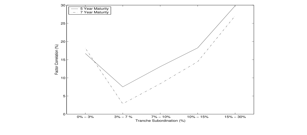
Plot of the average implied correlation estimates for different subordination levels for CDX for 5 and 7-year maturities. The implied correlation estimates are obtained using a static model over the period of June 2006 to December 2007. Figure 2 Copy link
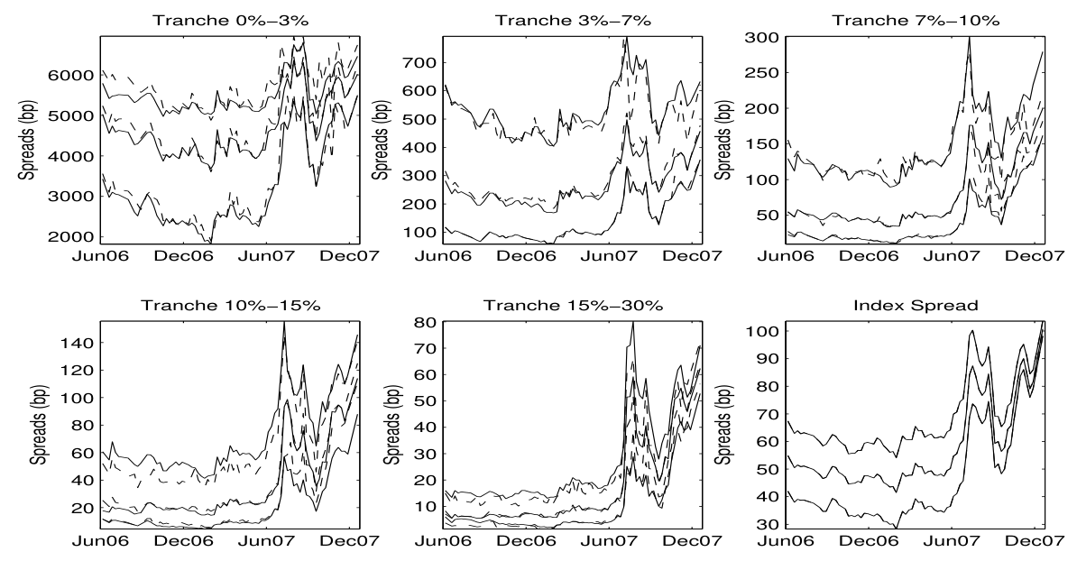
Plots of market and model implied tranche spreads for the CDX tranches for 5, 7 and 10-year maturities over the period of June 2006 to December 2007. A Gaussian mixture distribution was assumed for the idiosyncratic distribution H with one autoregressive lag in the common factor. Each panel shows the spreads for all maturities at a particular tranche subordination. The solid lines are the market quoted spreads. The dashed lines are the model implied spreads. Figure 3 Copy link
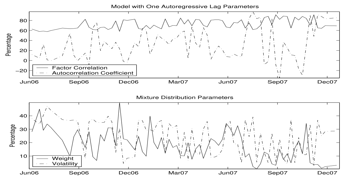
Parameter estimations using a Gaussian Mixture H distribution and one autoregressive lag in the common factor. The data calibrated to is the CDX tranches for 5, 7 and 10-year maturities over the period of June 2006 to December 2007. The top panel shows the parameters independent of the choice of idiosyncratic distribution H, so the factor correlation, ρ, and the common factor autoregressive coefficient, φ. The bottom panel shows a time-series of the parameters specific to a Gaussian mixture model as choice for H. These are the weight between the two Gaussian distributions, λ, and the volatility of the second distribution, σm.