

A new market is emerging in securitisations backed by the loans of Multilateral Development Banks (MDBs). Five MDBs have completed securitisations in recent years. The volume of transactions remains small relative to established securitisation asset classes (the pool loans of deals completed have notional value around $7.5 billion). But the scope for more transactions is considerable and several MDBs have planned issuance programs stretching into the future. Two initiatives by the World Bank Group (WBG) and the African Development Bank (AfDB) envisage creating multi-issuer platforms to which several MDBs could contribute loans.
Executive Summary
A new market is emerging in securitisations backed by the loans of Multilateral Development Banks (MDBs). Five MDBs have completed securitisations in recent years. The volume of transactions remains small relative to established securitisation asset classes (the pool loans of deals completed have notional value around $7.5 billion). But the scope for more transactions is considerable and several MDBs have planned issuance programs stretching into the future. Two initiatives by the World Bank Group (WBG) and the African Development Bank (AfDB) envisage creating multi-issuer platforms to which several MDBs could contribute loans.
Agency ratings strongly influence the economics of MDB securitisation. They do this through two separate channels:
1. The agencies’ supranational rating methodologies affect the benefits that MDBs obtain from reductions in risk (as measured by the agencies’ capital adequacy metrics)
2. How the agencies rate securitisations affect the cost to MDBs of obtaining tranched credit protection when those tranches are rated (for example in a true-sale Collateralised Loan Obligation (CLO)) or the capital cost to the MDB of retained securitisation tranches (either in a CLO or in a synthetic securitisation).
Since MDB loans constitute a new asset class for the structured finance departments of the major rating agencies, one may ask whether the assumptions that the agencies adopt in performing their analysis are truly appropriate for the risks involved? The credit quality of MDB loans has recently been investigated by a series of statistical reports (see Risk Control (2024) and (2025)) and studies issued by a consortium set up by MDBs to collect and investigate the performance of loans issued by its members (see Global Emerging Markets (GEMs) Risk Database (2025)). Individual MDBs have also issued analyses of the historical credit performance of their own loans (see IFC (2024)).
This study investigates the assumptions about MDB loans made by the rating agencies and shows the extent to which they are constraining the development of securitisation issuance by MDBs. We start by explaining how the agencies rate supranationals and tranches of securitisations they issue from their own balance sheet. It then presents a detailed but straightforward and realistic calculation using the methodologies of the agency that employs the most transparent approaches in both areas, Standard & Poor’s.
The calculation demonstrates very clearly the extent to which the economics of MDB securitisation are affected by the rating agency view of the underlying loan credit risk. Specifically, we consider a CLO of Non-Sovereign Obligor (NSO) loans with a stylised pool and structure comparable to those recently issued by the International Finance Corporation (IFC).
We devise a structure containing a series of tranches from most senior (AAA-rated) down to low rating grades and finally an unrated junior tranche. In each case, the tranches are devised to be the maximum possible thickness for the grade in question minus a buffer. Market spreads corresponding to different rating grades are assigned to the tranches to ensure that pricing is consistent with the way investors price risk. At the bottom of the capital stack, the Internal Rate of Return (IRR) for the junior tranche is estimated using Monte Carlo simulations of the underlying pool loans and the payments to different tranches implied by the structure.
The structuring analysis just described is performed, first, under the assumptions about pool credit performance employed by Standard & Poor’s and, second, under assumptions that we regard as more consistent with empirical evidence on MDB loans. We show that adopting Probabilities of Default (PDs) and mean Loss Given Default (LGD) rates consistent with three decades of historical performance, the IRR on the junior tranche is dramatically higher than that obtained when the structuring is determined by the current rating agency treatment.
The paper as a whole is broader than this numerical exercise, since it also examines how the agencies' supranational rating methodologies recognise risk transfer. The numerical exercise itself identifies the capital structure that the Standard & Poor's models support under a given set of assumptions. This should be distinguished from the structure and credit enhancement an agency would ultimately be prepared to rate, the prices at which investors would buy each tranche, the resulting economics for the MDB, and whether those economics would be repeatable across different market conditions. Section 4.1 sets out these distinctions.
© Copyright Risk Control Limited 2026
We conclude that the assumptions the agencies adopt on MDB loans, as exemplified by the Standard & Poor’s assumptions we apply, are extremely conservative and that this substantially affects the efficiency of MDB securitisation.
This conservatism should be understood in context. MDB loans are a new asset class for the structured finance departments of the agencies. Agency structured finance methodologies are designed for the high-volume asset classes that make up the bulk of their business. For asset classes outside that set, for which there is little deal volume, generic and conservative assumptions are inevitable and there is nothing improper in this. The agencies will only consider developing tailored approaches if an asset class becomes economically significant and a case is made on the basis of statistical evidence. We do not claim that this study by itself provides all the evidence the agencies would require. Our primary aim is rather to show senior MDB managers how material it is for the viability of risk transfers that agency methodologies appropriately reflect the nature of MDB loan risk and, hence, why an effort by MDBs to make that case is worthwhile.
As regards LGD rates for the higher rated tranches, the agency on which we focus here (which has the most transparent methodology of the three global agencies), Standard & Poor’s, assumes LGDs for corporate exposures in Group C countries (which includes most countries represented in MDB portfolios) in excess of 81.52% (see Table A4.2 in Appendix 4). This LGD assumed by the agency is a stressed version of a base LGD of 65.8%. GEMs data suggests the base LGD is 27.1%. The mean LGDs assumed by Fitch when evaluating highly rated tranches is even higher while that of Moody’s is somewhat less conservative.
In comparing these figures (particularly for Standard & Poor’s and Fitch), it is important to distinguish between
(i) historical average recoveries on defaulted loans, such as those reported by GEMs, (ii) recoveries conditional on default in stressed periods and, (iii) the recovery assumed when sizing a tranche to withstand a AAA or other high rating stress. The agency LGDs cited above (at least for Standard & Poor’s and Fitch) are stressed values of the third kind.
Stressing LGDs in this way is a simple device for reflecting the tendency of recoveries to be low when defaults are common, in models that do not represent the correlation between PDs and LGDs directly. However, the degree of PD-LGD correlation needed to generate stresses of this magnitude is very great. In our alternative case, we therefore do not apply the GEMs historical average to highly rated tranches directly but scale it using the stress pattern embedded in Standard & Poor’s own assumptions (see Appendix 4).
It is harder to observe directly how the agencies approach the mapping exercises that they employ to convert MDB internal ratings into the usual AAA to CC alpha-numeric scale. This mapping determines how conservative or otherwise the agency is as regards PDs. It is through this mapping, rather than through the published structured finance criteria, that the benefits of MDBs’ preferred creditor status and of the reduced transfer risk on MDB loans would be reflected. The process is not transparent, even to the originating MDB.
In the calculations presented in this study, we presume that the agencies are influenced by the sovereign rating cap that they typically apply and, hence, assign a rating to corporate loans on average 1 notch below the corresponding sovereign rating. Analysis we have performed on public data from IFC suggests that MDB’s historical default rates are consistent with a 1-notch-above-sovereign grading of corporate loans.
These are modelling assumptions. In the absence of internal MDB rating data, benchmarking against sovereign ratings is the only way of calibrating a pool using public information alone. It is also, in our view, the most obvious check an agency would apply to the appropriateness of an MDB’s mapping of its internal ratings. For loans to borrowers in Emerging Market and Developing Economy (EMDEs), the sovereign rating ceiling is a key consideration, unlike in the European or US CLO transactions for which agency mapping practice has largely been developed.
Under the assumptions about LGDs and PDs just described, we show that a CLO with the tranching devised in Section 4 receives an IRR spread over SOFR of 11% compared to a spread close to zero under the agency assumptions. On the Benefit to Cost (BTC) ratio that several MDBs now employ to measure the efficiency of risk transfers, the reasonable PD and LGD assumptions we employ imply a BTC ratio of 1.4 compared to a value of 0.7 under the agency assumptions. Section 4 shows the effects of the PD and LGD assumptions separately as well as in combination.
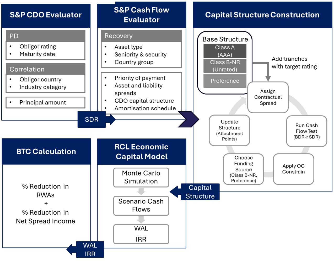
Figure ES1.1 shows graphically the numerical calculation implemented in this report. For a given pool, we employ CDO Evaluator and Cashflow Evaluator to construct the structure, assigning contractual spreads for
© Copyright Risk Control Limited 2026 tranches (based on ratings) so for each tranche the cash flows are consistent with the rating agency assessments. Having designed the structure, we estimate the Weighted Average Life (WAL) and Internal Rates of Return (IRRs) to estimate the Benefit to Cost (BTC) ratio for the deal.
To conclude, MDB securitisation has an important role to play in introducing new developed market investors to taking exposure, matching their risk appetite, to EMDE debt. MDBs and investors in the early deals can serve as pioneers and the ‘demonstration effects’ of these transactions (as described in Risk Control (2026a)) could ultimately lead to non-MDB issuance by EMDE banks and asset managers. The case made in this paper is that investors and the rating agencies, as gatekeepers to the new market, should be careful to base decisions on evidence and data and not on generic conservative criteria. The mobilisation and demonstration benefits of MDB securitisation are important for the development impact of MDBs, but they are analytically separate from the credit assessments the agencies perform, and we do not suggest that they should influence rating outcomes.
Figure ES1.1: Analytical Workflow
What would be necessary for the ratings agencies to change their methodologies. Rating agencies are commercial that organisations have both pecuniary and reputational motivations in deciding whether to make methodology changes:
(i) If agencies think the market will be large enough for them to make money, they will be more willing to consider modifications in their approaches. Otherwise, they will stick to standard approaches.
(ii) Agencies will only be willing to make changes if they are presented with evidence. This is appropriate: methodologies should change only to the extent that a proper case is made on the basis of statistical evidence on the credit performance of the loans.
To bring about changes in agency methodologies, therefore, MDBs need to generate sufficient deal volume to make it commercially interesting to the agencies and they must also provide convincing evidence. Evidence does not simply mean raw data but also apposite analysis. The issues on which agencies will want evidence are:
(a) Is there lower transfer risk in MDB loans than public bonds or loans from commercial banks justifying the idea that MDB loans be rated in a mapping exercise as higher than the corresponding sovereign
(b) How do LGDs behave in stressed EMDE credit market conditions. The current extreme LGDs employed by the agencies for NSO loans in EMDE countries are justified by the notions that recoveries are low
© Copyright Risk Control Limited 2026 when defaults are common. This argument can be taken to unrealistic extremes when no good evidence is available.
The data of the MDB undertaking a transaction will be central to any mapping exercise. The pooled GEMs statistics provide valuable market-level evidence but conceal significant variation in credit performance across MDBs, and a prudent agency will wish to understand the history of the specific originator. MDBs with long runs of data, such as IFC or AfDB, should be able to support mappings on which they and the agencies can rely. MDBs with shorter histories will have to accept the additional conservatism the agencies will naturally and correctly require until their records lengthen. In all cases, progress is most likely to come through dialogue with the agencies, transparency and systematic provision of data.
The target audiences for this study are, first, senior MDB and DFI management and shareholders, for whom the importance of rating agency methodologies for the development of MDB-loan securitisation markets may not be fully apparent and, second, the rating agencies themselves which, we hope, will be open to reconsidering aspects of their approaches if appropriate evidence is provided. Correctly calibrating risk and rating models for EMDE risk is an initial step in opening these debt markets to a broader cross-section of developed country investors.
© Copyright Risk Control Limited 2026
1. Introduction
Multilateral Development Banks (MDBs) face growing pressure to expand development lending while maintaining strong capital adequacy and high credit ratings[1]. Securitisation and other credit risk transfer techniques can, in principle, help MDBs recycle balance sheet capacity by transferring part of the credit risk on existing loan portfolios to investors or guarantors.[2]
MDBs undertake such transactions to manage their balance sheets consistently with their risk appetite, capital policies and long-term financial sustainability, and agency criteria are one important external reference point within that framework. Using risk transfer to strengthen capital ratios and thereby support ratings is analogous to a commercial bank transferring risk to meet its regulatory capital requirements.
MDBs’ ability to use securitisation as a balance sheet management tool is strongly influenced by the methodologies applied by the major credit rating agencies. These methodologies differ in the extent to which they recognise MDB risk transfer and in the capital adequacy measures they emphasise.
Standard & Poor’s applies a relatively risk-sensitive framework and more directly recognises the potential capital benefit of securitisation through its effect on risk-weighted assets (RWAs) and the risk-adjusted capital (RAC) ratio. Fitch also applies a risk-weighted capital framework, with particular emphasis on the Fitch usable capital to risk-weighted assets (FRA) ratio.
Moody’s proposed revisions to its supranational methodology, published for comment on 27th February 2026, can be summarised as moving the capital adequacy assessment away from a leverage-based measure towards a more risk-sensitive equity-to-risk-weighted-assets framework. This shift is closer in concept to Fitch’s approach and could increase the relevance of securitisation and other forms of risk transfer in Moody’s assessment of MDB balance sheet optimisation.
The analysis in this report proceeds in two stages.
(i) The relevant credit rating agency frameworks are summarised. In this, two aspects of the agency methodologies are particularly relevant: (a) the ways in which they allow for securitisation when they rate the MDBs themselves and (b) how the agencies approach rating securitisations that have MDB loans as underlying assets. (b) has a strong effect on the terms at which the MDBs are able to place the securitisation notes in funded transactions or the Risk Weights they must employ for retained tranches in the case of synthetic transactions.
(ii) The Standard & Poor’s CLO/CDO-style approaches are applied to a stylised demonstration portfolio, using the agencies’ published assumptions and model logic as closely as possible. The transaction we employ is the same stylised securitisation deal analysed in Risk Control (2026b), a profile of recent Collateralised Loan Obligations (CLOs) issued by the International Finance Corporation (IFC).
We focus on two aspects of the credit performance of MDB loans, their Probability of Default (PDs) and their mean Loss Given Default (LGD) rates. When rating a bank CLO using a Structured Finance methodology, agencies typically map the bank’s internal rating grades to the agencies’ own common alpha-numeric scale from (AAA to CC). The mapping process involves examination of the bank’s historical default experience and the scoring approach employed.
The sovereign ratings are a key benchmark because in rating any Non-Sovereign Obligor (NSO), rating agencies tend to apply a so-called ‘sovereign rating cap’. This approach reflects the notion that if a sovereign defaults, it will close the foreign exchange market, preventing local entities with external loans or bond issues from servicing their debt. MDBs may argue that their special access to sovereigns means that their NSO borrowers will be able to access foreign exchange even when the sovereign is in default, mitigating or eliminating ‘transfer risk’ for their NSO loans.
In our exercise, to deduce PDs, we benchmark NSO borrower ratings against those of the corresponding sovereigns, assuming they are given some number of notches above or below the SO ratings. The publicly available historical loss rates on IFC loans data of IFC suggest that the loans should be rated 1 notch above the corresponding SO ratings[3]. On the other hand, we hypothesise that the rating agencies, when performing mapping between internal MDB ratings and their own rating scale take the mapped ratings to be on average 1 notch below the SO ratings. These are modelling assumptions. In the absence of MDB internal rating data, benchmarking against sovereign ratings is the only way of calibrating a pool using public information alone. It is also, in our view, the most obvious check an agency would apply to the mapping of an MDB’s internal ratings, given the importance of the sovereign rating ceiling for NSO loans in the EMDE countries in which MDBs lend[4].
In examining the LGDs employed by the rating agencies in applying Structured Finance methodologies to securitisations, we contrast what are exceedingly conservative calibrations by the agencies to the LGDs reported by the GEMs data consortium. The latter are in the region of 30% while Standard & Poor’s, for example assumes around 60% as a base and a stressed value greater than 80% for rating AAA tranches.
The study is organised as follows. Section 2 describes how securitisations enter the agencies’ assessment of MDBs. Section 3 explains the approaches that the three agencies employ in evaluating the type of securitisation that MDBs issue. Section 4 sets out a detailed analysis of a representative MDB CLO transaction of the kind recently issued by the IFC.
2. MDB Ratings and Securitisation
2.1 Standard & Poor’s
Under Standard & Poor’s supranational methodology, securitisation affects an MDB primarily through the capital adequacy assessment. The key metric is the RAC ratio, defined as Total Adjusted Capital (TAC) divided by Risk Weighted Assets (RWAs). Securitisation is therefore relevant where it changes the MDB’s retained riskweighted exposure.
Standard & Poor’s (2025) identifies three broad forms of risk transfer: (i) synthetic risk transfer, (ii) securitisation of risk exposure, and (iii) risk transfer through financial guarantees [5]. Once Standard & Poor’s has concluded that the form of risk transfer is effective and can give rise to capital relief, it assesses the magnitude of the risk transfer by estimating the losses on the underlying portfolio.
Standard & Poor’s may use one of the following analytical approaches to estimate portfolio losses or establish the credit inputs required for the analysis:
1. A RACF-based adjusted total loss approach, under which portfolio losses are estimated and adjusted for economic strength, concentration, and diversification effects [6].
2. The CLO / corporate CDO criteria, which provide a more developed modelling framework for deriving tranche-level ratings through portfolio stress analysis and cash flow tests.
3. The CDO mapping criteria, where third-party internal scores are first translated into Standard & Poor’s global rating scale.
Standard & Poor’s then considers the resulting loss estimates in the context of the risk-transfer structure, including the attachment and detachment points, subordination and credit enhancement available to each tranche [7]. This analysis is used to infer a rating estimate for each tranche, which in turn determines the applicable risk weight.
For retained risk, Standard & Poor’s states that the equity tranche is typically assigned a 1250% risk weight. Retained mezzanine and senior tranches are instead assigned rating-based risk weights, as summarised in Table 2.1.
If a transferred tranche is fully funded and collateral is segregated in a way that removes counterparty uncertainty, Standard & Poor’s can treat the corresponding risk as effectively removed. If the protection depends on the offtaker’s promise to pay, the residual exposure instead depends on the credit quality of the offtaker or guarantor. Guaranteed tranches can receive risk substitution treatment if the guarantee meets the standard conditions of timeliness, irrevocability, and unconditionality.

Show as data
| Securitisation rating | AAA | AA | A | BBB | BB | B | CCC-C | Not rated or deducted from regulatory capital* |
|---|---|---|---|---|---|---|---|---|
| Risk weights (%) | 20 | 30 | 50 | 100 | 626 | 1,050 | 1,250 | 1,250 |
Note: * This risk weight applies when Standard & Poor’s have received a breakdown by rating or regulatory risk weight, but some exposures are unrated or deducted from regulatory capital. When breakdown by rating or regulatory risk weight for any of the exposure is not available, paragraph 96-98 in Standard & Poor’s (2024) applies.
2.2 Fitch
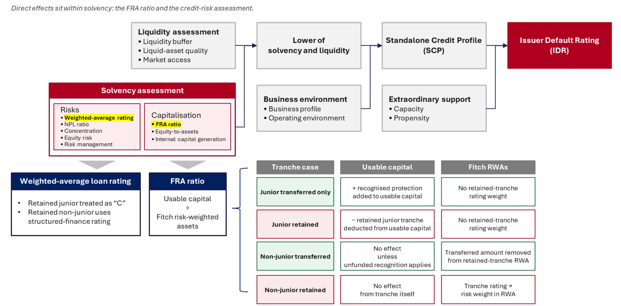
Under Fitch’s supranational methodology (see Fitch (2024)), securitisation matters primarily through its effect on the MDB’s solvency assessment, whose main capital anchor is the FRA ratio. Fitch explicitly recognises two forms of risk transfer:
1. First-Loss Piece (FLP) guarantees and
2. Synthetic securitisations.
An FLP guarantee is treated as additional loss-absorbing support and may be added to usable capital when calculating the FRA ratio. The recognised amount is reduced according to the credit quality of the guarantor. A similar treatment applies to a synthetic securitisation where only the most junior tranche is transferred: the transferred first-loss protection is recognised in the numerator of the FRA ratio as an addition to usable capital.
Where tranches other than the junior tranche are transferred, Fitch instead applies a retained-tranche approach. Any junior tranche retained by the MDB is deducted from usable capital, net of specific provisions relating to the securitised portfolio. The retained junior tranche therefore reduces the numerator of the FRA ratio and is treated as having a ‘C’ rating when Fitch calculates the weightedaverage rating of the loan portfolio.
Any retained mezzanine or senior tranche is assessed under Fitch’s Global Structured Finance Rating Criteria (Fitch (2025)). The resulting tranche rating determines the risk weight applied to that retained tranche in the denominator of the FRA ratio. The rating is also used when calculating the weightedaverage rating of the MDB’s loan book.
Transferred mezzanine or senior tranches do not form part of the MDB’s retained risk-weighted tranche exposure, although unfunded transfers remain subject to the credit quality of the protection provider. Funded transferred tranches are not discounted where the funds are placed within the MDB.

Show as data
| Loans, guarantees, treasuries, bond funds | AAA | AA | A | BBB | BB/B | CCC and below | equity participations |
|---|---|---|---|---|---|---|---|
| Risk weights | 0 | 20 | 30 | 50 | 100 | 150 | 250 |
Note: All values are expressed as percentages.
2.3 Moody’s
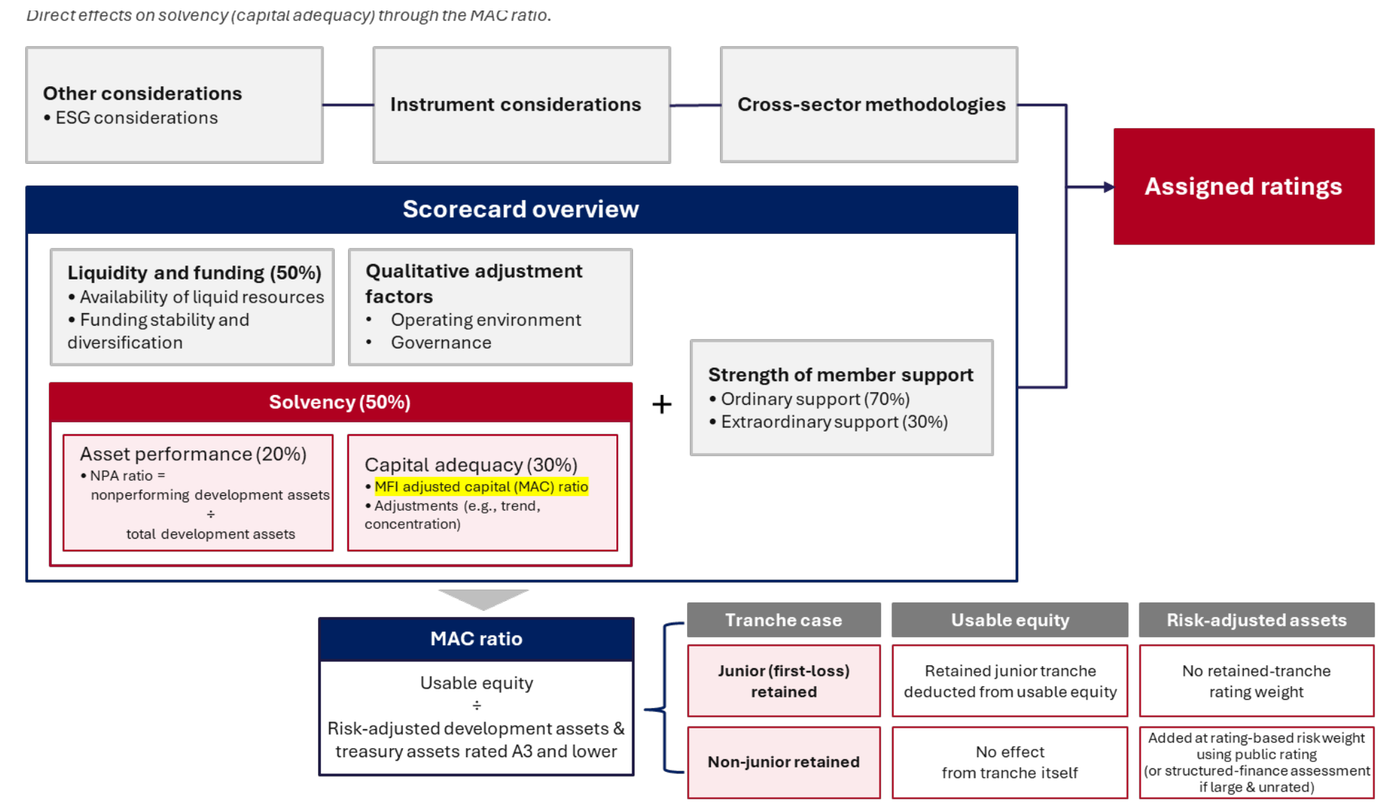
Under Moody’s revised methodology for multilateral financial institutions (see Moody’s (2026)), securitisation affects the issuer rating principally through the Solvency factor, which has a 50% weight in the scorecard for MDBs and Multilateral Development Finance Institutions (MDFIs). The Solvency factor comprises
1. Capital adequacy (with a 30% weight), and
2. Asset performance (with a 20% weight).
© Copyright Risk Control Limited 2026
Capital Adequacy is measured by the MFI Adjusted Capital ratio, calculated as Useable Equity divided by Risk- Adjusted Development Assets and Treasury Assets Rated A3 and Lower.
Risk-Adjusted Development Assets are calculated after deducting specific provisions and applying rating-based risk weights, taking account of Preferred Creditor Treatment (PCT) and eligible credit enhancements. Moody’s, therefore, recognises securitisation directly in the calculation of the MFI’s retained risk exposure.
Moody’s states that an MFI will typically retain the most junior, first-loss tranche and transfer mezzanine or senior tranches, or both, to external investors through either a true-sale or synthetic structure.
Where public ratings are available for some or all of the securitisation tranches, Moody’s uses those ratings as inputs to its risk-adjusted capital calculation. The amount of any retained first-loss tranche, net of specific provisions relating to the securitised portfolio, is deducted from useable equity.
For large unrated securitisations, Moody’s applies structured-finance principles to assess the credit quality of the tranches retained by the MFI.
Moody’s may also adjust the Capital Adequacy assessment for the expected trend in the MAC ratio and for portfolio concentration. Accordingly, the ultimate rating benefit may depend not only on the immediate reduction in retained risk, but also on the size and concentration of the remaining exposures and on how any released balance-sheet capacity is expected to be used.
© Copyright Risk Control Limited 2026
© Copyright Risk Control Limited 2026
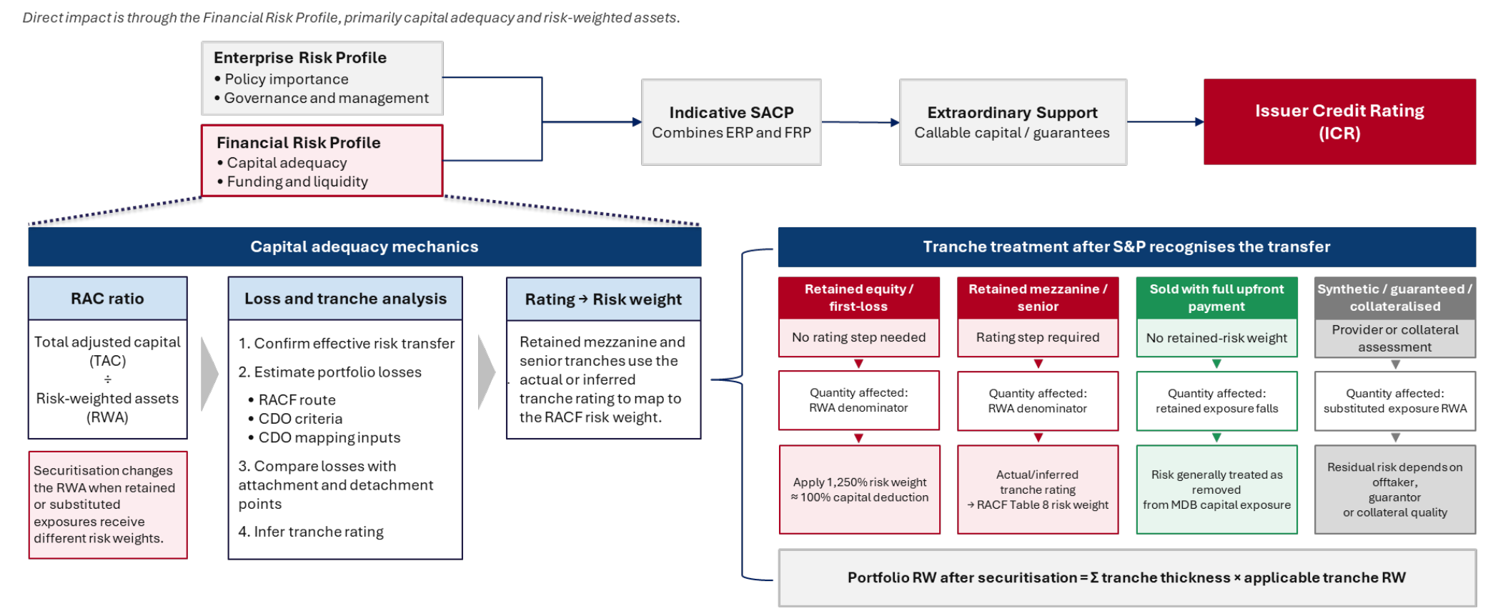
Note: Retained equity is typically assigned a 1,250% risk weight. For high-risk exposures, Standard & Poor’s may cap the applicable risk weight at the reciprocal of the MDB’s RAC ratio, so that allocated capital does not exceed the exposure amount.
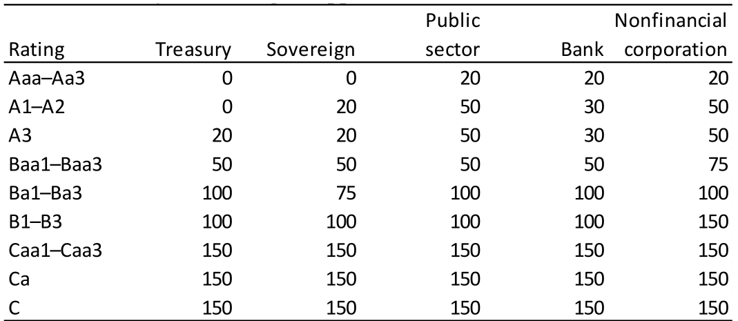
Show as data
| Rating | Treasury | Sovereign | Public sector | Bank | Nonfinancial corporation |
|---|---|---|---|---|---|
| Aaa–Aa3 | 0 | 0 | 20 | 20 | 20 |
| A1–A2 | 0 | 20 | 50 | 30 | 50 |
| A3 | 20 | 20 | 50 | 30 | 50 |
| Baa1–Baa3 | 50 | 50 | 50 | 50 | 75 |
| Ba1–Ba3 | 100 | 75 | 100 | 100 | 100 |
| B1–B3 | 100 | 100 | 100 | 100 | 150 |
| Caa1–Caa3 | 150 | 150 | 150 | 150 | 150 |
| Ca | 150 | 150 | 150 | 150 | 150 |
| C | 150 | 150 | 150 | 150 | 150 |
Note: All values are expressed as percentages.
3. How the Agencies Rate Securitisations
3.1 Standard & Poor’s
Standard & Poor’s applies a two-step framework to derive tranche-level ratings. First, it calculates the loss distribution of the underlying portfolio using a stochastic model. Second, it performs a cash-flow analysis of the transaction structure.
Specifically, Standard & Poor’s compares the Scenario Default Rate (SDR) produced by the credit model with the Break-Even Default Rate (BDR) implied by the structure. A tranche can be assigned a given rating only where the SDR associated with that rating level is at or below the BDR.
The credit analysis is performed using the CDO Evaluator, a Monte Carlo simulation model that generates a distribution of potential portfolio default rates. The SDR is represented as a percentile outcome of the simulated default distribution consistent with the target rating level [8]. This SDR reflects the level of portfolio defaults that could occur under severe but plausible stress conditions and forms the basis for the credit risk assessment.
We focus on the three key components driving the credit risk analysis, namely (i) the PD assumption, (ii) asset recovery assumptions, and (iii) correlation assumptions.
• PD The assigned rating based on the hierarchy of available rating information (Table A1. 1) is mapped to a PD using Standard & Poor’s calibrated default tables, which depend on both the rating category and the tenor of the instrument. Table 3.1 presents PDs for selected tenors (1, 5, and 10 years) for brevity [9].
• LGD Standard & Poor’s (2026b) determine asset recovery assumptions according to the following priority [10]:
1. Asset-specific recovery indicator: where a recovery indicator is available for the specific asset, this is used directly [11].
2. Pari passu recovery indicator: where the specific asset does not have its own recovery indicator, but a pari passu instrument has one, the pari passu recovery indicator may be used as a proxy.
3. No recovery indicator: where neither an asset-specific nor pari passu recovery indicator is available, the asset is assigned a recovery assumption based on its corporate asset type, seniority, security, and country grouping. This third approach appears to be more conservative.
It should be noted that Standard & Poor’s corporate recovery rating framework applies only to Group A and Group B jurisdictions. For Group C jurisdictions, Standard & Poor’s states that it does not assign recovery ratings, as recovery prospects cannot be determined with sufficient confidence.
Therefore, exposures from Group C countries would likely fall into the third recovery approach, which appears to apply lower and more conservative recovery assumptions. For CDOs, these assumptions are applied as fixed point estimates tiered by CDO liability rating. For synthetic CDOs, recovery rates are instead drawn from a beta distribution parameterised by a mean and standard deviation, reflecting the additional uncertainty around settlement values in credit derivative structures.
• Correlation The pairwise asset correlations are applied through a priority-based hierarchy, where more specific assumptions override the general mapping rules [12].
The hierarchy is applied as follows: specific pair-level overrides are considered first, followed by secondary override assumptions. Where no override is available, the correlation is determined based on the relationship between the two assets, including whether they share the same asset type, country, region, or are located in different regions.
For the cash-flow analysis, Standard & Poor’s reviews the transaction’s structural features, payment waterfall, level of enhancement and relevant covenants in order to determine the maximum level of defaults that the tranche can sustain. This maximum tolerable level of defaults is the BDR.
In doing so, it tests a range of scenarios based on key rating drivers, including the portfolio amortisation profile, default timing and patterns, recovery levels and timing, interest-rate stresses, foreign-exchange stresses where relevant, management fees, payment timing mismatch, and deferrable obligations. More details can be found in Standard & Poor’s (2020).
In addition to the standard CDO Evaluator analysis and the cash-flow analysis, Standard & Poor’s applies both supplemental tests and qualitative judgement when determining the final tranche rating.
The supplemental tests are quantitative checks designed to capture concentration, subordination, event risk and model risk that may not be fully reflected in the stochastic simulation. These include tests relating to the largest obligors, industry concentrations and the adequacy of subordination at the proposed rating level.
The qualitative judgement covers transaction-specific considerations that may require adjustments beyond the model outputs. These may include applying a cushion above the modelled SDR, taking a forward-looking view of changes in portfolio credit quality, and adjusting assumptions for recoveries, correlation, weighted-average spread or other portfolio characteristics.
For unusual portfolios, such as concentrated, skewed or bar-bell pools, Standard & Poor’s may also apply additional stresses or bias defaults towards particular parts of the portfolio.
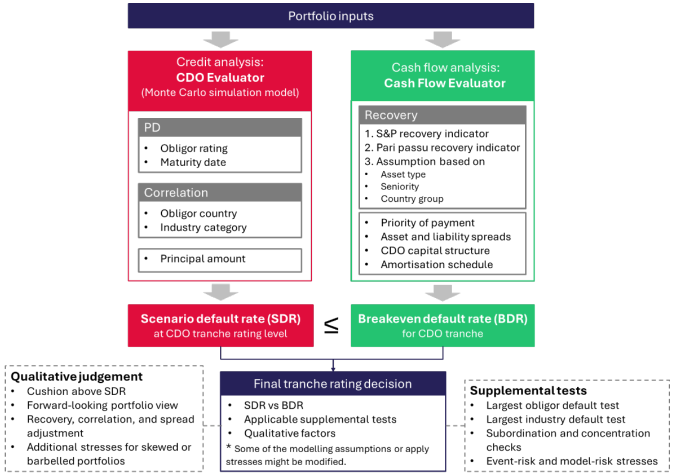
Note: Reproduced based on Standard & Poor’s (2019) Chart 1. Both CDO Evaluator and Cash Flow Evaluator are publicly accessible.
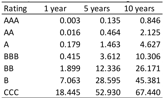
Show as data
| Rating | 1 year | 5 years | 10 years |
|---|---|---|---|
| AAA | 0.003 | 0.135 | 0.846 |
| AA | 0.016 | 0.464 | 2.125 |
| A | 0.179 | 1.463 | 4.627 |
| BBB | 0.415 | 3.612 | 10.306 |
| BB | 1.899 | 12.336 | 26.171 |
| B | 7.063 | 28.595 | 45.381 |
| CCC | 18.445 | 52.930 | 67.440 |
Note: All values are expressed as percentages.
3.2 Fitch
Fitch applies a two-stage framework to derive tranche-level ratings. First, it performs a credit analysis of the underlying portfolio. Second, it performs a cash-flow analysis of the transaction structure.
Fitch compares the Rating Default Rate (RDR) generated by its Portfolio Credit Model (PCM) with the BDR supported by the transaction structure. A tranche can support a given rating only where the BDR is at least equal to the corresponding RDR. The model-implied rating is the highest rating level at which the tranche passes the relevant stress scenarios.
The PCM is a Gaussian copula Monte Carlo model that simulates the joint default behaviour of the underlying assets. It maps the credit rating and maturity of each asset to a PD, applies recovery assumptions according to the security and jurisdiction of the exposure, and determines asset correlations based on industry, geography and obligor concentration.
We focus on the three key components driving Fitch’s portfolio credit analysis, namely: (i) PD assumptions, (ii) asset recovery assumptions and (iii) correlation assumptions.
• PD Fitch uses the issuer rating and the term of the asset as the main inputs to determine PD. The preferred input is the Fitch Issuer Default Rating (IDR) or Fitch Issuer Default Credit Opinion. Alternative input options are summarised in Table A2. 2 [13]. The PDs for selected tenors (1,5,10 years) are shown in Table 3.2 [14].
• LGD Fitch’s recovery framework is driven by two main factors: the jurisdiction of the obligor and the rating stress level being considered.
Fitch groups jurisdictions into three broad categories reflecting differences in creditor protection, insolvency regimes and expected recovery prospects. Group 1 broadly captures jurisdictions with stronger recovery environments, Group 2 intermediate recovery environments, and Group 3 weaker recovery environments [15].
Fitch assigns lower recovery assumptions in higher liability rating scenarios, such as ‘AAAsf’, and higher recovery assumptions in lower rating scenarios, such as ‘Bsf’. This reflects the methodology’s treatment of the pro-cyclical relationship between defaults and recoveries: in more severe stress scenarios, recoveries are assumed to be weaker.
Within that framework, Fitch applies two main routes:
1. Asset-specific recovery Where Fitch has assigned a Recovery Rating (RR1–RR6) or a specific recovery estimate to an asset, this information is used directly [16].
2. Standard recovery In the absence of asset-specific recovery information, Fitch applies standard recovery assumptions
17. These are based on the instrument type and capital structure position, using categories such as Strong recovery, Strong recovery MML, Senior secured bonds, Moderate recovery, and Weak recovery.
• Correlation The base correlation framework is shaped by two main dimensions: (i) the geographic relationship between obligors, and (ii) sector or industry commonality. The base framework is summarised in Table 3.3.
For the cash-flow analysis, Fitch reviews the transaction’s structural features, payment waterfall, level of credit enhancement and relevant covenants in order to determine whether the tranche can withstand the portfolio stress associated with each rating level.
The cash-flow model generates the BDR for each tranche, which is then compared with the rating default rate RDR derived from the PCM. A tranche can support a given rating only where the structure is able to withstand the corresponding stress scenario.
The Model-Implied Rating (MIR) is a key input to Fitch’s rating determination but does not mechanically determine the final tranche rating. Fitch’s rating committee may assign a rating that differs from the MIR after considering applicable rating caps, the size of the cushion between the tranche’s break-even default rate and the corresponding RDR hurdle, and the frequency with which the tranche passes the relevant cash-flow scenarios.
The committee may also assess whether the standard scenarios reflect its near-term expectations and may apply sensitivity analyses for concentration risk, specific issuers or sectors, asset prepayments, and changes in recovery expectations. Accordingly, the final tranche rating reflects the MIR together with additional quantitative analysis and transaction-specific qualitative judgement.
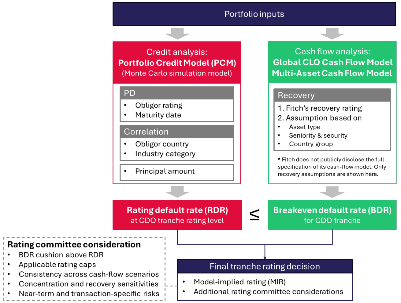
Note: Fitch’s PCM is publicly accessible. For the cash flow analysis, Fitch uses the Global CLO Cash Flow Model or, for selected non-US CLOs, the Multi-Asset Cash Flow Model. The cash flow model is not publicly available.
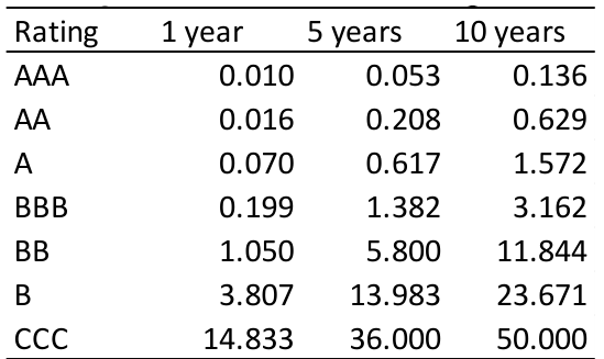
Show as data
| Rating | 1 year | 5 years | 10 years |
|---|---|---|---|
| AAA | 0.010 | 0.053 | 0.136 |
| AA | 0.016 | 0.208 | 0.629 |
| A | 0.070 | 0.617 | 1.572 |
| BBB | 0.199 | 1.382 | 3.162 |
| BB | 1.050 | 5.800 | 11.844 |
| B | 3.807 | 13.983 | 23.671 |
| CCC | 14.833 | 36.000 | 50.000 |
Note: All values are expressed as percentages.

Show as data
| Base level | Sector add-on | Industry add-on | |
|---|---|---|---|
| Same country | 10 (6 if US) | +2 | +20 |
| Same region, different countries | 6 | +2 | +20 |
| Different regions | 4 | +2 | +20 |
| Banking and finance assets | As above | +14 | +8 |
Note: All values are expressed as percentages.
3.3 Moody’s
Moody’s uses the CDOROM model to simulate portfolio defaults, recoveries and losses. The simulated portfolio losses are allocated through the transaction’s capital structure to calculate the Expected Loss (EL) of each tranche. The tranche EL is then compared with Moody’s idealised expected-loss benchmarks, taking account of the tranche’s weighted average life (WAL).
Unlike Standard & Poor’s and Fitch, Moody’s does not primarily compare a rating default rate with a breakeven default rate. Instead, the principal quantitative output is the tranche’s modelled EL.
The three principal drivers of the Moody’s credit analysis are: (i) rating and PD inputs, (ii) recovery and LGD assumptions and (iii) asset correlation assumptions.
• PD A base PD is inferred from the reference entity rating and the tenor of the exposure using Moody’s idealised default probability tables [18]. The rating framework applied is summarised in Table A3. 1.
After the initial rating input has been selected, Moody’s applies several further adjustments before finalising the modelled default probability used in CDOROM (Table A3. 2). Some of these are implemented by first adjusting the rating input, while others are expressed more directly as stresses to the default assumption.
• LGD The recovery assumption is driven primarily by the type of obligation and its position in the capital structure. Unless the transaction documentation specifies a fixed recovery value for credit events, Moody’s models stochastic recovery rates using beta distributions.
The mean and standard deviation of those distributions depend on the asset type, and the recovery processes are modelled as correlated (Table 3.4). Moody’s also states that exposures to different obligations within the same corporate family are modelled with 100% recovery correlation.
For synthetic transactions, Moody’s applies a further cheapest-to-deliver adjustment. Because credit events are usually defined at the reference-entity level rather than for a specific obligation, the protection seller may, within the eligible deliverable set, choose the cheapest-to-deliver asset when settling a defaulted name.
Moody’s therefore applies a 10% cheapest-to-deliver haircut to recovery assumptions for all assets. This means that the modelled recovery used in the tranche analysis is lower than the base recovery assumption shown above.
• Correlation Pairwise asset correlations depend primarily on three elements: (i) the reference entity’s credit rating,
(ii) its industry classification, and (iii) its country / region of domicile.
Moody’s divides the correlation structure into a base inter-industry component and an additional intraindustry component.
The inter-industry component captures the dependency between references regardless of sector or region, while the intra-industry component increases correlation where names share the same industry and, depending on the industry type, the same region.
Exposures to different obligations or entities within the same corporate family are modelled with 100% asset correlation.
Once reference-pool losses are simulated, they are passed through the tranche structure by Moody’s to derive the tranche’s modelled EL. The EL is defined as the average present-value loss across all simulated scenarios, and Moody’s applies a 99% confidence interval adjustment where relevant.
The modelled EL is then compared with Moody’s Idealized Expected Loss benchmarks, taking into account the tranche’s WAL. Moody’s uses a Wide Asymmetric Range, in which the lower bound of loss consistent with a given rating is the benchmark EL of the next higher rating category, while the upper bound for initial ratings is the benchmark EL of the rating category itself.
Moody’s frames the final tranche assessment primarily through an EL-benchmark comparison rather than an SDR/BDR or RDR/BDR test compared to the cases of Standard & Poor’s and Fitch. The final assigned rating may nevertheless differ from the model output because Moody’s supplements the quantitative analysis with qualitative considerations.
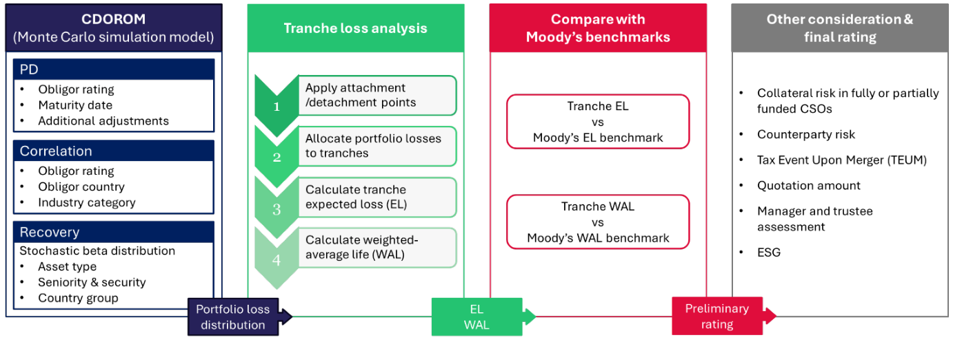
Note: Moody's CDOROM is not publicly available.

Show as data
| Asset type | Mean | Std dev. |
|---|---|---|
| Senior secured loans (first-lien only) | 40 | 25 |
| Senior secured loans (non-first-lien) and senior secured bonds | 55 | 30 |
| Senior unsecured bonds and senior unsecured loans | 65 | 30 |
| Subordinated bonds | 75 | 25 |
Note: All values are expressed as percentages. Std dev. denotes standard deviation.

Show as data
| Credit category | Inter-industry correlations | Weights |
|---|---|---|
| Investment-grade credits | 5, 10, 20 | 70, 20, 10 |
| Ba-rated credits | 3, 9, 12 | 70, 20, 10 |
| B-rated credits and below | 3, 7, 10 | 70, 20, 10 |
Note: All values are expressed as percentages.

Show as data
| Industry type | Same industry, different regions | Same industry, same region |
|---|---|---|
| Global | +12 | +0 |
| Semi-local | +6 | +6 |
| Local | +0 | +12 |
Note: All values are expressed as percentages. The designation of each industry is listed in Exhibit 8 of Moody’s (2024).
4. Agency Approaches and the Economics of Securitisation
4.1 Structuring exercise in summary
This section develops a structuring exercise designed to show how rating agency views on MDB loan portfolios affect the economics of securitisations the MDBs issue. The agencies, as gate-keepers of the securitisation market as far as investors are concerned strongly influence the pricing of different tranches. AAA-rated tranches in the CLO market trade within a relatively narrow range despite differences in underlying assets and the tranche structure of the deal.
If agencies are overly conservative in their evaluation of the PDs and LGDs of the underlying loans, this feeds through in relatively thin senior tranches (which are the cheapest to finance) and, thus, has an impact on the Internal Rate of Return (IRR) of the very lowest tranche in the structure, the equity tranche. One may examine this impact on the ‘economics of the deal’ by computing two quantities:
1. The IRR on the equity tranche (as just described)
2. The ratio of the percentage Risk Weighted Assets saved to the percentage spread income given up when a securitisation deal is done.
Demonstrating the magnitude of these effects requires that one devise a structure in which tranches are consistent with a set of ratings which in turn are aligned with the tranche pricing. Such an exercise is described in Figure 4.1. In this context, we focus on Standard & Poor’s ratings. Standard & Poor’s has the most transparent set of methodologies for corporate-debt-backed securitisations like CLOs. Both the way in which the agency estimates the pool default rate distribution and the tool it uses to model the cash flow waterfall are fully in the public domain. (Fitch is transparent about its approach to default rate distributions but not about cash flow waterfall modelling. Moody’s is the least transparent in its methodologies.)
The quantitative exercise should, therefore, be read as a Standard & Poor’s case study. We selected Standard & Poor’s because both of the tools it uses are publicly available, so that the exercise can be replicated. Fitch and
Moody’s employ different models and assumptions (see Section 3) and could reach different conclusions on the same pool. A cross-check against their approaches would be a natural extension but is harder to perform, since Fitch does not publish its cash flow model and Moody’s CDOROM model is not publicly available. The conclusions we draw relate to the effect of the selected Standard & Poor’s assumptions rather than to agency assumptions in general. An MDB contemplating a transaction would, in any case, test the structure directly with the structured finance teams of the agencies.
The numerical exercise answers a specific question: what capital structure the Standard & Poor's models support under the chosen assumptions. Using stylised tranche spreads, it also estimates the resulting economics for the MDB. It does not show what structure and credit enhancement an agency would ultimately be prepared to rate, since that also depends on the qualitative factors described in Section 4.4. Nor does it show the prices at which investors would actually buy each tranche, or whether the economics would hold up through different market conditions. Answering those questions would require engagement with the agencies and with investors on a live transaction.
In the subsections below, we apply the methodology depicted in Figure 4.1 to compute the default rate distribution and then to compute a price- and rating-consistent set of tranche attachment points.
The results depend on the assumptions employed. The pool is stylised, the rating of loans relative to the sovereign is a modelling assumption, the alternative recovery framework combines GEMs historical averages with a stress pattern taken from Standard & Poor's, and the tranche spreads are illustrative. We have not reconciled differences between the GEMs data and agency assumptions in default definitions, the treatment of restructurings and cures, or recovery timing, nor have we tested sensitivity to higher or more concentrated correlation. The numerical results should therefore be read as indicating the direction and approximate scale of the effect of agency assumptions on deal economics rather than as precise estimates for a particular transaction.
4.2 Hypothetical portfolio
A stylised transaction was constructed to replicate the principal publicly-disclosed features of the IFC EMSP 2025-1 transaction and its underlying collateral portfolio.
The transaction structure comprises two classes of secured notes: USD 320 million of senior Class A Notes, rated Aaa(sf) by Moody’s, and USD 130 million of unrated mezzanine Class B Notes. The Class B Notes are subordinated to the Class A Notes. The Preferred Shares, with a total value of USD 59.53 million, provide the residual financing required to fund the underlying asset pool, the reserve cash account and transaction-related expenses.
Accordingly, the interest reserve cash account is assumed to equal USD 7.63 million. This amount represents the difference between the total transaction funding of USD 509.53 million and the combined value of the USD 500 million underlying asset portfolio and USD 1.90 million of initial transaction costs.
The underlying portfolio has a total par value of USD 500 million and comprises 57 loans across 28 countries. The five largest country concentrations were based on publicly disclosed information relating to the EMSP 2025-1 portfolio. The remaining countries were selected from the universe of IFC member countries using income classification, sovereign credit rating and GDP criteria. The resulting portfolio has a weighted-average spread of 3.02% over SOFR and a WAL of approximately 3.3 years. The asset security was distributed between secured and unsecured loans as described in Appendix 4.
Two portfolio rating settings were considered. In the one-notch-above-sovereign case (labelled ‘Sov + 1’ in Table 4.2 to Table 4.4), which is consistent with the historical performance of IFC loans and is treated as the base case, each loan is assigned a rating one notch stronger than the corresponding sovereign rating. This produces an average portfolio rating of BB− and a weighted-average PD of 10.13%. In the one-notch-below-sovereign case (labelled ‘Sov - 1’), which reflects our hypothesis about the agency mapping, each loan is assigned a rating one notch weaker than the sovereign rating, producing an average portfolio rating of B and a weighted-average PD of 17.50%.
We follow the same correlation assumption as used in Standard & Poor’s (2019), the weighted-average pairwise correlation for the stylised portfolio is approximately 0.06 in both cases.
Two recovery frameworks were also considered for the cash flow analysis. The first follows Standard & Poor’s recovery methodology. The second recovery framework is based on GEMs data[19]. The detailed recovery assumptions are presented in Appendix 4[20].
4.3 Rating Agency LGD Treatment
The structuring exercise in this section applies Standard & Poor’s assumptions. To show how far this choice drives the results, we compare the Loss Given Default (LGD) rates that each of the three global rating agencies assigns to the stylised portfolio described in Sub-section 4.2. The comparison applies each agency’s standard assumptions for corporate loans. (Comparisons of PDs are harder to make. Each agency maps a bank’s internal ratings to its own scale. How this is done for a new asset class like MDB loans is opaque, although one may presume, as we do in earlier sections, that for an EMDE loan portfolio the agencies are influenced by the sovereign rating cap.)
As regards LGDs, the agencies differ in three aspects. First, Standard & Poor’s (2019) and Fitch (2023) apply deterministic LGDs that rise with the target tranche rating. This justified by the argument that losses on defaulted assets tend to be higher when defaults are widespread.[21] Moody’s (2024) instead simulates betadistributed LGDs assuming that the mean and standard deviation LGDs depend only on asset type and seniority. Moody’s assumes that LGDs are correlated across obligors through a single-factor Gaussian copula and does not adjust them when rating tranches of different ratings grades.
Second, Standard & Poor’s and Fitch differentiate LGDs by jurisdiction. Standard & Poor’s assigns countries without a jurisdiction ranking assessment to its lowest recovery group (Group C). Fitch places most emerging market countries, including Brazil, Mexico, Turkey, Egypt and India in its Group 3. Moody’s does not differentiate between loans from different regions arguing about recover rates that “North American and emerging market defaulted obligors have differed very little” (see Moody’s (2024)).
Third, each agency applies further adjustments that increase LGDs. Fitch increases the assumed LGD on the largest risk contributors by 25%. Standard & Poor’s apples flat, high LGDs in its supplemental largest-obligor and industry default tests. Moody’s applies a 10% cheapest-to-deliver haircut to recoveries in synthetic transactions.
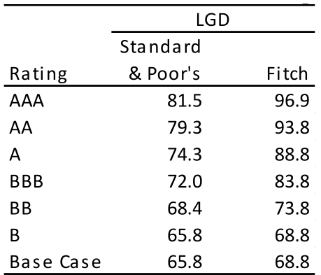
Table 4.1 reports the resulting Weighted Average LGDs. For Standard & Poor’s and Fitch, the table shows the LGD at each rating stress, with the base case corresponding to the lowest (‘B’) stress. For Moody’s, the mean LGD for the portfolio is 49.5%, with a standard deviation of 25% to 30% depending on the asset type.
Three conclusions follow. First, Fitch is the most conservative of the three agencies when evaluating highly rated tranches if the underlying loans are from EMDE countries. For the ‘AAA’ stress, it assumes an LGD of 96.9%, implying almost no recovery on defaulted loans. This compares to a Standard & Poor’s assumption of 81.5%. The gap narrows as the rating stress falls, and in the base case the two agencies’ assumptions differ by only three percentage points (68.8% and 65.8%).
Second, Moody’s mean LGD of 49.5% is 16 to 19 percentage points below the base-case assumptions of the other two rating agencies. This is a direct consequence of the agency’s policy of not penalising emerging market obligors. Because Moody’s does not tier LGDs by rating level, its mean LGD is not directly comparable with the stressed point estimates of Standard & Poor’s and Fitch. Moody’s models LGDs as correlated across obligors, and this may increase the severity of losses in the scenarios relevant to highly rated tranches above what the mean LGD alone would suggest.
Third, all three agencies assumed LGDs substantially above the 27.1% historical average reported by GEMs for MDB private-sector lending. Even Moody’s region-neutral mean is almost twice the GEMs figure, while Standard & Poor’s and Fitch base-case LGDs are around two and a half times higher.
The comparison also bears on the interpretation of the results in Sub-section 4.5 and 4.6. Had the structuring exercise used Fitch rather than Standard & Poor’s LGDs, the senior tranches would have been thinner still and the economics of the transaction weaker
Show as data
| LGD | ||
|---|---|---|
| Rating | Standard & Poor's | Fitch |
| AAA | 81.5 | 96.9 |
| AA | 79.3 | 93.8 |
| A | 74.3 | 88.8 |
| BBB | 72.0 | 83.8 |
| BB | 68.4 | 73.8 |
| B | 65.8 | 68.8 |
| Base Case | 65.8 | 68.8 |
4.4 CDO Evaluator
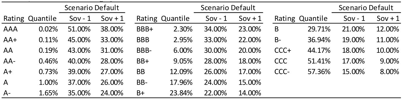
The analysis first uses Standard & Poor’s CDO Evaluator to estimate the SDR associated with different trancherating stresses. The model simulates a distribution of possible portfolio default rates and uses this distribution to calculate the gross level of defaults that a tranche at each rating level is expected to withstand.
The detailed amortisation profile of the portfolio is not modelled within the CDO Evaluator. The portfolio is therefore represented as a bullet portfolio with a maturity of 3.3 years, equal to the WAL of the underlying loans. This provides a single maturity assumption that is broadly consistent with the average period over which the portfolio remains exposed to credit risk.
The CDO Evaluator is run separately for the one-notch-below-sovereign and one-notch-above-sovereign rating cases. The change in rating affects the default probability assigned to each loan and therefore the resulting scenario default rates. The portfolio composition, exposure sizes and correlation assumptions remain unchanged. The SDR results for the two rating cases are shown in Table 4.2.
At this stage, the analysis focuses on gross portfolio defaults. Recovery and LGD assumptions therefore do not affect the SDR results. The recovery assumptions are instead introduced in the cash flow model.
Show as data
| Scenario Default | Scenario Default | Scenario Default | |||||||||
|---|---|---|---|---|---|---|---|---|---|---|---|
| Rating | Quantile | Sov - 1 | Sov + 1 | Rating | Quantile | Sov - 1 | Sov + 1 | Rating | Quantile | Sov - 1 | Sov + 1 |
| AAA | 0.02% | 51.00% | 38.00% | BBB+ | 2.30% | 34.00% | 23.00% | B | 29.71% | 21.00% | 12.00% |
| AA+ | 0.11% | 45.00% | 33.00% | BBB | 2.95% | 33.00% | 22.00% | B- | 36.94% | 19.00% | 11.00% |
| AA | 0.19% | 43.00% | 31.00% | BBB- | 6.00% | 30.00% | 20.00% | CCC+ | 44.17% | 18.00% | 10.00% |
| AA- | 0.46% | 40.00% | 28.00% | BB+ | 9.05% | 28.00% | 18.00% | CCC | 51.41% | 17.00% | 9.00% |
| A+ | 0.73% | 39.00% | 27.00% | BB | 12.09% | 26.00% | 17.00% | CCC- | 57.36% | 15.00% | 8.00% |
| A | 1.00% | 37.00% | 26.00% | BB- | 17.96% | 24.00% | 15.00% | ||||
| A- | 1.65% | 35.00% | 24.00% | B+ | 23.84% | 22.00% | 14.00% |
4.5 Cash flow model and capital structure
The portfolio is then analysed using the cash flow model. The same portfolio composition, rating assumptions, correlations and spreads are retained, but the cash flow model additionally incorporates the portfolio amortisation profile, default timing, recovery rates, liability spreads, payment waterfall and coverage tests.
For each target tranche rating, the cash flow model calculates the BDR, defined as the maximum level of portfolio defaults that the tranche can withstand while continuing to meet its contractual interest and principal obligations. This is compared with the corresponding SDR generated by the CDO Evaluator. A tranche is considered to pass the quantitative test for a given rating where its BDR is equal to or greater than the SDR associated with that rating.
Passing this quantitative test is a necessary but not a sufficient condition for a tranche to achieve the target rating. The final rating also reflects supplemental tests and qualitative judgement described in Section 3, as well as transaction specific considerations such as legal enforceability, servicing, counterparty exposure, liquidity, hedging, asset eligibility, amendment rights, legal final maturity and, sovereign risk. The structures derived below are therefore best described as model-supported capital structures under the selected assumptions rather than as structures that would necessarily receive the stated ratings.
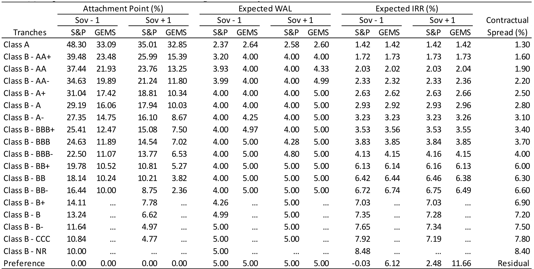
The cash flow analysis started with a simple base structure containing only Class A, Class B - NR, and the Preference tranche. This structure was used to identify the minimum attachment point required for the AAA tranche. After finding the minimum AAA attachment point, a 97% buffer was applied to the AAA tranche. The buffer ensures that the AAA tranche passes its test with a margin, i.e. that its BDR exceeds the AAA SDR rather than just equalling it, reflecting the cushion above the minimum model result that agencies typically look for. In standard structuring terms, each tranche is defined by its attachment point, shown in Table 4.3, and its detachment point, which equals the attachment point of the tranche immediately senior to it (100% for Class A). The protection each tranche enjoys can be measured by the excess of its BDR over the SDR for its rating and by that excess as a percentage cushion. We then gradually added lower-rated tranches below Class A to build out the full capital structure.
Several rules were followed when adding new tranches:
1. Tranche spreads were assigned in a stepwise manner The AAA spread was set at 1.3%, based on the IFC EMSP assumption. For each newly added tranche, the spread was increased by 30 bps relative to the previous tranche.
The BB tranche spread starts at 6.00%, after which each lower tranche again receives an additional 30 basis points. This produces a reasonable spread range when compared with observed market data [22]. The final spread assumptions are shown in Table 4.3 Contractual Spread column.
These spreads are illustrative rather than market-clearing levels. They are consistent with those reported in a reasonably authoritative industry source and applicable at the date of its publication, but not necessarily with current market conditions. The uniform 30 bp steps between rating grades are a modelling convenience; in practice, pricing rarely moves in uniform increments since different rating categories attract different investor groups. Investors in an MDB transaction would also price features beyond the rating, such as the novelty of the collateral, emerging market exposures, legal structure, pool disclosure, tranche size and absence of an established secondary market, which could add a new issue or liquidity premium, particularly on mezzanine tranches.
2. Tranche sizing was constrained by the OC test limits The thickness of each tranche could not exceed the limits implied by the relevant OC test. The minimum OC ratios were set at 1.48× for AAA-rated tranches, 1.06× for tranches rated from AA+ to BBB−, and 1.04× for all lower-rated tranches.
The OC ratio for a given tranche is the par value of the performing collateral divided by the par value of that tranche and all tranches senior to it. As in a conventional CLO, the OC tests operate through the priority of payments in the cash flow model; if a ratio falls below its required level, cash that would otherwise be paid to more junior tranches is diverted to redeem the senior notes until the test is restored. In the structuring exercise, we additionally required each tranche to satisfy its OC test at closing, which places an upper limit on the thickness of the tranche.
3. Lower-rated tranches were funded according to a defined hierarchy The lower-rated tranches were added using the available Class B - NR balance first. New tranches continued to be added as long as the unrated Class B balance was not exhausted. During this stage, the remaining unrated Class B tranche was assigned a spread equal to the spread of the lowest-rated tranche plus 60 bps.
Once the Class B - NR balance was exhausted, any additional lower-rated tranches were funded by reducing the thickness of the Preference tranche.
Following this process, we derived the final tranche thicknesses and attachment points for the full structure. The resulting capital structures are represented by the attachment-point columns in Table 4.3, which show the lower boundary of each tranche within the portfolio capital structure.
In three of the four scenarios, the iterative addition of rated tranches exhausts the available Class B-NR balance and begins to reduce the Preference tranche. The only exception is the one-notch-below-sovereign case under the Standard & Poor’s recovery assumptions, in which a residual Class B-NR tranche remains and the Preference tranche is not used to fund additional rated tranches.
Under both the one-notch-below-sovereign and one -notch-above-sovereign cases using Standard & Poor’s recovery assumptions, the structure can be extended down to a CCC-rated tranche. By contrast, under the GEMs recovery assumptions, the construction process terminates at BB− in both rating cases, because the addition of any further lower-rated tranche does not satisfy the quantitative requirement that the tranche BDR be at least equal to the corresponding SDR.
Based on each resulting capital structure, the tranche sizes, attachment points, and contractual spreads are then entered into our internal capital model to generate scenario-specific principal, interest, and total cash flows for each tranche. These cash flows reflect simulated defaults, recoveries, the transaction waterfall and the timing of distributions.
For each tranche, the WAL is calculated in each simulation as the principal-weighted average timing of principal repayments and is then averaged across all simulations.
For each simulation, the IRR is the annual rate at which the present value of the simulated interest and principal payments equals the tranche’s initial par. The expected IRR is subsequently calculated as the average of the simulated IRRs, and the expected spread is calculated as the difference between the expected IRR and SOFR.
The four scenarios in Table 4.3 form a two-by-two grid that allows the effects of the PD and LGD assumptions to be separated: (i) the one-notch-below-sovereign mapping with Standard & Poor’s recoveries corresponds to the agency treatment; (ii) the one-notch-below-sovereign mapping with GEMs-based recoveries changes only the LGD assumption; (iii) the one-notch-above-sovereign mapping with Standard & Poor’s recoveries changes only the PD assumption; and (iv) the one-notch-above-sovereign mapping with GEMs-based recoveries changes both. The expected IRR spread on the preference tranche is close to zero (-.03%) in case (i), 6.12% in case (ii), 2.48% in case (iii) and, 11.66% in case (iv). The recovery assumption therefore has the larger individual effect, but the two assumptions reinforce each other when changed together.
Show as data
| Attachment Point (%) | Expected WAL | Expected IRR (%) | ||||||||||||
|---|---|---|---|---|---|---|---|---|---|---|---|---|---|---|
| Sov - 1 | Sov + 1 | Sov - 1 | Sov + 1 | Sov - 1 | Sov + 1 | Contractual | ||||||||
| Tranches | S&P | GEMS | S&P | GEMS | S&P | GEMS | S&P | GEMS | S&P | GEMS | S&P | GEMS | Spread (%) | |
| Class A | 48.30 | 33.09 | 35.01 | 32.85 | 2.37 | 2.64 | 2.58 | 2.60 | 1.42 | 1.42 | 1.42 | 1.42 | 1.30 | |
| Class B - AA+ | 39.48 | 23.48 | 25.99 | 15.39 | 3.20 | 4.00 | 4.00 | 4.00 | 1.72 | 1.73 | 1.73 | 1.73 | 1.60 | |
| Class B - AA | 37.44 | 21.93 | 23.76 | 13.25 | 3.93 | 4.00 | 4.00 | 4.33 | 2.03 | 2.02 | 2.03 | 2.04 | 1.90 | |
| Class B - AA- | 34.63 | 19.89 | 21.24 | 11.80 | 3.99 | 4.00 | 4.00 | 4.99 | 2.33 | 2.32 | 2.33 | 2.36 | 2.20 | |
| Class B - A+ | 31.04 | 17.42 | 18.81 | 10.34 | 4.00 | 4.00 | 4.00 | 5.00 | 2.63 | 2.62 | 2.63 | 2.66 | 2.50 | |
| Class B - A | 29.19 | 16.06 | 17.94 | 10.03 | 4.00 | 4.00 | 4.00 | 5.00 | 2.93 | 2.92 | 2.93 | 2.96 | 2.80 | |
| Class B - A- | 27.35 | 14.75 | 16.10 | 8.67 | 4.00 | 4.25 | 4.00 | 5.00 | 3.23 | 3.23 | 3.23 | 3.26 | 3.10 | |
| Class B - BBB+ | 25.41 | 12.47 | 15.08 | 7.50 | 4.00 | 4.97 | 4.00 | 5.00 | 3.53 | 3.56 | 3.53 | 3.55 | 3.40 | |
| Class B - BBB | 24.63 | 11.89 | 14.54 | 7.02 | 4.00 | 5.00 | 4.28 | 5.00 | 3.83 | 3.85 | 3.84 | 3.85 | 3.70 | |
| Class B - BBB- | 22.50 | 11.07 | 13.77 | 6.53 | 4.00 | 5.00 | 4.80 | 5.00 | 4.13 | 4.15 | 4.16 | 4.15 | 4.00 | |
| Class B - BB+ | 19.78 | 10.52 | 10.81 | 5.27 | 4.00 | 5.00 | 5.00 | 5.00 | 6.13 | 6.14 | 6.16 | 6.13 | 6.00 | |
| Class B - BB | 18.14 | 10.24 | 10.21 | 3.82 | 4.00 | 5.00 | 5.00 | 5.00 | 6.42 | 6.44 | 6.46 | 6.38 | 6.30 | |
| Class B - BB- | 16.44 | 10.00 | 8.75 | 2.36 | 4.00 | 5.00 | 5.00 | 5.00 | 6.72 | 6.74 | 6.75 | 6.49 | 6.60 | |
| Class B - B+ | 14.11 | ... | 7.78 | ... | 4.26 | ... | 5.00 | ... | 7.03 | ... | 7.03 | ... | 6.90 | |
| Class B - B | 13.24 | ... | 6.62 | ... | 4.99 | ... | 5.00 | ... | 7.35 | ... | 7.28 | ... | 7.20 | |
| Class B - B- | 11.64 | ... | 4.97 | ... | 5.00 | ... | 5.00 | ... | 7.65 | ... | 7.34 | ... | 7.50 | |
| Class B - CCC | 10.84 | ... | 4.77 | ... | 5.00 | ... | 5.00 | ... | 7.92 | ... | 7.19 | ... | 7.80 | |
| Class B - NR | 10.00 | ... | ... | ... | 5.00 | ... | ... | ... | 8.48 | ... | ... | ... | 8.40 | |
| Preference | 0.00 | 0.00 | 0.00 | 0.00 | 5.00 | 5.00 | 5.00 | 5.00 | -0.03 | 6.12 | 2.48 | 11.66 | Residual |
Note: Attachment point is based on the target par amount of the portfolio. Spreads are measured with reference to daily SOFR which is 3.64% as of 29 June 2026.
4.6 Benefit-to-cost ratio
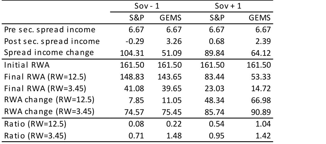
To assess the balance-sheet efficiency of the alternative capital structures, we calculate a Benefit-to-Cost (BTC) ratio. The BTC ratio is defined as the percentage reduction in RWAs divided by the percentage reduction in net spread income:
To calculate the percentage reduction in RWAs, the initial portfolio risk weight is set at 161.5%. It is calculated as the exposure-weighted average of the country-specific risk weights applicable to the loans in the stylised portfolio.
In calculating the post-securitisation RWA, we assume that all rated debt tranches are transferred to investors and that only the residual equity tranche is retained by the MDB. The post-securitisation RWA therefore depends solely on the thickness of the retained equity tranche and the risk weight applied to it. No additional RWA is included for a retained mezzanine tranche or an insurance counterparty.
Two alternative equity-tranche treatments are considered. Under the first, a 1,250% risk weight is applied to the retained equity exposure. This represents the standard treatment of an unrated or first-loss securitisation exposure. Under the second, a 345% risk weight is applied. This represents the alternative capped treatment considered in the analysis.
The percentage RWA reduction is calculated as
where is the equity-tranche risk weight (12.5 or 3.45); is the proportion of the equity-tranche retained by the MDB (assumed to be 1); denotes the equity-tranche thickness; and is the pre-securitisation portfolio risk weight (1.615). The cost of the transaction is measured by the percentage reduction in net spread income. Before securitisation, net spread income is calculated from the weighted-average spread on the portfolio after deducting the MDB’s funding spread, recurring transaction costs and expected losses. For the current calculation we assume zero overhead costs and no insurance premium. The resulting annual net spread is then multiplied by the WAL of the underlying portfolio. Following securitisation, the MDB no longer receives the spread income associated with the transferred rated tranches. Its remaining income consists of the expected residual return on the retained equity tranche. This is calculated using the equity tranche’s expected spread and expected WAL. The percentage reduction in net spread income is calculated as:
Where and are the weighted average spread and Weighted Average Life (WAL) for the underlying loan pool. and are the expected equity spread and equity tranche WAL. and are the MDB funding spreads at the tenors corresponding to the equity tranche and loan pool WALs. denotes the weighted average expected loss for the loan pool. Note that the is derived from the expected IRR. Because simulated defaults and recoveries directly reduce the interest and principal cash flows received by the retained equity tranche, the expected loss allocated to that tranche is already incorporated into . EL is, therefore, not deducted separately from the post-securitisation equity spread. In the current study, the funding spread is assumed to be 45 bps over SOFR. The 1-year EL is assumed to equal 0.55% of the portfolio par value. The results for the four scenarios are shown in Table 4.4.
Show as data
| Sov - 1 | Sov + 1 | |||
|---|---|---|---|---|
| S&P | GEMS | S&P | GEMS | |
| Pre sec. spread income | 6.67 | 6.67 | 6.67 | 6.67 |
| Post sec. spread income | -0.29 | 3.26 | 0.68 | 2.39 |
| Spread income change | 104.31 | 51.09 | 89.84 | 64.12 |
| Initial RWA | 161.50 | 161.50 | 161.50 | 161.50 |
| Final RWA (RW=12.5) | 148.83 | 143.65 | 83.44 | 53.33 |
| Final RWA (RW=3.45) | 41.08 | 39.65 | 23.03 | 14.72 |
| RWA change (RW=12.5) | 7.85 | 11.05 | 48.34 | 66.98 |
| RWA change (RW=3.45) | 74.57 | 75.45 | 85.74 | 90.89 |
| Ratio (RW=12.5) | 0.08 | 0.22 | 0.54 | 1.04 |
| Ratio (RW=3.45) | 0.71 | 1.48 | 0.95 | 1.42 |
5. Conclusion
This study demonstrates the economic impact on MDB securitisations of the views that rating agencies take of the underlying loan credit quality.
The assumptions the agencies adopt on MDB loans, as exemplified by Standard & Poor’s, are extremely conservative as regards LGD rates. For the higher rated tranches, the agency on which we focus here (which has the most transparent methodology of the three global agencies), Standard & Poor’s, assumes LGDs for corporate exposures in Group C countries (which includes most countries represented in MDB portfolios) in excess of 81.52% (see Table A4.2 in Appendix 4). This LGD assumed by the agency is a stressed version of a base LGD of 65.8%. GEMs data suggests the base LGD is 27.1%.
A comparison of the three global rating agencies’ LGD assumptions for the same stylised emerging market portfolio shows that the conservatism is not specific to Standard & Poor’s. Fitch assumes an LGD of 96.9% for the ‘AAA’ stress, implying almost no recovery, against 81.5% under Standard & Poor’s, and the two agencies’ base case LGDs are 68.8% and 65.8% respectively. Moody’s, which applies the same LGD assumptions to emerging market and developed market obligors, implies a mean LGD of 49.5%. All three are well above the 27.1% average LGD observed in the GEMs data for MDB private-sector lending. The divergence between Moody’s region-neutral treatment and the jurisdiction-based assumptions of Standard & Poor’s and Fitch suggests that the evidence for materially higher LGDs on emerging market obligors is less clear-cut than the latter agencies’ assumptions imply. This strengthens the case for MDBs to present their own recovery data to the agencies.
It is harder to observe directly how the agencies approach the mapping exercises that they employ to convert MDB internal ratings into the usual AAA to CC alpha-numeric scale. This mapping determines how conservative or otherwise the agency is as regards PDs. It is through this mapping that the benefits of MDBs’ preferred creditor status and reduced transfer risk would be reflected.
In the calculations presented in this study, we presume that the agencies are influenced by the sovereign rating cap that they typically apply and, hence, assign a rating to corporate loans on average 1 notch below the corresponding sovereign rating. Analysis we have performed on public data from IFC suggests that MDB’s historical default rates are consistent with a 1-notch-above sovereign grading of corporate loans. These are modelling assumptions, but benchmarking against the sovereign is, in our view, also the most obvious check an agency would apply to an MDB’s mapping, given the importance of the sovereign rating ceiling for loans in EMDEs.
Under the assumptions just described about LGDs and PDs, we show that a CLO with the tranching devised in Section 4 receives an IRR spread over SOFR of 11% compared to a spread close to zero under the agency assumptions. On the BTC ratio that many MDBs now employ to measure the efficiency of risk transfers, the reasonable PD and LGD assumptions imply a BTC ratio of 1.4 compared to 0.7 under the agency assumptions.
These results rest on a stylised pool, on modelling assumptions about the rating of loans relative to the sovereign, and on illustrative tranche spreads. They reflect Standard & Poor’s methodology, whose tools are publicly available; Fitch and Moody’s could reach different conclusions on the same pool. The structures derived are model-supported capital structures rather than structures that would necessarily receive the stated ratings. The results should therefore be read as indicating the direction and approximate scale of the effect of agency assumptions on deal economics rather than as estimates of any particular transaction. The conservatism of the agencies is not surprising. For a new asset class with limited deal volume, generic and conservative assumptions are inevitable. It is for MDBs to make the case, based on statistical evidence from their own loan performance data, for a different treatment.
What would be necessary for the ratings agencies to change their methodologies. Rating agencies are commercial organisations that have both pecuniary and reputational motivations in deciding whether to make methodology changes:
(i) If agencies think the market will be large enough for them to make money, they will be more willing to consider modifications in their approaches. Otherwise, they will stick to standard approaches.
(ii) Agencies will only be willing to make changes if they are presented with evidence. This is appropriate: methodologies should change only to the extent that a proper case is made on the basis of statistical evidence on the credit performance of the loans.
To bring about changes in agency methodologies, therefore, MDBs need to generate sufficient deal volume to make it commercially interesting to the agencies and they must also provide convincing evidence. Evidence does not simply mean raw data but also apposite analysis. The issues on which agencies will want evidence are:
(a) Is there lower transfer risk in MDB loans than public bonds or loans from commercial banks justifying the idea that MDB loans be rated in a mapping exercise as higher than the corresponding sovereign (b) How do LGDs behave in stressed EMDE credit market conditions. The current extreme LGDs employed by the agencies for NSO loans in EMDE countries are justified by the notions that recoveries are low when defaults are common. This argument can be taken to unrealistic extremes when no good evidence is available.
The data of the MDB undertaking a transaction will be central to any mapping exercise. The pooled GEMs statistics provide valuable market-level evidence but conceal significant variation in credit performance across MDBs, and a prudent agency will wish to understand the history of the specific originator. MDBs with long runs of data, such as IFC or AfDB, should be able to support mappings on which they and the agencies can rely. MDBs with shorter histories will have to accept the additional conservatism the agencies will naturally and correctly require until their records lengthen. In all cases, progress is most likely to come through dialogue with the agencies, transparency and systematic provision of data.
This study is aimed at:
• Senior MDB and DFI management and shareholders, for whom the importance of rating agency methodologies for the development of MDB-loan securitisation markets may not be fully apparent.
• The rating agencies themselves which, we hope, will be open to reconsidering aspects of their approaches if appropriate evidence is provided.
Correctly calibrating risk and rating models for EMDE risk is an initial step in opening these debt markets to a broader cross-section of developed country investors.
References
Fitch (2023) “CLOs and Corporate CDOs Rating Criteria,” July, available at: https://www.fitchratings.com/research/structured-finance/clos-corporate-cdos-rating-criteria-21-07-2023
Fitch (2024) “Supranationals Rating Criteria,” October, available at: https://www.fitchratings.com/research/sovereigns/supranationals-rating-criteria-03-10-2024
Fitch (2025) “Global Structured Finance Rating Criteria,” December, available at: https://www.fitchratings.com/research/structured-finance/global-structured-finance-rating-criteria-05-12-
Galizia, Federico, William Perraudin, Andrew Powell, and Timothy Turner (2021) “Risk Transfer for Multilateral Development Banks: Obstacles and Potential,” available at: https://publications.iadb.org/publications/english/document/Risk-Transfer-for-Multilateral-Development- Banks-Obstacles-and-Potential.pdf
Global Emerging Markets Risk Database (2025) “Default and Recovery Statistics Private Lending 1994-2024,” October, available at: https://www.gemsriskdatabase.org/recent-publications/
International Finance Corporation (2024) “IFC Portfolio Default Rate Analysis,” March, available: https://www.ifc.org/en/insights-reports/2024/ifc-portfolio-default-rate-analysis
Moody’s (2024) “Corporate Synthetic CDOs,” May, available at: https://ratings.moodys.com/rmcdocuments/420174
Moody’s (2025) “Rating Symbols and Definitions,” December, available at: https://www.moodys.com/research/doc--PBC_79004
Moody’s (2026) “Multilateral Financial Institutions,” June, available at: https://ratings.moodys.com/rmcdocuments/468058
Risk Control (2024) “Innovative Deals in Development Finance: Originate to Demonstrate (O2D),” 24-66a, August, available at: https://www.riskcontrollimited.com/insights/innovative-deals-in-development-financeoriginate-to-demonstrate-o2d/
Risk Control (2025) “Regulatory Data Requirements for Securitisation Investors,” January 24-126a, available at: https://www.riskcontrollimited.com/wp-content/uploads/2025/01/Regulatory-Data-Requirements-for- Securitisation-Investors-24-126a-06-01-25-v23.pdf
Risk Control (2026a) “Ex Post Evaluation of Financial Demonstration Effects,” Research Report, May.
Risk Control (2026b) “IFC’s EMSP 2025-1: Implications for MDBs and Market Building,” Research Report, July.
Risk Control (2026c) “Market Awareness of MDB Securitisations,” Research Report, August.
Risk Control (2026d) “How to Make a Success of MDB Securitisation,” Research Report, August.
Standard & Poor’s (2014) “Mapping A Third Party's Internal Credit Scoring System To S&P Global Ratings' Global Rating Scale,” May, available at: https://www.spglobal.com/ratings/en/regulatory/article/- /view/sourceId/8563856
Standard & Poor’s (2019) “Global Methodology And Assumptions For CLOs And Corporate CDOs,” June, available at: https://www.spglobal.com/ratings/en/regulatory/article/-/view/sourceId/11020014
Standard & Poor’s (2020) “Global Framework For Payment Structure And Cash Flow Analysis Of Structured Finance Securities,” December, available at: https://www.spglobal.com/ratings/en/regulatory/article/- /view/sourceId/11734324
Standard & Poor’s (2024) “Risk-Adjusted Capital Framework Methodology,” April, available at: https://www.spglobal.com/ratings/en/regulatory/article/-/view/sourceId/13062752
Standard & Poor’s (2025) “Multilateral Lending Institutions And Other Supranational Institutions Ratings Methodology,” October, available at: https://www.spglobal.com/ratings/en/regulatory/article/- /view/sourceId/101641447
Standard & Poor’s (2026a) “Recovery Rating Criteria For Corporate Issuers,” March, available at: https://www.spglobal.com/ratings/en/regulatory/article/-/view/sourceId/101672470
Standard & Poor’s (2026b) “Methodology For Rating Structured Finance Securities Above The Sovereign,” April, available at: https://www.spglobal.com/ratings/en/regulatory/article/-/view/sourceId/101667797
Appendix 1: Standard & Poor’s Securitisation Rating Approaches
A1.1 Adjusted Total Loss Approach Under the adjusted total loss approach, Standard & Poor’s uses the RACF as the basis for assessing the magnitude of risk transfer. For retained risk, Standard & Poor’s states that the equity tranche is typically assigned a 1250% risk weight. The risk weight applied to the retained mezzanine and senior tranches are summarised in Table 2.1 and weighted according to the level of credit enhancement needed to survive the relevant stress. Standard & Poor’s own example indicates that if losses are fully absorbed by junior and mezzanine protection, the retained senior tranche could be inferred at about ‘A’ and assigned a 50% risk weight. They also note that more severe stress levels could be considered under the CDO criteria in the RACF.
If a transferred tranche is fully funded and collateral is segregated in a way that removes counterparty uncertainty, Standard & Poor’s can treat the corresponding risk as effectively removed. If the protection depends on the offtaker’s promise to pay, the residual exposure instead depends on the credit quality of the offtaker or guarantor. Guaranteed tranches can receive risk substitution treatment if the guarantee meets the standard conditions of timeliness, irrevocability, and unconditionality.
A1.2 CLO/corporate CDO criteria The rating input provides information about the corporate issuer’s creditworthiness and is determined based on the hierarchy of available rating information
A1.3 CDO mapping criteria For the third CDO mapping criteria Standard & Poor’s (2014) establishes a three-step process:
1. Collection of a statistically significant sample of obligors for which both an internal credit score and a Standard & Poor’s rating or credit estimate exist.
2. Review of the institution's underwriting and credit-approval processes to confirm that scores are
independently and consistently assigned. 3. Performance of a statistical analysis to establish a correspondence table. The statistical procedure works as follows. Each obligor in the sample is assigned the five-year cumulative PD corresponding to its Standard & Poor’s global rating level. For each internal score bucket, the sample mean default rate and standard deviation are calculated, followed by estimation of the one-tailed upper 95% confidence bound for the population mean: , where is the sample mean default rate, is the sample
standard deviation, is the number of obligors in that score bucket, and is the 95th percentile of the t-distribution with −1 degrees of freedom. This upper bound is then mapped back to Standard & Poor’s rating scale; where it falls between two rating levels, the more conservative (lower) rating is assigned. A monotonicity constraint is finally applied to ensure the resulting correspondence table preserves the rank ordering of the rating scale.
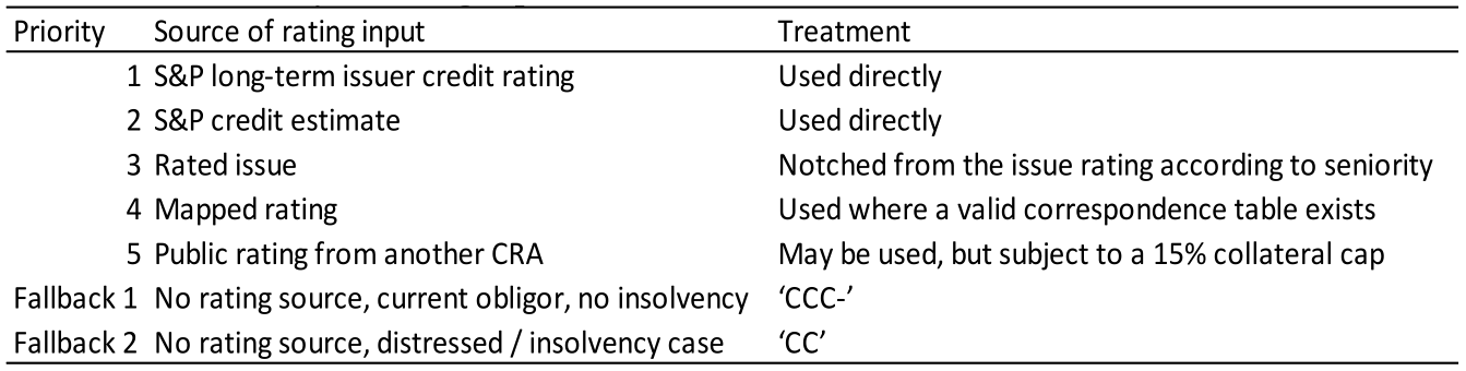
Show as data
| Priority | Source of rating input | Treatment |
|---|---|---|
| 1 | S&P long-term issuer credit rating | Used directly |
| 2 | S&P credit estimate | Used directly |
| 3 | Rated issue | Notched from the issue rating according to seniority |
| 4 | Mapped rating | Used where a valid correspondence table exists |
| 5 | Public rating from another CRA | May be used, but subject to a 15% collateral cap |
| Fallback 1 | No rating source, current obligor, no insolvency | ‘CCC-’ |
| Fallback 2 | No rating source, distressed / insolvency case | ‘CC’ |
Appendix 2: Fitch’s Securitisation Rating Approach
Junior-only synthetic securitisations receive the same treatment as the FLP guarantee. FLP guarantees are treated as a form of loss-absorbing support added to usable capital in the FRA ratio. The recognised amount is first reduced by a haircut reflecting the credit quality of the guarantor as summarised in Table A2.1.
Fitch uses the issuer rating and the term of the asset as the main inputs to determine PD. Table A2. 2 summarise the preferred order of the rating input sources.

Show as data
| Guarantor rating | AAA | AA | A | BBB |
|---|---|---|---|---|
| Recognised amount in usable capital | 100 | 80 | 70 | 50 |
Note: All values are expressed as percentages.
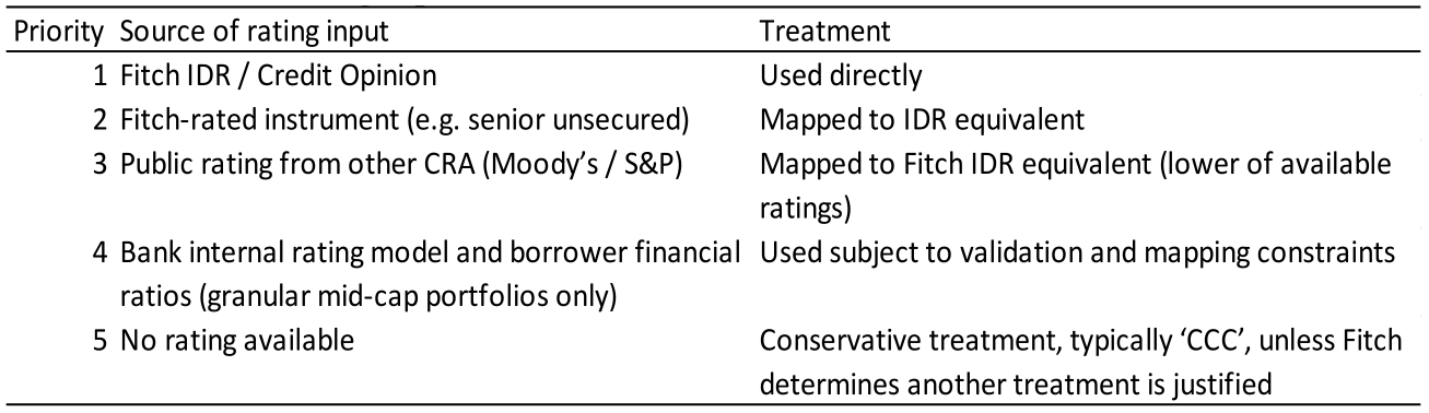
Show as data
| Priority | Source of rating input | Treatment |
|---|---|---|
| 1 | Fitch IDR / Credit Opinion | Used directly |
| 2 | Fitch-rated instrument (e.g. senior unsecured) | Mapped to IDR equivalent |
| 3 | Public rating from other CRA (Moody's / S&P) | Mapped to Fitch IDR equivalent (lower of available ratings) |
| 4 | Bank internal rating model and borrower financial ratios (granular mid-cap portfolios only) | Used subject to validation and mapping constraints |
| 5 | No rating available | Conservative treatment, typically 'CCC', unless Fitch determines another treatment is justified |
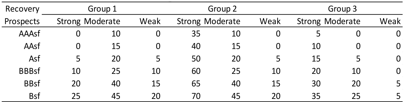
Show as data
| Recovery Prospects | Group 1 Strong | Group 1 Moderate | Group 1 Weak | Group 2 Strong | Group 2 Moderate | Group 2 Weak | Group 3 Strong | Group 3 Moderate | Group 3 Weak |
|---|---|---|---|---|---|---|---|---|---|
| AAAsf | 0 | 10 | 0 | 35 | 10 | 0 | 5 | 0 | 0 |
| AAsf | 0 | 15 | 0 | 40 | 15 | 0 | 10 | 0 | 0 |
| Asf | 5 | 20 | 5 | 50 | 20 | 5 | 15 | 5 | 0 |
| BBBsf | 10 | 25 | 10 | 60 | 25 | 10 | 20 | 10 | 0 |
| BBsf | 20 | 40 | 15 | 65 | 40 | 15 | 30 | 20 | 5 |
| Bsf | 25 | 45 | 20 | 70 | 45 | 20 | 35 | 25 | 5 |
Note: All values are expressed as percentages. Full recovery tables are provided in Fitch (2023) Appendix 4.
Appendix 3: Moody’s CLO Methodology
A base PD is inferred from the reference entity rating and the tenor of the exposure using Moody’s idealised default probability tables. Table A3. 1 summarise the preferred order of the rating input sources. Further rating input adjustments might be applied as shown in Table A3. 2.
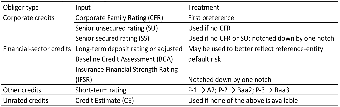
Show as data
| Obligor type | Input | Treatment |
|---|---|---|
| Corporate credits | Corporate Family Rating (CFR) | First preference |
| Senior unsecured rating (SU) | Used if no CFR | |
| Senior secured rating (SS) | Used if no CFR or SU; notched down by one notch | |
| Financial-sector credits | Long-term deposit rating or adjusted Baseline Credit Assessment (BCA) | May be used to better reflect reference-entity default risk |
| Insurance Financial Strength Rating (IFSR) | Notched down by one notch | |
| Other credits | Short-term rating | P-1 → A2; P-2 → Baa2; P-3 → Baa3 |
| Unrated credits | Credit Estimate (CE) | Used if none of the above is available |
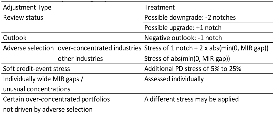
Show as data
| Adjustment Type | Treatment |
|---|---|
| Review status | Possible downgrade: -2 notches |
| Review status | Possible upgrade: +1 notch |
| Outlook | Negative outlook: -1 notch |
| Adverse selection: over-concentrated industries | Stress of 1 notch + 2 x abs(min(0, MIR gap)) |
| Adverse selection: other industries | Stress of abs(min(0, MIR gap)) |
| Soft credit-event stress | Additional PD stress of 5% to 25% |
| Individually wide MIR gaps / unusual concentrations | Assessed individually |
| Certain over-concentrated portfolios not driven by adverse selection | A different stress may be applied |
Note: Here, MIR refers to Market-Implied Ratings. The detailed tables for soft credit-event stress are reported in Exhibit 7 of Moody’s (2024).
Appendix 4: Demo Portfolio Assumptions
Standard & Poor’s gives priority to an asset’s own recovery rating and then to information from a more-seniorranking asset. Since neither type of information is available for the stylised portfolio, recoveries are determined using Standard & Poor’s asset-type framework. This framework differentiates recoveries according to whether the exposure is a loan or bond, its seniority and security, and the recovery group of the borrower’s country.
The allocation is based on a target distribution consisting of senior secured first-lien loans, senior secured covenant-lite loans or senior secured bonds, and mezzanine, second-lien or senior unsecured loans, as shown in Table A4.1.
The recovery assumption for each exposure is then determined from the combination of its assigned recovery type, country recovery group, and the rating stress applied to the tranche under consideration. Standard & Poor’s assumptions vary across rating stresses, with lower recovery rates generally applied under the more severe stresses associated with more highly rated liabilities.
A second recovery framework is constructed using historical recovery information from the GEMs privatelending database. The GEMs data for 1994–2024 report an average recovery rate of 72.9%, equivalent to an LGD of 27.1%. This recovery rate is used as the anchor for the CCC stress case.
Recovery rates for the stronger liability-rating stresses are derived by applying the relative stress pattern in S&P’s assumptions for senior secured first-lien covenant-lite loans in Group A countries. Under the S&P framework, the corresponding recovery rates are 41%, 46%, 49%, 53%, 63% and 67% for the AAA, AA, A, BBB, BB and B/CCC stresses, respectively. The GEMs-based recovery rate for stress level s is therefore calculated as:
The recovery rate assumptions for the two cases are summarised in Table A4.2.
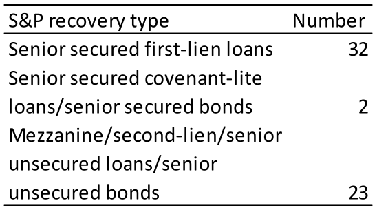
Show as data
| S&P recovery type | Number |
|---|---|
| Senior secured first-lien loans | 32 |
| Senior secured covenant-lite loans/senior secured bonds | 2 |
| Mezzanine/second-lien/senior unsecured loans/senior unsecured bonds | 23 |

Show as data
| AAA | AA | A | BBB | BB | B | CCC | |
|---|---|---|---|---|---|---|---|
| Standard & Poor's | 18.48 | 20.72 | 25.72 | 27.96 | 31.58 | 34.20 | 34.20 |
| GEMS | 44.61 | 50.05 | 53.31 | 57.67 | 68.55 | 72.90 | 72.90 |
Note: All values are expressed as percentages.
Notes
[1] This study is an independent research paper prepared by Risk Control. The analysis and conclusions it contains do not necessarily represent the views of FCDO or SECO which commissioned the research.
[2] Galizia, Perraudin, Powell and Turner (2021) make the case for more extensive use of securitisation by MDBs. © Copyright Risk Control Limited 2026
[3] A natural question is whether the features that produced this performance remain effective after the risk transfer. MDBs typically retain no less than 50% of securitised loans (as was the case, for example, in AfDB’s Room2Run (R2R)).
[4] A uniform relationship to the sovereign rating does not capture differences between, for example, a bank, an export- oriented corporate with hard currency revenues, a domestic utility and a limited-recourse infrastructure project, whose dependence on sovereign payments, regulations and access to foreign currency differs. A more granular treatment would be appropriate in a live transaction but lies beyond the scope of this study.
[5] Standard & Poor’s notes that synthetic risk transfer may result in a less complete transfer of risk than a true sale transaction, as the MLI may substitute exposure to the underlying assets with a concentrated exposure to the protection provider. This counterparty risk may, however, be mitigated where the transferred tranches are fully collateralised upfront.
[6] Because the RACF is calibrated to an ‘A’-level stress, this approach principally supports an assessment of whether a tranche has sufficient credit enhancement to survive an ‘A’ stress.
[7] Under the RACF-based approach, for example, a senior tranche may be inferred to have an ‘A’ rating where the junior and mezzanine tranches are sufficient to absorb the full RACF-derived ‘A’-stress loss. The CDO criteria permit a more differentiated assessment because they consider stress scenarios corresponding to a range of rating levels. © Copyright Risk Control Limited 2026
[8] See Standard & Poor’s (2019) Table 11 for the tranche rating quantile.
[9] See Standard & Poor’s (2019) Table 3 for the full calibrated table provides discrete tenors from 1 to 10 years.
[10] See Standard & Poor’s (2026b), Tables 13–15, for recovery assumptions based respectively on asset-specific recovery indicators, pari passu recovery indicators and standard assumptions by asset type, seniority, security and country grouping.
[11] See Standard & Poor’s (2026a) for the detailed corporate recovery rating methodology. Standard & Poor’s first estimates the recovery percentage for each debt instrument, rounds the estimate down to the nearest 5%, and then maps the rounded recovery percentage to a recovery rating from ‘1+’ to ‘6’. Table 1 of the methodology provides the mapping between recovery percentage ranges and recovery ratings.
[12] See Standard & Poor’s (2026b), Appendix C, Table 10.
[13] Details of the Fitch IDR equivalency map can be found in Fitch (2023) Appendix 5.
[14] The full PD term structure can be found in Fitch (2023) Appendix 1.
[15] See Fitch (2023), p. 43, for the list of countries included in each of the three groups.
[16] See Fitch (2023) Appendix 4 Asset-Specific Recovery Rate Assumptions table.
[17] See Fitch (2023) Appendix 4 Recovery Rate Assumptions table.
[18] See Moody’s (2025) section Idealized Probabilities of Default and Expected Losses.
[19] The GEMs-based framework is itself a stressed MDB recovery case: the GEMs historical average recovery rate is applied only at the CCC stress and is scaled down for higher rating stresses in line with the Standard & Poor’s stress pattern (see Appendix 4). A fuller bridge between the historical evidence and the recovery assumptions would present three cases side by side: published agency recoveries, historical MDB recoveries and a stressed MDB recovery rate. To keep the presentation focused on a single key table we do not do this here.
[20] Recovery timing matters as well as the ultimate level of recovery. An ultimate recovery of 70% received after several years provides less protection than a prompt recovery of the same amount, since a prolonged workout may produce interest shortfalls, pressure on overcollateralisation tests and a longer WAL. In an EMDE infrastructure loan portfolio, there is a low chance of a quick recovery.
[21] This is the same argument that justifies the use of stressed LGDs in Basel regulatory capital calculations. Note: All values are expressed as percentages. LGDs are exposure- weighted across the stylised portfolio described in Sub-section 4.2, using rating agency’s standard assumptions. Moody’s does not tier LGDs by rating stress; its mean portfolio LGD is 49.5%, with a standard deviation of 25% to 30% depending on asset security.
[22] AAA spreads are generally observed in the range of approximately 100 to 250 bps, while AA and A tranches are typically in the range of 150 to 400 bps. BBB tranches span a wider range of approximately 250 to 700 bps. BB tranches show the greatest volatility, with spreads ranging from around 600 bps in stable periods to approximately 1,600 to 1,800 bps during stressed periods.