

In standard ratings-based models for analysing credit portfolios and pricing credit derivatives, it is assumed that defaults and recoveries are statistically independent. This paper presents evidence that aggregate quarterly default rates and recovery rates are, in fact, negatively correlated. Using Extreme Value Theory techniques, we show that the dependence affects the tail behaviour of total credit loss distributions and leads to higher VaR measures. * Barclays Capital, yen-ting.hu@barclayscapital.com ** Imperial College, London and Risk Control Limited, wperraudin@riskco.co.uk
Research Paper
The Dependence of Recovery Rates and Defaults
Date:2006 Reference Number:6/1
The Dependence of Recovery Rates and Defaults
Yen-Ting Hu* and William Perraudin**
This version: February 2006
1 Introduction
In the standard ratings-based credit risk model developed by Gupton, Finger and Bhatia (1997), it is assumed that recoveries on defaulted exposures are random outcomes, independent of default events. A similar independence assumption is made in the pricing models of Jarrow, Lando and Turnbull (1997) and Kijima and Komoribayashi (1998). While the assumption is a sensible starting point for analysis, it might be seen as questionable.
This paper uses Moody’s data for January 1971 to January 2000 to investigate the dependence between quarterly, aggregate recovery and default rates. Recovery rates are defined as the ratio of the market value of the bonds to the unpaid principal, one month after default, averaged across the bonds that default in a given quarter. Default rates are defined as the fraction of bonds that default in a quarter to the number of bonds rated at the start of the quarter.
Our study is complicated by the fact that the pool of bond issues rated by Moody’s changes over time. For example, utilities made up over 50% of Moody’s-rated firms in the early 1970s but this percentage had fallen to less than 10% by 1999. Since different industries have very different recovery rates, changes in the industry breakdown of the rated pool may generate apparent volatility in recovery rates in time series samples. Since this volatility is unlikely to be related to aggregate defaults, it will make aggregate default and recovery rates appear less correlated than they actually are.
To cope with the time-variation in the sample of recoveries, as the first stage of our analysis, we “standardise” the recovery data. We achieve this by estimating a statistical model of recovery rates in which issue-characteristics including industry and seniority appear as regressors. Using the model, we are then able to calculate what the recoveries would have been for each obligor in the sample if that obligor had possessed certain standard characteristics. The characteristics of our reference issue type are those of a senior unsecured, US-industrial issue with no backing by another organisation.
The statistical model we employ to standardise the recoveries data has some independent interest. There is a substantial empirical literature on bond and loan recoveries (see Hickman (1958), Fons (1994), Asarnow and Edwards (1995), Carty and Lieberman (1996), and Altman and Kishore (1996) amongst others). But, all the published studies have limited themselves to comparisons of mean recovery rates for different defaulted issues with different characteristics. This has the drawback that the marginal impact of particular characteristics cannot be determined. In contrast, in this study, we perform multivariate regressions so the effect of changing one variable while holding others constant is apparent.
Given our estimates of standardised aggregate recovery rates and default rates, we study their dependence by calculating correlations between quarterly recovery rates and default rates for issues by US-domiciled obligors, over different time periods. We conclude that typical correlations for post 1982 quarters are –22%. If the period 1971-2000 is considered, typical correlations are -19%.
However, what often matters for credit risk measures and capital is not correlation, but the degree of dependence between extreme realisations of default rates and recovery rates. To study this dependence, we examine the total credit losses faced by an investor who, in each quarter, holds equal dollar amounts in each of the bonds rated by Moody’s. We define total credit losses as the default rate in the quarter times one minus the average recovery rate in the quarter. This corresponds to a default-mode notion of credit losses, as losses associated with declines in credit standing short of default do not contribute to this measure of losses.
We employ non-parametric techniques to estimate the density and the tail of the distribution of total credit losses. We do this for actual losses and for loss data in which we have artificially eliminated any dependence by randomly selecting default rate-recovery rate pairs to form a simulated total loss rate. We then compare the distribution of losses with and without dependence, focussing in particular on Value at Risk (VaRs) statistics.
The techniques we employ for estimating total loss VaRs are drawn from the recent Extreme Value Theory literature on tail estimation with small samples. This is appropriate as we have between 71 and 84 quarterly observations depending on which sub-sample we employ. The approach we take follows that of Huisman, Koedijk, Kool and Palm (2001) who suggest a regression technique for estimating tail indices of distributions in small samples. Kiesel, Perraudin and Taylor (2001a) present an extension and apply these techniques to emerging market benchmark bond returns.
The structure of the paper is as follows. Section 2 describes the data and provides statistics on recovery rates. Section 3 described our technique for standardising recoveries and presents regression results on how recovery rates vary for defaults on bonds with different characteristics. Section 4 reports correlation measures for recovery and default rates. Section 5 uses non-parametric techniques to estimate the distribution of total credit losses with and without dependence between recovery rates and default rates. Section 6 concludes.
2 Background information on the recoveries data
2.1 Data description
The data we employ are the “Moody’s Corporate Bond Default Database” provided by Moody’s Credit Risk Management Services. This database contains the credit experience and characters of all Moody’s-rated, long-term bond defaults from financial institutions, industrials, transportations, utilities and sovereigns. Moody’s define the recovery rate on a defaulted bond issue as the ratio of market value of the defaulted bond to unpaid principal one month after the default date.[1] Default is defined as the occurrence of one of the following events: a) missing or delaying interest and/or principal, b) filing for bankruptcy or legal receivership and c) there is a distressed exchange where the exchange package is apparently helping the borrower avoid default.
The dataset contains default data in the period between 1 January 1970 and 5 January 2000. However, in 1970, there were total 48 defaulted issues, 42 of which defaulted on the same date, 21 June 1970. Due to the fact that the total number of Moody’s rated bonds at the time are relative small, around 2000 issues, these highly concentrated default events accounted for more than 2% of the total number of rated bonds. To avoid possible miss-representative of the 1970 data, we decide to concentrate our analysis on the data between 1 January 1971 and 5 January 2000.
Having dropped the data in 1970, the dataset then contain 1422 observations in total. However for many of these, at least one of the variables we wished to use in our analysis is missing. The variable that is missing most often is the recovery rate itself (311 missing observations), presumably reflecting the fact that, it may be difficult to obtain observations of market values of defaulted bonds. Perhaps surprisingly, a fairly large fraction of missing observations occur towards the end of the sample period, although there are missing observations throughout the three decades. Once we have removed all observations containing missing values, the number of recovery rate observations that remains is 958.
Moody’s classify issuers into 11 broad categories: transportation (72 observations), industrial (728), insurance (12), banking (25), public utility (57), finance (11), thrifts (20), securities (2), real estate (8), other non-bank (15), and sovereign (8). Since we intend to use industry dummies as regressors and some categories contained too few observations to be usable, we aggregate further into transportation (72), industrial (728), public utility (57), banking and thrifts (45), others (48) and sovereign (8).
Similarly, Moody’s classify issues by seniority into the categories: senior secured (105), senior unsecured (327), senior subordinated (78), subordinated (437), and junior subordinated (11). We aggregate the junior subordinated and subordinated categories in order to obtain enough observations.
Finally, Moody’s supply a country code for the domicile of each bond’s issuer. We aggregate these to obtain broad geographical categories: US (910), emerging markets countries (22), non-US OECD (23) and off shore banking centres (3).
1 This definition might be questioned as entitlement in default settlements is generally based on unpaid principal plus accrued interest. However, the implied bias is unlikely to be substantial.
Greece and Mexico are treated as emerging market countries rather than being included as non-US OECD.
2.2 Recovery distributions
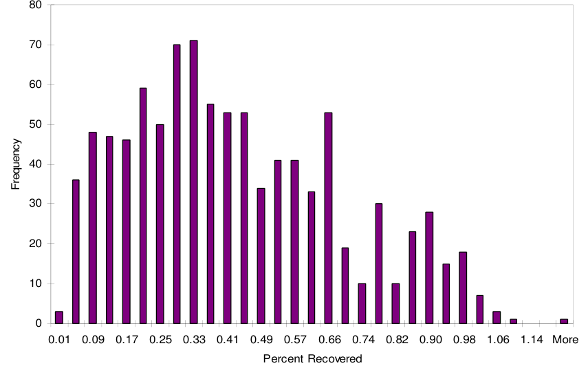
The empirical distribution of recoveries for all 958 observations in our sample is shown in Figure 1. The empirical distribution appear approximately regular, by which we mean roughly unimodal and somewhat but not grossly skewed. This is in contrast to the highly skewed and bimodal empirical bank loan recovery distributions shown in Asarnow and Edwards (1995). The difference reflects the fact that the latter is based on discounted cash recoveries rather than bond prices just after default.
Table 1 shows mean recovery rates in percent estimated from our data and those reported by past studies. The average recovery rates we obtain are similar to those found in the literature, especially to those obtained by Carty and Lieberman (1996) whose bond dataset has much overlap with the one employed here.
Table 2 shows the means and volatilities (standard deviations) of recovery rates for different industry and geographic categories. As past studies have found, our recovery data is highly sensitive to the industry of the issuer. Utilities have a mean recovery rate of 70% while for bank and thrift issuers, the recovery rates are 23% and 26% respectively. The domicile of the bond issuer affects the mean recovery rate less, however. The volatilities of recovery rates do not bear any very obvious relation to the level of the means.
3 Extracting Standardised Recoveries
3.1 Recovery rate regressions
As explained in the Introduction, analysing the dependence of recovery and default rates is complicated by the fact that the pool of obligors rated by Moody’s has evolved over time. The fractions of non-US domiciled issuers and banks in the Moody’s rated pool have grown from 5% and 0.7% to 59% and 45% from 1971 to
1999. At the same time, the fraction of utilities has fallen from 61% to 7%. Since recovery rates depend on the characteristics of the bond issue, these changes have led to a significant evolution in average recovery rates that in a time series will appear to be additional volatility. Since this volatility is likely to be uncorrelated with changes in default rates, it will bias down estimates of correlation between recovery and default rates.
To overcome this difficulty, before examining the dependence between default rates and recovery rates, we filter the recoveries data by estimating “standardized” recovery rates for a particular type of bond issue. To accomplish this, we estimate a statistical model of recoveries in which characteristics of the bond issue and of the issuer appear as conditioning variables or regressors. Formally, we suppose that recoveries on the ith default, Ri , may be expressed as a regression on an N-vector of
variables X i . Ri = Xiβ+εi (3.1)
Here, β is an N-vector of parameters to be estimated and εi is an error term with a
mean of zero conditional on X i .
Using this model, we can calculate what recovery rate the defaulted issue would have if it were the recovery on a defaulted issue of a given reference type. Specifically, if βˆ is the estimated parameter vector and εˆi is the fitted residual, then
* Ri is the standardized residual for the ith observation, where: * * ) ) Ri = X β+εi (3.2)
* and X is the vector of characteristics of the reference issue type.
The variables we include in the X i vector include:
1. Industry dummies for the categories: (i) transport, (ii) public utility, (iii) banking and thrifts, (iv) sovereigns, (v) others non-industrials. The category omitted so as to obtain identification is that of industrials.
2. Domicile dummies for the categories: (i) emerging markets, (ii) non-US OECD, (iii) off-shore banking center. The omitted category is US domicile.
3. Seniority dummies for the categories: (i) senior secured, (ii) senior subordinated, (iii) subordinated and junior subordinated. The omitted category is senior unsecured.
4. A dummy reflecting whether the issuer has support from some other organization.
All the dummy variables are demeaned so instead of equaling either one or zero, they equal one or zero minus the fraction of observations for which the original dummy was unity.
Our reference bond issue is a senior unsecured bond issued by a US-domiciled industrial with no support by another entity. The entries in the reference vector of
* regressors, X , are chosen accordingly.
3.2 Regression results
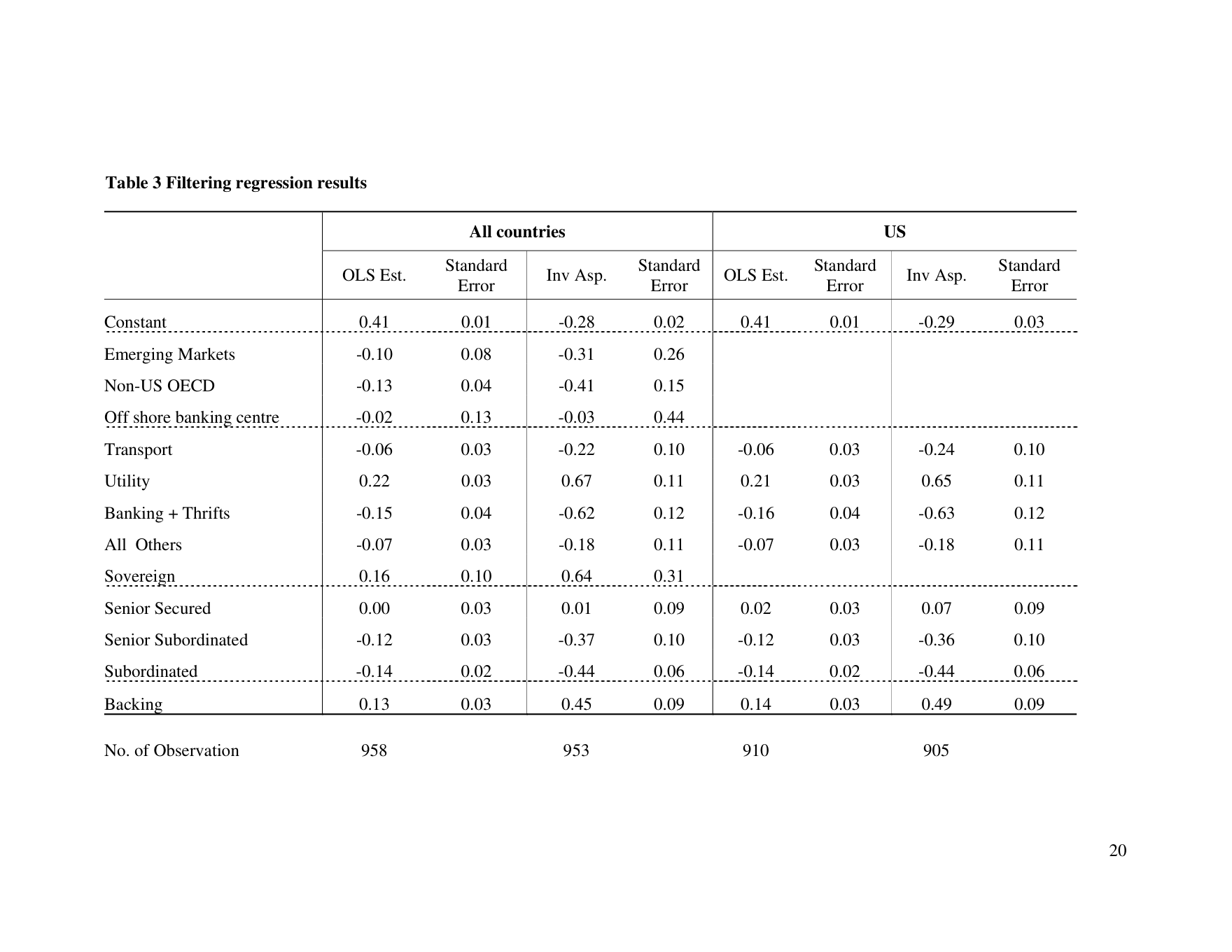
The results of our OLS filter regressions appear in columns 1 and 3 in Table 3. Results are provided for the entire data set and for the observations corresponding to US-domiciled obligors.
Since the dummy variables are demeaned, the constant equals the unconditional mean recovery rate. The constant for all obligors and for the US data are both 0.41. The domicile of the issuer plays a significant role in that recovery rates for non-US OECD issuers are 13% lower than in the US while the standard error is 4%.
The sector of the issuer is clearly important in that public utilities have an average recovery rate 22% higher than the reference type (of industrials) while banking and thrifts have an average recovery rate 15% lower. One might note that these differences have the same signs but are lower than the corresponding differences of 30% and 15-18% shown in Table 2. This illustrates the benefits of employing a multivariate regression that reveals the effects of particular variables while holding other factors constant.
Seniority and backing dummies all have parameter with intuitively reasonable signs and magnitudes. Again, the differences between the seniority effects appearing in Table 3 are smaller than those in Table 1.
3.3 Inverse Gaussian regressions
A complication not so far mentioned is the fact that recovery rates generally lie between zero and unity. (All are positive while a very few observations in the
* dataset (5) exceed unity.) However, the fitted recovery rates Ri will not necessarily satisfy this constraint. The solution we adopt is to transform the recovery rates using a function that maps the unit interval to the real line, run the regressions, form fitted values and invert the function. A convenient function to use is the inverse of the standard Gaussian distribution function.
Columns 2 and 4 of Table 3 show the parameter estimates for the inverse Gaussian recovery rate regressions. The parameter estimates have the same signs as the OLS coefficients and the magnitudes of the standard errors as a ratio to the parameter values are comparable to those of the OLS model suggesting they are estimated with a similar degree of statistical precision. However, the parameter space is different for the inverse Gaussian regressions so one cannot immediately interpret the regression coefficients in terms of percentage recovery rates as one can with the OLS regressions.
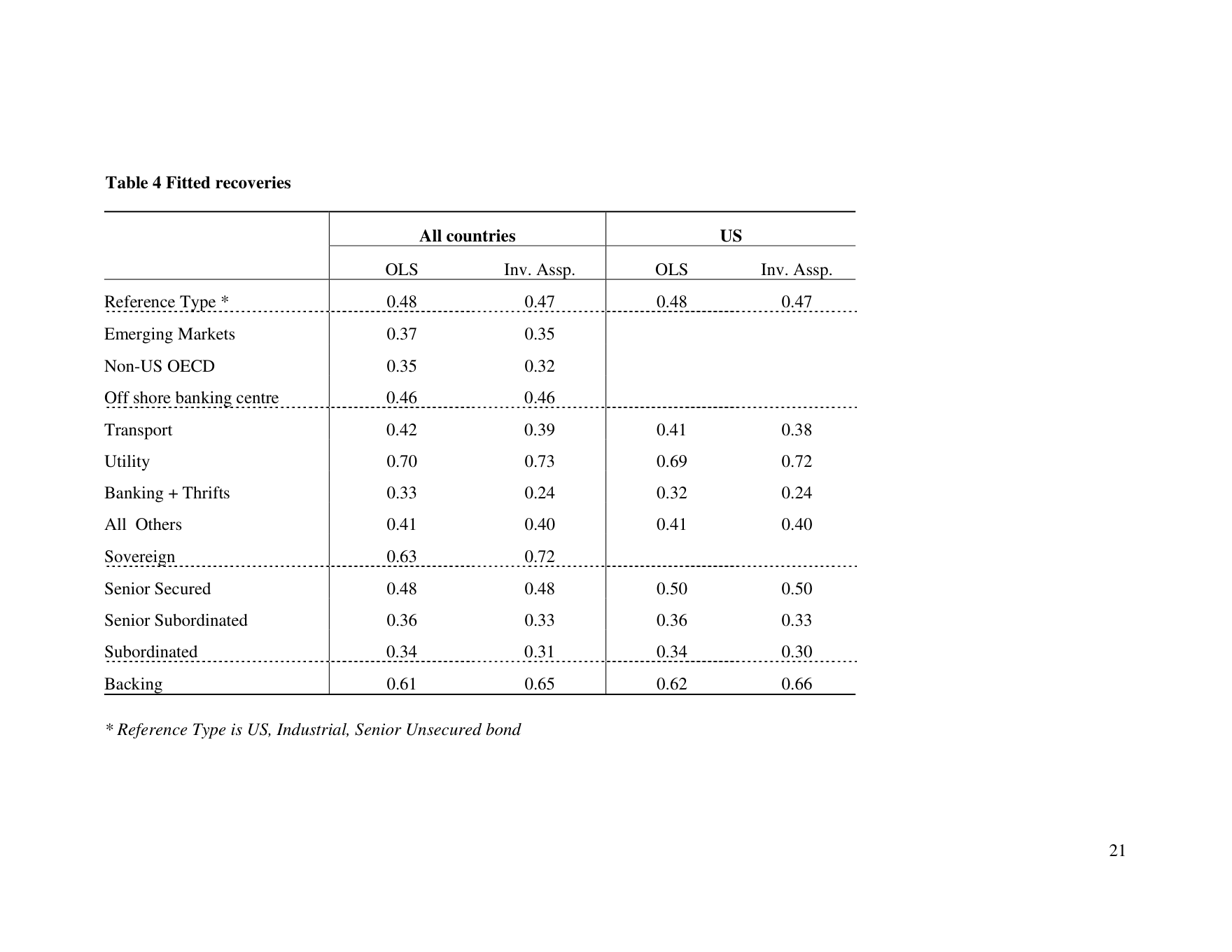
To provide reassurance that the inverse Gaussian transformation does not change the estimated impact of regressors on recovery rates despite the change of parameter space, in Table 4, we show fitted recovery rates for specific issue types. These are calculated by (a) setting εi to zero, (b) calculating the X 'βˆ for a vector of regressors corresponding to a reference type, and (c) varying individual regressors one by one, holding the others constant. As may be seen, the fitted recovery rates are very similar to those obtained using the OLS approach. The advantage of following this approach is that the fitted recovery rates for any εi are always in the unit interval.
4 Default and Recovery Rate Correlation
4.1 Default and recovery rates
Having filtered the recoveries data as described above, we calculate average recovery rates for each quarter in the period 1971 Q1 to 1999 Q4 for US data only. We also calculate default rates for each of these quarters by taking the number of bonds rated by Moody’s at the start of the quarter that defaulted before the end of the quarter and dividing this by the total number of bonds rated by Moody’s at the start of the quarter. Any bonds that are withdrawn during the quarter are left out of both numerator and denominator.[2] From Table 3 we can see that the regression results are dominated with the US data. Furthermore, it would be beneficial to focus only on the US data because the different economic cycle in different countries might contribute to extra volatility of the recovery and default rates.
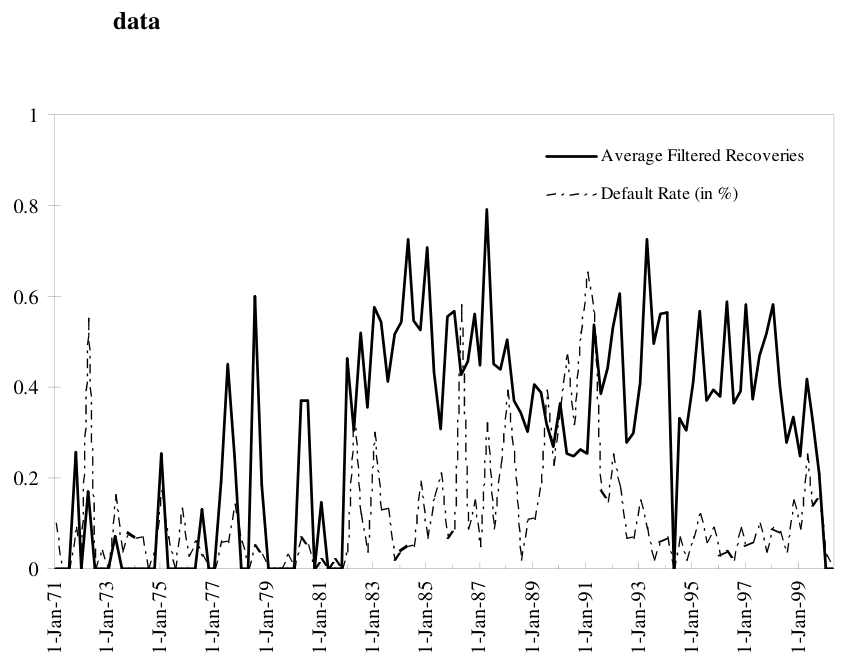
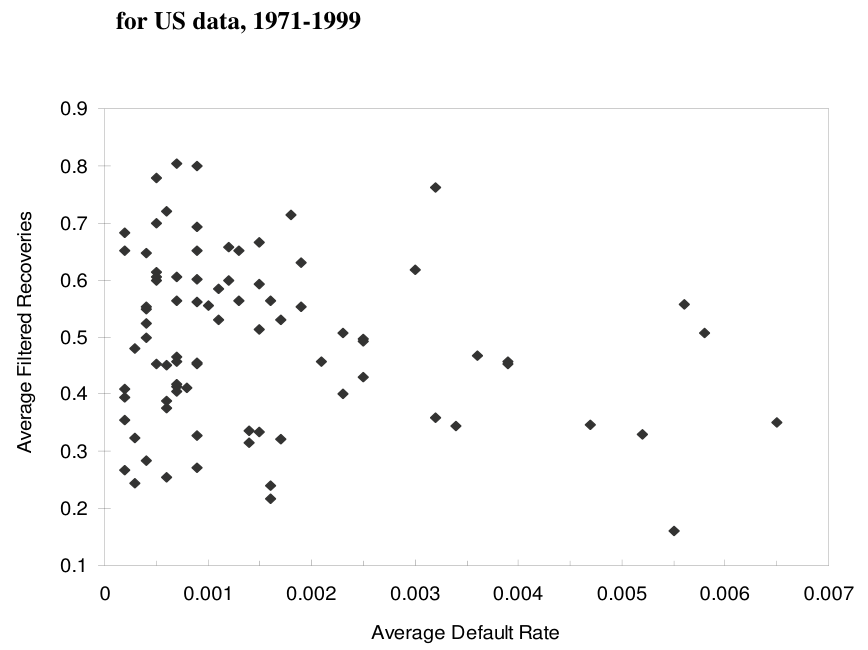
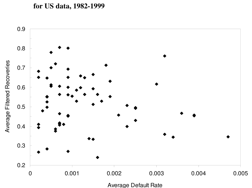
Figure 2 shows time series plots of quarterly average filtered recoveries and default rates over our sample period. There is clear evidence of negative correlations between the two series, especially after 1982. Figures 3 and 4 show scatter plots of the filtered quarterly average recoveries for the periods 1971 Q1-1999 Q4 and 1982 Q1-1999 Q4 respectively. The outlier in the former plot is the 1971 Q2, in which many defaults occurred. Both scatter plots suggest negative correlation.
However, an additional feature of the data that is apparent from the scatter plots is the fact that if one considers only observations for which the default rate exceeds some amount like 5 or 7.5 basis points, the negative dependence appear to be intensified. This is interesting because observations with large default rates are likely to be those that contribute to the tail of the total credit loss distribution and hence matter for VaR calculations and the determination of appropriate capital.
4.2 Correlations
Table 5 reports correlations between quarterly average recovery rates and quarterly default rates under several different assumptions. The standard errors of the correlations are reported in parentheses. The first row represents correlations for unfiltered recovery rates. While the correlations are clearly negative, their absolute magnitudes are less than those in the second and third rows which are based on filtered data using the OLS or inverse Gaussian regression approaches, respectively. Also apparent from these tables is the fact that the correlations using unfiltered data are, broadly speaking, little changed when one drops observations with default rates smaller than 0.05% or 0.075%. However, when the recoveries are filtered, the change become more obvious. These further support our assumption that extra volatility resulting from the fact that Moody’s rated obligators evolve over time plays down the correlation between recovery and default rates.
5 Non-Parametric Estimates of Credit Loss Distributions
5.1 Kernel estimates of loss distributions
To investigate the effect of the dependency between default and recovery rates on portfolio credit risk models or pricing risk models, we calculate risk measures of credit losses, in particular, VaRs, with actual data and with data generated by randomly pairing up default rates and recovery rates from different periods. Through the later procedure, we are able to remove the dependency between the two.
Let Lt be the total credit loss of a portfolio with equal dollar amounts in each of the bonds rated by Moody’s at time t, then Lt = Dt (1− Rt ) (5.1) where Dt and Rt is the default rate and recovery rate at time t. Therefore, our actual series for credit loss contains 85 observations for the period of 1971 Q1 - 1999 Q4 and 71 for 1982 Q1 – 1999Q4.
The density of the loss function f(L), is then estimated using the following kernel estimator:
L − L 1 ⎛ t ⎞ f (L) = ∑ K⎜ ⎟ (5.2) nh ⎝ h ⎠
where h is the width of the interval, n is the number of observations, and the kernel, K, we use here is the standard normal density function: ⎛ ⎞ ⎛ Lt − L ⎞ −[1]/[2] ⎜ 1 ⎛ Lt − L ⎞ ⎟ K⎜ ⎟ = (2π) exp − ⎜ ⎟ (5.3) ⎜ ⎟ h 2 h ⎝ ⎠ ⎝ ⎝ ⎠ ⎠
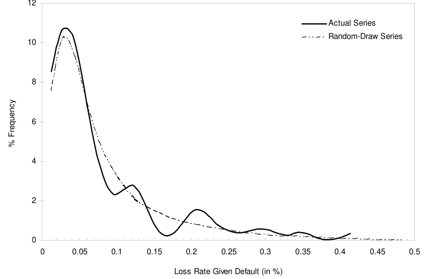
Figure 5 shows the density of total credit losses (i) for the post-1982 US data and (ii) for random draw data. The latter data is created by randomly pairing up quarterly recovery and default rate observations and then calculating total credit losses as defined above. We form a dataset of 100x85 observations of randomly generated total credit losses and then estimate the kernel density shown in Figure 5. The density estimated from actual data appears somewhat more peaked and hence fattailed than the random draw data density.
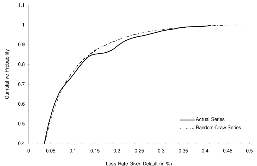
This impression is reinforced when one examines the corresponding cumulative distribution estimates shown in Figure 6. The fat-tailed nature of the distributions is obvious in between in the probability range 0.8 and 0.95. It is hard to tell from the kernel estimates, however, whether the fat-tailed behavior persists further out in the tails. To assess this, it is more appropriate to use a non-parametric technique designed for estimation of tails, which is what we do in the next section.
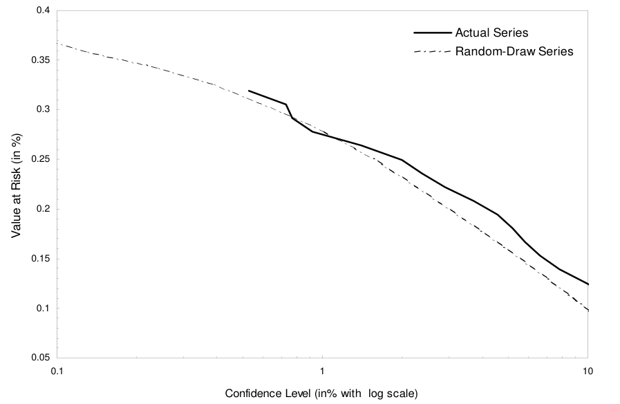
Figure 7 shows VaRs for the “portfolio” for which we calculate credit losses. To understand the results, it is important to recall that the portfolio consists of an equalweight investment in all the bonds rated by Moody’s in successive quarters. Since we employ quarterly data, the VaRs are effectively calculated over a one-quarter horizon. If one used such a holding period in a calculation of capital for a financial institution, one would be assuming that the financial institution holding the portfolio could replenish its capital each quarter.
The VaRs in Figure 7 are shown in percent of the portfolio value on the vertical axis. The range of VaRs is from 0.1% to 0.4%. This is much lower than the typical VaRs one might expect for a bank loan portfolio. Kiesel, Perraudin and Taylor (2001) show that default-mode VaRs (i.e., VaRs based only on realized losses rather than deterioration in credit quality short of default) with a 1% confidence level are around 3.4% for an average US bank portfolio and 1.6% for a high quality bank portfolio. The Figure 7 VaRs are smaller (i) because Moody’s rated bonds have a higher average rating than typical bank loan portfolios and (ii) because of the assumption of a quarterly holding period.
The VaRs shown in Figure 7, consistent with the cumulative distribution plots in Figure 6, suggest that percentage VaRs are higher for the actual data than for the random draw data for confidence levels in the range 1% to 10%. However, for higher confidence levels, it is not clear whether the actual data or random draw data VaRs are larger. Again, to answer the question, we need to employ Extreme Value Theory techniques.
5.2 Extreme Value Theory estimates
Extreme Value Theory (EVT) offers a range of techniques for estimating statistics of the tails of distributions. The main advantage of EVT is that, relying on limiting results of order statistics, it does not require that one assume particular distributions for the underlying data. For a wide class of fat-tailed distributions commonly encountered in finance, Extreme Value Theory results imply that the tail behaviour of the distribution, denoted F(x), is asymptotically given by:
−α 1− F(x) ≡ F (x) ≈ x Q(x)
for a parameter α>0 and a slow-moving function Q(x). 1/α is referred to as the tail index. In applications, Q(x) is generally taken to be constant so that estimation of the tail reduces to one of estimating α.
A variety of techniques have been proposed for the estimation of α. The simplest of
−α these is the Hill estimator. If F (x) = Cx for 0<u<x and C=uα (i.e., the
complementary distribution is approximated with the Pareto distribution) then the Maximum Likelihood estimator of α is just
−1 n ⎛ 1 ⎞ ˆ α=⎜ ∑log X n− j+:1n −logu⎟ n j=1 ⎝ ⎠
Here, Xn-j+1:n denotes the n-j+1 order statistic from a sample of n observations.
The problem with the Hill estimator is that one must select a threshold u beyond which one assumes that the distribution is accurately approximated by the Pareto distribution. Estimates of α often vary significantly depending on one’s choice of u.
Recently, Huisman, Koedijk, Kool and Palm (2001) have proposed a regression estimator for α based on the Hill estimator. This circumvents the problem of selecting u by calculating Hill estimates for a range of different values of u and taking the intercept of the regression (i.e., the “estimate” corresponding to “a zero value of u”) as the estimate of α. This approach while intuitively sensible can be justified statistically as a way of extracting information from a number of different estimators. The regression is complicated by the fact that the estimates for different values of u are correlated. Huisman, Koedijk, Kool and Palm (2001) employ Weighted Least Squares and show how one may calculate standard errors for the resulting α estimate.
Given an estimate αˆ , one may calculate an estimate of the VaR for total credit losses L with confidence level p as:
−1 ˆ α(k,n) n ⎛ ⎞ VaRp = ⎜ 1(− p)⎟ Ln−k:n − L k ⎝ ⎠
Here, n is the sample size, k is an integer less than n and L is the sample mean. Given the standard error of αˆ , one may calculate the standard error of the VaR using the delta method.
Table 8 contains estimates of the α parameter for different samples. The random draw estimates are obtained by (i) generating 100 samples each with the same number of observations as the corresponding actual sample, (ii) estimating α for each sample and then (iii) averaging the α’s. We follow this approach because we are primarily interested in differences between α estimates. If the relatively small sample size introduces some bias, we would prefer that the bias be both in our estimate using actual data and in the estimate obtained using the generated randomdraw data.
Table 6 contains estimates based (i) on data from Q1 1971, and (ii) on data from Q1
1982. In each case, we estimate α using the actual total credit loss data and the random draw samples. A smaller value of α implies more fat-tailed behaviour. It is clear that the random draw estimates are consistent with less fat tails than the estimates based on the actual data.
Figure 8 shows VaR estimates with 1-standard deviation bands based on the post 1982 data. As one may observe, the VaR estimates for confidence levels below 1% are significantly higher for the actual data than those obtained using the random draw data. This suggests that the tail dependence between recoveries and default rates is sufficiently great to imply statistically larger VaRs than would be the case in the absence of tail dependence.
6 Conclusion
This paper has examined the dependence between recovery rates and default rates using Moody’s historical bond market data. Having filtered the recovery data to allow for variation over time in the pool of borrowers rated by Moody’s, we study simple measures of correlation between aggregate quarterly default and average recovery rates. These suggest that recoveries tend to be low when default rates are high. This provides prima facie evidence that risk measures and capital should be higher than one would conclude from calculations that assume independence of recoveries and default events.
To investigate the issue further, we calculate VaRs using the actual data and data from which we have removed dependence by randomly pairing quarterly recovery and default rate observations from different time periods. The VaRs are calculated using a variety of non-parametric techniques. First, we calculate kernel estimates of total credit loss distributions. Second, we use Extreme Value methods based on recent work by Huisman, Koedijk, Kool and Palm (2001). We conclude that there is evidence of VaRs are greater to a statistically significant degree when confidence levels exceed 1%.
References
Altman, E. I. and V. Kishore (1996) “Almost Everything you Wanted to Know About Recoveries on Defaulted Bonds,” Financial Analysts Journal, November- December, 57-64.
Asarnow, E. and D. Edwards (1995) “Measuring Loss on Default Bond Loans: A 24-year study,” The Journal of Commercial Lending, March, 11-23.
Bhattacharyya, G. K. and R. A. Johnson (1977) Statistical Concepts and Mehtods, John Wiley & Sons, Inc.
Carty, L. and D. Lieberman, (1996) “Defaulted Bank Loan Recoveries,” Moody’s Global Credit Research, Special Report.
Embrechts, P., C. Kluppelberg and T. Mikosch (1997) Modeling Extremal Events, Springer.
Fons, J.S. (1994) “Using Default Rates to Model the Term Structure of Credit Risk,” Financial Analysts Journal, September-October, 25-32.
Frye, J. (2000) “Depressing Recoveries,” Risk, November, 108-11.
Greene, W.H. (1997) Econometric Analysis, 3rd edn. Prentice-Hall.
Gupton, G., Finger, C., and Bhatia, M. (1997). CreditMetrics – Technical Document. Morgan Guaranty Trust Co. http://www.riskmetrics.com/research/techdoc.
Hickman, W.B. (1958) Corporate Bond Quality and Investor Experience, Princeton, New Jersey: Princeton University Press.
Huisman, R., K. Koedijk, C. Kool, and F. Palm, (2001) “Fat Tails in Small Samples,” Journal of Business and Economic Statistics, 19(1), 208-16.
Izvorski, I. (1997) “Recovery Rates and Survival Times for Corporate Bonds,” IMF working paper, WP/97/84.
Jarrow, R.A. and S.M. Turnbull (2000) “The Intersection of Market and Credit Risk,” Journal of Banking and Finance, 24(1-2), 271-99.
Jarrow, R.A., D. Lando and S.M. Turnbull (1997) “A Markov Model for the Term Structure of Credit Spreads,” Review of Financial Studies, 10, 481-523.
Kiesel, R., W. Perraudin and A. Taylor, (2001a) “An Extremes Analysis for Emerging Market Benchmark Bonds,” Birkbeck College mimeo.
Kiesel, R., W. Perraudin and A. Taylor, (2001b) “The Structure of Credit Risk: Spread Volatility and Ratings Transitions,” Bank of England Working Paper.
Kijima,M.and K. Komoribayashi (1998) “A Markov chain model for valuing credit risk derivatives,” Journal of Derivatives, 6(1), 97-108.
Litterman, R, and T. Iben, (1991) “Corporate Bond Valuation and the Term Structure of Credit Spreads,” Journal of Portfolio Management, Spring, 52-64.
Pagan, A. and A. Ullah (1999), Nonparametric Econometrics, Cambridge University Press.
Van de Castle, K., and D. Keisman (1999) “Recovering Your Money: Insights into Losses from Defaults,” Standard & Poor’s report.
Figure 8 VaR for 1982 – 1999 credit loss data using WLS estimation of α
0.8
Actual Series 0.7 Random-Draw Series Actual + 1 s.d. Actual - 1 s.d. 0.6 R.D. + 1 s.d. R.D. - 1 s.d.
0.5
0.4 Value at Risk (in %) 0.3
0.2
0.1
0.10 1.00 10.00
Confidence Level (in %, w ith log scale)
| Study Bank | Senior | Senior | Senior | ||
|---|---|---|---|---|---|
| Subordinated. | |||||
| Loans secured | unsecured | subordinated | |||
| Altman & Kishore | -- | 58 | 48 | 34 | 31 |
| Fons | -- | 65 | 48 | 40 | 30 |
| Carty & Lieberman | 71 | 57 | 46 | -- | 34 |
| Van de Castle & Keisman | 84 | 66 | 49 | 37 | 26 |
| Our data | -- | 53 | 50 | 38 | 33 |
Source: Altman and Kishore (1996), Fons (1994), Carty and Lieberman (1996) and Van de Castle and Keisman (1999)
| Industries | Average | Volatility Numbers | of |
|---|---|---|---|
| Transportation | 38.6% | 27.4% | 72 |
| Industrial | 40.5% | 24.4% | 728 |
| Insurance | 39.8% | 21.4% | 12 |
| Banking | 22.6% | 16.6% | 25 |
| Public Utility | 69.6% | 21.8% | 57 |
| Finance | 45.6% | 31.2% | 11 |
| Thrifts | 25.6% | 26.3% | 20 |
| Securities | 15.4% | 2.0% | 2 |
| Real Estate | 25.7% | 17.2% | 8 |
| Other Non-bank | 24.8% | 15.4% | 15 |
| Sovereign | 56.8% | 27.4% | 8 |
| Regions | Average | Volatility Numbers | of |
| Emerging market | 44.1% | 22.1% | 22 |
| Non-US OECD | 39.3% | 27.2% | 23 |
| Offshore banking ctr. | 46.2% | 25.0% | 3 |
| US | 41.0% | 25.7% | 910 |
Note: Greece and Mexico are counted here as emerging market countries not OECD.
| From 1971 | From 1982 | |||||
|---|---|---|---|---|---|---|
| Truncated | Truncated | Truncated Truncated | ||||
| All | All | |||||
| (>5bp) | (>7.5bp) | (>5bp) (>7.5bp) | ||||
| 84 | 66 | 50 | 71 | 57 | 45 | |
| Unfiltered | -0.14 | -0.23 | -0.20 | -0.21 | -0.25 | -0.23 |
| (0.11) | (0.12) | (0.14) | (0.12) | (0.13) | (0.15) | |
| OLS | -0.19 | -0.28 | -0.29 | -0.22 | -0.30 | -0.30 |
| (0.11) | (0.12) | (0.14) | (0.12) | (0.13) | (0.15) | |
| Inverse | -0.19 | -0.27 | -0.29 | -0.22 | -0.29 | -0.31 |
| Gaussian | (0.11) | (0.12) | (0.14) | (0.12) | (0.13) | (0.15) |
| Sample | Alpha | Mean Threshold | |
|---|---|---|---|
| Actual | 3.053 | 0.081 | 0.124 |
| (1.034) | |||
| Random-Draw | 4.222 | 0.077 | 0.125 |
| (1.430) | |||
| Actual | 2.636 | 0.081 | 0.115 |
| (0.893) | |||
| Random-Draw | 4.766 | 0.075 | 0.108 |
| (1.615) |
Notes
[2] This is the correct procedure under the assumption that ratings withdrawals are not correlated with default events or recoveries.