

1. Introduction
The African Development Bank (AfDB) and the Inter-American Development Bank (IDB) have co-developed proposals to boost the lending capacity of Multilateral Development Banks (MDBs) using Special Drawing Rights (SDRs) to create MDB hybrid capital (see AfDB and IDB (2023)). The proposals (henceforth referred to as ‘the MDB Proposal’) have been presented, by the AfDB and IDB, to the International Monetary Fund (IMF) and to other policy audiences.
Under the MDB Proposal, sovereign holders of SDRs would lend them to MDBs that are prescribed holders of SDRs[1], including the AfDB and the IDB. The bonds would be structured to be consistent with rating agency and accounting definitions of hybrid capital. The creation of the additional capital would allow the AfDB, the IDB and other MDBs to expand their lending without incurring pressure on their ratings.
The proposal bears obvious comparison with the schemes operated by the IMF itself whereby SDR holders may lend their SDRs to two trusts which make loans to poor countries, the Poverty Reduction and Growth Trust (PRGT) or the Resilience and Sustainability Trust (RST). Particularly, the PRGT has a long history of successful operation, lending on a short- and medium-term basis to poor countries in balance of payments need. The RST provides longer-term financing in the IMF’s words: “to contribute to prospective balance of payments stability to enhance economic resilience and sustainability”[2]. As such, its lending, while still aimed at balance of payments relief is comparable to MDB lending.
The approach proposed by AfDB and IDB has been widely discussed in development policy circles. G20 Capital Adequacy Framework Review (2022) mentions the MDB Proposal in discussing innovative financing approaches that could boost MDBs’ capacity to lend. Independent Experts Group (2023) page 13 states: “Mobilizing hybrid capital, including through recycled SDRs, and risk transfers to private and public actors to free up capital would also add significant capacity.”
The AfDB and the IDB have commissioned Risk Control[3] to analyse the proposal, focusing specifically on the credit standing and liquidity status of the hybrid capital instruments. Most countries that hold SDRs do so through their central banks, and some are only willing to consider uses of their SDR holdings that maintain their ‘Reserve Asset Status’ (RAS). In other words, they require that SDRs that are lent be immediately available to the central bank in question in the event of a balance of payments crisis. Key characteristics necessary for RAS are high credit quality and liquidity.
This report analyses the credit quality and liquidity of SDRs used to back MDB hybrid equity to assess whether the proposed hybrid capital instruments could be seen as having RAS. Our conclusion that SDR-based hybrid capital will retain RAS implies that countries will be able to account for these instruments as reserves.
Before performing a quantitative analysis (specifically of credit quality), we describe several important safeguards that reinforce the credit quality of MDB hybrid capital.
1. Risk Management Frameworks – MDBs operate with forward-looking Enterprise Risk Management (ERM) frameworks, comparable to those employed by large commercial banks but calibrated more conservatively in that most major MDBs are aiming to maintain AAA credit ratings.
2. Market discipline – MDBs are regular issuers in international bond markets and are subject to the market discipline provided by investors and credit ratings agencies.
3. Preferred Creditor Treatment (PCT) – Key to assessing the riskiness of multilateral organisation portfolios is the de facto seniority that they enjoy in lending to sovereigns referred to as PCT. The analysis in Section 4.3 of this study shows that the credit performance of the portfolios in question would be different if the institutions did not benefit from PCT (for example, because the portfolios were held by private sector organisations).
Turning to quantitative analysis, we analyse the balance sheets (most notably, the credit exposures) of two major regional MDBs, the AfDB and IDB. For each of these institutions, we use a multiperiod Credit Portfolio Model (CPM) to calculate the probability, over different horizons, that issues of hybrid capital would become loss absorbing.[4]
The liquidity mechanism proposed by the AfDB for hybrid capital aims to mimic the arrangements already in use in the PRGT. We describe how this mechanism has performed in recent years. Since it seems to have behaved robustly, we conclude that the proposed liquidity arrangements, if they can be implemented in practice, are consistent with RAS.
The key points that emerge from our analysis are:
1. The credit quality of SDR-based hybrid capital is extremely high. Using parameters (PDs and LGDs) adjusted for PCT within a CPM, the probability that the hybrid capital instruments become loss absorbing is negligibly low for both AfDB and IDB portfolios. Note that when parameters are used that are not adjusted for PCT (i.e., in line with parameters one could use for an Emerging Market (EM) sovereign portfolio of a private sector investor), loss rates are high. So, PCT is a key aspect.
2. On pricing, we model payoffs and loss-absorption related losses on hybrid capital again using a CPM but, in this case, with risk adjusted distributions. The actuarially fair spreads that we infer are very narrow (being no more than a few basis points). This is important because it implies that, if MDBs are willing to pay a reasonable premium over and above this amount, a case could be made to central bank reserve managers that investing in hybrid capital constitutes a valuable investment opportunity.
3. On liquidity, the basic mechanisms for liquidity proposed by the AfDB would be the same for hybrid capital as those employed for the PRGT and RST.
4. On development leverage, the use of SDRs as contributions to hybrid equity is highly efficient, generating a high volume of development finance. By way of contrast, the PRGT or RST require the provision of ‘equity capital’ in the form of donations to the reserve account to achieve a development leverage of unity. One the other hand, one SDR devoted to hybrid capital, can generate higher MDB lending of 3 to 4 deending on the degree of conservatism with which the MDB manages its balance sheet. The leveraging capacity is based on the amount of risk capital and the volume of liquidity that MDBs like AfDB or IDB have to set aside to generate additional loans, assuming a risk profile similar to those of their current balance sheets.
The document is organised as follows. Section 2 discusses the reserve asset eligibility of an SDR provided as hybrid capital to the AfDB or IDB. Section 3 discusses qualitative factors that affect the credit quality of SDRs used to back hybrid capital. Section 4 assesses the credit risk of hybrid capital notionally issued by two MDBs, AfDB and IDB, through (i) presentation of descriptive statistics and (ii) formal simulation exercises with a multiperiod Credit Portfolio Model (CPM). Section 5 presents the analysis for pricing the hybrid capital. Section 6 discusses the liquidity arrangements envisaged by the MDB Proposal. Section 7 concludes.
2. Reserve Asset Status of Hybrid Capital
2.1 Background on Reserve Asset Status
The concepts and methodological standards that define what constitutes a ‘reserve asset’ for the purpose of balance of payments has evolved historically. The main reference work is the IMF’s “Balance of Payments and International Investment Position Manual, Sixth Edition (BPM6)”, published in 2009. The first edition (BPM1) was released in 1948, and the seventh edition (BPM7) is scheduled for issuance in 2025. This version will incorporate updated guidance, such as the September 2022 document “Standardized Statistical Definition of Net International Reserves”. In parallel, the United Nations is working on revising the “System of National Accounts,” (SNA (2008)), and there are close conceptual links between the two manuals.[5]
In 2013, the IMF produced the “International Reserves and Foreign Currency Liquidity (IRFCL), Guidelines for a data template”. This goes into the practicalities of how to report reserve asset instruments and PRGT loans. It starts by repeating the general definition of reserve assets, as per BPM6, paragraph 6.64:
“Reserve assets are those external assets that are readily available to and controlled by monetary authorities for meeting balance of payments financing needs, for intervention in exchange markets to affect the currency exchange rate, and for other related purposes (such as maintaining confidence in the currency and the economy, and serving as a basis for foreign borrowing).”
The paragraph provides additional details including “Reserve assets must be foreign currency assets and assets that actually exist. Potential assets are excluded. Underlying the concept of reserve assets are the notions of “control,” and “availability for use,” by the monetary authorities.”
The term “external assets” underlies the concept of international reserves, and BPM6 makes a distinction between claims on resident and non-residents. The claims on multilateral institutions would qualify for claim on a ‘non-resident’, in a similar way that the IMF-administered trusts (PRGT and RST) are also non-resident.
The term “monetary authorities” is defined in BPM6 and refers to central banks. However, assets not held by such institution would not necessarily be disqualified from being ‘reserve assets.’ Some SDR lenders to the PRGT are not central banks, for example: Government of Australia, Government of Canada, Government of Germany, Government of Japan, Government of Norway, Government of the United Kingdom. BPM6, paragraph 6.66 states “In economies in which extensive reserve assets are held outside of the central bank, supplementary information should be provided on the institutional sector of holdings of those reserve assets.”
The term “controlled by” is caveated in a footnote of BPM6, paragraph 6.64, which states that “Monetary authorities may sometimes employ fund managers to manage reserve assets. In such arrangements, the fund managers are acting as agents and are paid a fee for their services.” A mandated intermediary, acting as agent, is not incompatible with the reserve asset concept. To a certain extent, the trust structure itself in PRGT and RST can be seen as being such intermediary, especially with the PRGT GLA (General Loan Account) where countries do not have bilateral relationships with the end borrowers). In the old structure PRGF-ESF, the loans were bilateral but the creation of the GLA has changed the working approach and efficiency of the PRGT operation. The other notion of control concerning ownership is also satisfied for the PRGT, RST and Hybrid Capital of the MDB Proposal.
On the availability for use, BPM6 stipulates that two conditions must be met: liquidity (paragraph 6.69) and quality (paragraph 6.70)
• “Reserve assets must be readily available in the most unconditional form. A reserve asset is liquid in that the asset can be bought, sold, and liquidated for foreign currency (cash) with minimum cost and time, and without unduly affecting the value of the asset. (No time limit is provided, but to qualify as reserves, an asset should be available in a very short period of time given the speed at which experience suggests a foreign exchange need can arise in adverse circumstances)”.[6]
• “To be readily available to the authorities to meet balance of payments financing needs and other related purposes under adverse circumstances, reserve assets generally should be of high quality.”
At the intersection of control and availability issues is encumbrance. BPM6, paragraph 6.75 has a further clarification on this by stating: “An existing asset that is committed for a future use but not encumbered can be included provided that the asset is readily available to meet a balance of payments financing need (and other related purposes stated in paragraph 6.64). An asset should not be denied as a reserve asset simply because the use to which the asset is to be put is a foreseeable one. However, when an asset is not readily available —such as an asset whose use is blocked— the asset should not be counted as reserve assets.”
The term ‘high quality’ is not defined in BPM6, and quality issues of reserve assets are not further discussed in BPM6. It, thus, comes as no surprise that according to the IMF, the term “readily available” has been variously interpreted by countries. And this is why the IRFCL Guidelines are useful, as they add further clarification as to what was intended. In the context of securities, paragraph 89 mentions: “To be readily available to the authorities to meet balance of payments financing and other needs under adverse circumstances, reserve assets generally should be of high quality (investment grade) {Footnote: Information available from rating agencies can be supplemented by other criteria (including the creditworthiness of the counterparty) to determine the quality of the securities.} If reserve assets include securities below investment grade, this must be indicated in country notes accompanying the data.”
It is clear from the above that the use of regular risk assessment using credit models can provide an acceptable demonstration of the requisite credit quality of a reserve asset.
In terms of reporting, Appendix 8 of the IRFCL Guidelines concerns the statistical treatment of lending to the IMF, lending to IMF managed trusts, and SDRs. Section A8.12 stipulates: “Lending to IMF managed trust accounts, such as the PRGT, if readily available to meet a balance of payments financing need, should be included in official reserve assets, in item I.A.5 of the Reserves Data Template (other reserve assets). These claims are not classified in item I.A.2, RPF, because claims on IMF managed trusts are not claims on the IMF General Resources Account. Lending to IMF managed trusts that is not readily available to meet a balance of payments financing need does not qualify as an official reserve asset and should not be reported in the Reserves Data Template.”
From the above, there is an implicit recognition that lending to PRGT is of ‘high quality’, and that any commitment to PRGT with an encashment clause would easily qualify for the ‘liquid’ element. Nevertheless, there is no mention that a commitment without an encashment clause would be disqualified from being reported to the IMF in item “I.A.5. Other Reserve Assets”.
The remaining sections of this document analyse the credit quality and liquidity of hybrid capital. The creation of such hybrid capital entails the loan of SDR holdings by IMF Member Countries (MC). In most cases, SDRs holders are IMF MC central banks, and these commonly (although not invariably) require that lent SDRs preserve their reserve asset status, i.e., that they be accessible to the lender if it experiences a Balance of Payments (BoP) crisis.
As described in AfDB and IDB (2023), MDB hybrid equity consists of perpetual (but redeemable by the MDB) loans to MDBs by SDR-holders. The loans have loss-absorbing properties in that: (i) coupon payments can be cancelled in some circumstances and (ii) principal written down in case a call is made on the callable capital of the MDB.
2.2 Nature of the hybrid capital
2.2.1 Terms of the hybrid capital
It is important to be clear about the payment structure, maturity, loss absorption and subordination features of the proposed hybrid capital.
The instruments would pay the SDR floating interest rate plus a fixed spread. The hybrid instruments would have a perpetual maturity, with the issuer having a discretionary right to redeem the instrument at par “after a ‘non-call’ period of 10 years after issuance and on agreed subsequent dates after that (for instance, every year after the first call date, or every 5 years etc.), provided that a financial trigger event has not occurred” (see AfDB and IDB (2023).
The fact that the instrument is perpetual should not in itself be viewed as a negative feature. RST loans are long dated and can last for up to 30.5 years and with a grace period of 10 years. The financial risk between a perpetual and a 30-year maturity instrument with a 10-year grace period may be considered minimal, as can be seen for instance by the fact that 30 year is often the proxy for perpetual maturities anyway.
More fundamentally, and as discussed earlier, BPM6 does not require reserve assets to have a finite maturity (equity claims can be accepted). What matters is the availability for use and its liquidity (in other words, one does not rely on the maturity of an asset to ensure liquidity, especially if such asset is long dated).In this regard, the RST loans in 30-year format are no more liquid than the perpetual callable hybrids that the AfDB could issue.
2.2.2 Loss absorption and coupon cancellation
While the proposed hybrid instrument does incorporate some loss absorption features so as to meet accounting and rating agency criteria, it can be argued that the economic risk profile of the instrument remains extremely strong (reflected in its expected investment grade rating).
• The instrument would have a mandatory coupon cancellation upon breach of the capital trigger discussed earlier (excluding any support from shareholders or risk management by the bank itself), and, therefore, can be considered as extremely remote. The cancellation of coupon payments would not, on its own, materially strengthen the capitalisation of the MDB.
• The MDB also has a fiduciary duty to act in the best interest of all its stakeholders. The principal loss absorption at the point of a call on callable capital represents an extremely remote scenario, at which the MDB, having exhausted all other capital raising options, is no longer able to finance itself.
By the time this happened, the MDB would have long since broken its rating and CAR targets and faced market discipline in the form of higher funding costs.
2.2.3 Subordination
The hybrid instrument ranks senior to an MDB’s paid-in equity, and generally benefits from the MDB’s standalone credit strength, driven by its strong capital and liquidity buffers, its diversified portfolio, strong governance, and risk management, as well as its preferred creditor status.
2.3 Liquidity aspects
To ensure the liquidity of PRGT loans, the IMF has implemented encashment and transferability mechanisms. Specifically, “loan claims on the PRGT may be transferred among IMF members, to the central bank or other fiscal agency of a member, or to a prescribed SDR holder. Agreements may contain provisions aimed at further enhancing the liquidity claims on the PRGT […]. Lenders may participate in a voluntary encashment regime in which they have the right to seek early repayment of outstanding claims on the PRGT in case of balance of payments needs and to authorize drawings by the trustee to fund early repayment requests by other participating creditors to any of the loan accounts of the PRGT. Early repayment is subject to the availability of resources under borrowing agreements of other participating creditors.” (See IMF (2018).)
The RST is structured to resemble the PRGT in that SDRs lent to its LA (Loan Account) or DA (Deposit Account) would have the characteristics of reserve assets while RA (Reserve Account) contributions would not. The proposal for creating the RST states: “Liquidity of contributors’ claims on the LA related to outstanding RST loans would be ensured by an encashment regime stipulated in the RST instrument and incorporated into the loan agreements (all LA contributors would have to allow for encashment drawings), where contributors commit to provide access to their borrowing agreements for drawings in the event another contributor experiences a BoP need and requests early repayment its loan claim. Staff would seek to manage the level of undrawn commitments under borrowing agreements in a manner that preserves a buffer for possible encashment requests, parallel to the practice in the PRGT. A lender encashing its RST loan resources would commit to again finance calls for drawings under its loan agreement once it no longer has a BoP need. The encashment regime would require a sufficiently large pool of economically strong lenders.”[7] (see IMF (2022b))
The MDB Proposal for hybrid equity suggests adopting liquidity features resembling those of the PRGT/RST. These would allow SDR lenders to redeem all or a portion of their loan in case they experience BoP issues. It would accomplish this through an encashment regime comprising:
• An encashment clause that SDR lenders could request.
• Temporary transfer of exposures among contributors.
To support encashment, as in the PRGT/RST, the MDB Proposal would ask SDR lenders to provide an unfunded contribution of 20% of their SDR loan. Again, as in the PRGT/RST, the participation of a minimum number of SDR lenders with an extremely strong credit profile would be required. These countries would provide the key element in ensuring the liquidity of the pool. SDR lenders experiencing BoP issues would be permitted to draw down from the unfunded liquidity pool.
Inspection of the patchwork of bilateral agreements through which countries have lent SDRs to the PRGT reveals that the picture of what SDR lenders require to retain reserve asset status is quite varied.
3. Qualitative Risk Factors
3.1 Risk factors
Before we proceed to direct quantification of the credit risk of hybrid capital instruments, we examine qualitative factors that affect the nature of their risks. These factors are hard to capture in a formal model but no less important for this fact.
The three qualitative risk factors on which we focus are:
1. Risk Management Frameworks
2. Market discipline
3. PCT intensity
In the following subsections, we discuss these issues in turn and examine their significance for understanding the credit quality of the hybrid capital usage of SDRs.
3.2 Risk management frameworks
In this subsection, we compare the Risk Management Frameworks employed by MDBs and IMF-sponsored funds and how these may affect the relative credit risk of MDB hybrid capital versus loans to IMF-sponsored trusts.
Institutions’ capital adequacy[8] and liquidity frameworks are affected by their organizational purposes and priorities. MDBs focus on financing development by raising funding in international bond markets and deploying it in development-related loans and equity investments.[9] MDBs aim to maintain a high rating through prudent risk management so that their own funding cost is low. This permits them to lend at low rates to borrower countries which often themselves have low credit status. The approach is possible only because of MDBs’ PCT, the de facto seniority that borrower countries accord certain institutions, including MDBs. MDBs, although they are unregulated, follow the approach of regulated financial firms worldwide (including banks, insurers, and securities firms) of adopting Enterprise Risk Management (ERM) methods. These methods commonly include a Capital Adequacy Framework (CAF) (revolving around quantification of Economic Capital and its comparison with Capital Resources) and a Risk Appetite Framework (RAF) (which involves the systematic adoption of limits on various categories of exposure).
In this, MDBs follow the advice of influential regulatory institutions. For example, the Financial Stability Board argues that: “Establishing an effective RAF helps to reinforce a strong risk culture at financial institutions, which in turn is critical to sound risk management. A sound risk culture will provide an environment that is conducive to ensuring that emerging risks that will have material impact on an institution, and any risk-taking activities beyond the institution’s risk appetite, are recognised, escalated, and addressed in a timely manner." (See FSB (2013).) MDBs also commonly employ long-term financial sustainability frameworks which are used to monitor the Bank’s key internal ratios and those employed by credit rating agencies, and to apply financial levers, including reduced risk taking activities, to maintain these ratios commensurate with meeting AAA standards..
Generic MDB Principal Metric: For most, the Capital Utilization Rate (CUR) = Total required capital/Total available capital
Hard Ceiling: CUR < 100% with buffers and triggers at lower thresholds
Policy Target: To preserve the AAA rating while minimizing the probability of having to draw on callable capital.
Source: G20 CAF Review (2022).
AfDB Principal Metric: Risk Capital Utilization Rate (RCUR)
• Core Risks RCUR < 100%
• Non-Sovereign RCUR < 45%
• Concentration Limits expressed in RCUR. For example, the sum of capital consumption of individual exposures to a particular country must be less than a percentage of total RCUR. Also, the total exposure to individual counterparties must be less than specified percentages of RCUR.
• The AfDB RAS also defines the target credit quality of the core risks, i.e., the Weighted Average Risk Rating (WARR) of the combined sovereign and nonsovereign portfolio, of the sovereign portfolio, of the non-sovereign portfolio, and of the equity portfolio.
Policy Target: To protect the AAA rating. Like other MDBs, the AfDB’s development lending model relies on its ability to mobilize adequate long-term funding from the international capital markets at the lowest cost. To ensure continuous access to this funding, the AfDB’s over-arching enterprise risk management objective is to protect its AAA credit rating under all reasonably probable stress scenarios.
Source: AfDB’s RAS 2022.
IDB Principal Metric: Capital Coverage Ratio (CCR), constructed as the ratio of Adjusted Equity to Base Capital Requirements, or the inverse of the AfDB’s CUR.
Policy Target: To protect the AAA rating. The policy mandate refers to IDB’s long term, foreign currency credit ratings with all major credit rating agencies. The capital buffers are defined “in order to maintain the before mentioned credit rating even in times of stress.”
Source: IDB Capital Adequacy Policy 2014.
The Risk Appetite Statement (RAS) of an MDB is the primary board-level policy document articulating its willingness to assume risk in pursuit of their development mandate. The main content of the RAS is a set of limits or agreed approaches to generating limits. Limits constrain exposure to country, sector, and individual obligor. The limits may be expressed in terms of notional value, Exposure at Default or Economic Capital consumption. The RAS may contain require the institution to maintain a particular agency credit rating or the requirements may be stated elsewhere, in statutes or board-level policy documents.
Commonly, an MDB RAS places a limit on the ratio of capital requirements to capital resources, i.e., the Capital Utilization Rate (CUR).[10] MDBs distinguish two notions of capital resources:
a) Available Capital, a narrow view of risk capital, made from paid-in capital, retained earnings and reserves, with minor adjustments for payment schedules, and
b) A broader notion of capital comprising Available Capital and Callable Capital.
Each MDB has devised its own way of computing capital requirements. Most employ conventional commercial bank risk measurement tools such as Credit Portfolio Models (CPMs) and Value at Risk or Expected Shortfall Market Risk models. Operational risk is commonly measured using regulatory standardized approaches.
To illustrate, in 2014, following market practice, the AfDB migrated its CAF to an “Economic Capital” approach. This change was enabled by the licensing of Credit Portfolio Model (CPM) software that allows the AfDB to assess its capital requirements based on a dynamic Monte-Carlo simulation of potential losses from its balance sheet. Since 2014, the AfDB has used this Economic Capital approach for calculating risk metrics and as the basis for the various risk limits set out in its Risk Appetite Statement.
The Required Capital for AfDB is the Total Capital Consumed (TCC), the numerator in the calculation of the RCUR. TCC represents the amount of the bank’s risk bearing capacity (risk capital) that is required to absorb total potential unexpected losses at a given point in time. TCC is the sum of the risk capital consumption (RCC) for unexpected losses from all sources of risk including the effects of any risk transfer transactions as well as any diversification benefits between individual assets/portfolios and between types of risks.
For Operational Risk, the AfDB continues to apply a standardized approach (the Basel 2 Basic Indicator Approach - BIA) for estimating risk capital consumption for operational risk rather than the Economic Capital methodology used for loans and treasury exposures. Applying the Basel 2 BIA, the RCC for operational risk is 15% of the Bank’s 3-year moving average of annual gross income.
The IDB calculates capital requirements for the different risk types that it faces, i.e., credit, market, and operational risk, and then aggregates these to obtain a total capital requirement allowing for diversification across risk types. Credit Risk is calculated for Sovereign Guaranteed portfolio (SG), Non-Sovereign Guaranteed portfolio (NSG) and Derivative counterparties.
The IDB applies a “sustainability” approach for its SG portfolio. Under this approach, a non-accrual shock is generated at the 10-year confidence level equivalent to a triple-A. The model uses country correlations, adjustments for PCT (which reduce standard PDs), a Loss Given Default based on the IDB’s expectation of full recovery of all overdue interest and principal after the end of a non-accrual event, and a Credit Conversion Factor (CCF) for approved and signed undrawn loan balances.
The level of capital requirements for credit risk in NSG lending is based on a stochastic simulation of individual loans and guarantees, employing a 3-year confidence level equivalent to a triple-A, a correlation matrix based on global, country and industry factors, and transaction-specific PDs and LGDs.
Note that the tools that are deployed by MDBs for the analysis and management of their whole balance-sheet risk are directly relevant and applicable to the risk faced by SDR lenders contributing hybrid capital. At any given moment, the event that would trigger a call on the equity is transparently defined decline in equity value. Conditional on a multi-year lending plan (the size of which is under the control of the bank itself), an MDB’s existing frameworks and reporting arrangements can be redirected to analyse the likelihood of a hybrid equity call. As far as SDR lenders are concerned, the MDB’s policy target of retaining a AAA-rating provides an additional early trigger since a high rating is not consistent with losses on the scale necessary to generate an equity call.
3.3 Market discipline
This subsection examines the role of market discipline in affecting the risk management of MDBs. Most MDBs make regular approaches to the international bond market for funding. This means that their risk profiles are the subject of investigation by investors. To support the funding programs, MDBs commission major Credit Rating Agencies (CRAs) to provide regular appraisals.
Financial regulators have viewed market discipline as very important in enforcing good risk practices. In “Enhancing Bank Transparency” (see BCBS (1998)), the Basel Committee on Banking Supervision discussed in some detail the arguments surrounding the encouragement of market discipline through disclosure. The paper discusses the costs and benefits of disclosure and concludes that an appropriate level of timely disclosure will have benefits for well-run institutions, investors, and depositors, for financial stability more generally, and will help support the effective and efficient operation of the capital markets.
In early 2001, a first consultation document (see BCBS (2001)) on the future Basel II framework, made market discipline the third pillar, in recognition of its potential to reinforce minimum capital standards (Pillar 1) and the supervisory review process (Pillar 2), to promote safety and soundness in banks and financial systems. It states: “Market discipline imposes strong incentives on banks to conduct their business in a safe, sound, and efficient manner. It can also provide a bank with an incentive to maintain a strong capital base as a cushion against potential future losses arising from its risk exposures.” Market discipline was to be supported by an appropriate public disclosure regime, and was to help banks to assess risk, maintain capital and develop and maintain sound risk management system and practices. While the sensitivity of counterparties to market discipline varied, the Committee recognised that “No internationally active bank could, however, expect to insulate itself entirely from the judgements of markets.”
Another form of enforcing market discipline on banks is the use of credit ratings. In Kolaric et al. (2021) shows that, for 154 international financial institutions, between 2004 and 2015, rating downgrades for internal reasons, such as adverse changes in the operating performance or capital structure of banks, are associated with a significant credit default swap spread widening, except for those banks that are perceived as Too-Big-To-Fail (TBTF).
Rating agencies have upped their game and increased their transparency when publishing their credit ratings on MDBs, with one of them publishing an annual comparative compendium: “Supranationals, Special Edition, S&P”. In fact, no MDB (apart, possibly, from the IBRD) would be considered by the market as too big to fail which explains why market participants pay particular attention to their credit ratings. In turn, many MDBs, including the AfDB and IDB, have incorporated the objective of maintaining a triple-A rating directly implement in their risk management policies.
In the case of the PRGT and RST, there is a certain level of disclosure as the IMF publishes every month, the amount outstanding per borrowing countries, but there is no regular quantification by rating agencies of the risks taken by the lenders. And, as the PRGT and RST do not depend on capital markets, they do not need credit ratings. One might even argue that, for the PRGT or the RST to be effective safety valves for countries’ BoP issues, they should not be subject to market discipline.
3.4 Preferred Creditor Treatment
The broader aspect of loan credit performance which affects all the portfolios examined in this report is Preferred Creditor Treatment (PCT). PCT reflects the fact that sovereigns that experience financial distress are not bound by a national insolvency code that enforces equivalent treatment of debtholders with the same contractual seniority. Instead, sovereigns can choose to which of their creditors they will default. In practice, one may observe that sovereigns commonly accord favour terms to certain creditors, in particular multilateral lending institutions, most notably MDBs and the IMF.
A series of past studies has sought to explains the phenomenon of PCT. Fries and Buiter (2002) suggest multilateral lenders receive favourable treatment because they lend at below-market rates. Humphreys (2015) argues that PCT reflects the fact that multilaterals lenders are mutual organisations. Since their borrowers are also shareholders, distressed borrowers provide the multilateral with favourable terms. Levy Yeyati (2009) suggests that institutions like the IMF are accorded PCT because the Fund is willing to lend in crisis periods. Indicators of these MDB characteristics factors (low-rate lender, mutual lender, and countercyclical lender) are collected and analysed by Perraudin and Yang (2017) who suggest that multiple factors may contribute. Cordella and Powell (2022) propose a model in which MDB PCT arises as an equilibrium outcome when MDBs “can commit to lend at the risk-free interest rate and […] credibly limit the amount they lend […]. Atomistic private lenders are not able to coordinate to replicate this contract.”
Second, several studies have attempted to quantify PCT. Most notable among these is Schlegl, Trebesch and Wright (2019) which compares sovereign arrears rates (the ratio of debt in arrears to debt outstanding) for different creditor types using information from the Bank of England-Bank of Canada dataset and find that the IMF and MDBs appear to be the most senior creditors. The arrears ratio on which they focus is hard to relate to standard risk management quantities such as capital or provisions. They also examine LGDs on sovereign restructurings using Paris Club information. These latter are informative about the relative seniority of official
(bilateral) and private creditors but not as regards the seniority of multilateral lenders.
Clear statistical evidence on the magnitude of PCT effects is contained in several Risk Control studies. Perraudin and Yang (2017) calculate the probabilities that African sovereigns will fall into arrears on debt of different types including MDB and IMF loans. Their results suggest that the default rate on IMF loans for African sovereigns is slightly higher than that experienced by the AfDB. More elaborate recent statistical exercises completed by Risk Control for the G20 CAF Panel (see Risk Control (2022)) directly compares PDs for MDB sovereign loans and for private sector debt (through sovereign Foreign Currency (FC) loans or FC bonds). The samples employed are exactly aligned to permit a rigorous comparison by considering years in which countries had borrowed from both sources. These analyses show the very substantial magnitude of PCT for MDBs. Typical PDs are around a third of those experienced by private sector lenders while LGDs for MDBs are between a quarter and an eighth of those obtained by holders of private bonds.
4. Comparative Analysis of Credit Quality
4.1 Leverage analysis of the hybrid capital proposal
This section analyses quantitatively the credit quality of the hybrid capital proposed by AfDB. The calculations draw on the balance sheet data for AfDB and IDB in Appendix 1.
To understand the credit risk of the instruments, one must explain the context of the balance sheet management adopted by MDBs. Specifically, one must grasp what leverage policies the institutions employ.
Recall that the trigger mechanism proposed by the AfDB is for hybrid capital to become loss absorbing if
1. the ratio of Development Related Assets (DRAs) to equity exceeds 5,
2. the ratio of Total Assets (DRAs and Treasury Assets) to equity exceeds 7.5.[11]
Let D represent DRAs and E equity. A loss proportional to development assets of γ× D will reduce both the numerator and denominator. The maximum loss, γ∗, that may be incurred before the trigger is hit may be expressed as: D (1−γ∗) (4.1) E−γ∗ D = 5
5×E/D− 1 γ∗ = (4.2) 5−1
End-2022 AfDB data implies a DRA to equity ratio of D/E= 2.67. This implies γ∗ = 21.9%. Historical MDB data suggests that Loss Given Default (LGD) rates on sovereign loans may be in the region of 10%.[12] So, the trigger of 5 might be thought of as being consistent with a scenario in which (i) the entire development portfolio defaults and (ii) LGDs turn out to be unusually high (more than half greater than usually experienced).
Let the ratio of Treasury assets to DRAs be denoted β. Then, the maximum loss, γ∗∗, that will hit the second trigger proposed by the AfBD is defined as:
D(1+β) (1−γ∗∗) (4.3) E−γ∗∗ D (1+β) = 7.5
7.5×E/D−(1+β) γ∗∗ = (4.4) (7.5−1)(1+β)
For the AfDB 2022 balance sheet, β= 56.0%, which implies γ∗∗ = 12.3%.
If the MDB hybrid capital proposal is accepted and the bank does indeed proceed to boost its equity in this way, it will have to decide what increase in DRAs assets would be advisable. The leverage decisions made will be crucial in determining the credit risk of the new hybrid capital.
If the bank were to boost its DRAs in proportion to the increase in equity, the D/E ratio would remain at the same distance from the trigger as it was before the capital change. Hence, the same portfolio loss of γ∗ = 21.9% would be required before the hybrid capital was called.
The ratio of total assets to equity of (1 + β)D/E would fall unless Treasury assets were also increased. One could expect that a higher volume of Treasury assets would be required to meet the liquidity needs of the larger DRA portfolio but there would likely be economies of scale in the management of liquidity. Hence, a proportionate increased in DRAs and equity would probably move the total assets to equity ratio further from the trigger value of 7.5.
Let us suppose that the AfDB adopts a less conservative policy of increasing DRAs by a somewhat higher proportion than its equity. Let δ denote the ratio of the proportional increase in equity to the proportional increase in DRAs. The level of δ may be chosen so that the loss required to trigger loss absorbance by the hybrid capital equals a target value. Then, if E and D equal the pre-capital increase levels of equity and DRAs, and a 20% loss rate for γ∗ is targeted, one may solve:
5×δ×E/D− 1 (4.5) 0.2 = 5−1
to obtain δ. For the end-2022 AfDB value of E/D, this would imply that the equity rise divided by the target asset increase be 0.96.
The corresponding loss for the 7.5 total-assets-to-equity trigger (if we assume that β remains constant) is:
7.5×0.96×E/D−(1+β) γ∗∗∗ = (4.6) (7.5−1)(1+β)
This implies that γ∗∗∗ = 11.2%.
Below, when we calculate the credit risk of hybrid capital using a quantitative Credit Portfolio Model (CPM), we will draw on the logic just described in that we will consider the probability over different horizons of that losses will exceed 20% on DRA and 11.2% on total assets. It should be clear from the above discussion that credit quality crucially depends on assumptions on how the balance sheet is managed.
The approach to balance sheet management also affects the development finance impact of the hybrid capital investment. One may ask, what is the development leverage of a 1 SDR contribution to the AfDB’s hybrid capital? The impact effect on DRAs from an extra SDR of capital if the policy just described is followed is simply (D/E)/0.96. Hence, the leverage achievable for a holder committing an SDR to the hybrid equity under this policy followed by the AfDB is the current leverage rate of the bank (for which, see the values in Appendix 1) plus 4%, i.e., 278%.
Note that the AfDB’s current leverage ratios (i.e., (1 + β)D/E of ‘Financial Leverage’ when defined with total assets, and D/E or ‘Development Leverage’ when defined with DRAs alone in the numerator) represent key risk metrics for the institution. Like other MDBs, in determining its leverage ratios, the AfDB faces a trade-off between increasing the volume of development finance and ensuring financially sustainability (which gives it access to low-cost funding).
4.2 Credit quality comparisons
In this subsection, we present descriptive statistics that reveal credit quality. For a debt portfolio, credit quality, at an elevated level, is reflected in two key characteristics: Weighted Average Borrower Rating (WABR) and granularity. Table 4.1 provides information on WABRs and granularity of various MDBs, including AfDB and IDB as published by Moody’s for the fiscal year 2020.[13]
EBRD European Bank for Reconstruction and Development B2 16.7 6.7 EIB European Investment Bank Ba1 12.5 5.9 IDB Inter-American Development Bank B3 12.5 5.9 IBRD International Bank for Reconstruction and Development B1 20.0 1.0 IDA International Development Association B2 16.7 1.0 IFC International Finance Corporation B2 20.0 4.3 IsDB Islamic Development Bank B3 25.0 6.3 NIB Nordic Investment Bank Baa2 4.8 5.6 MDB Average B1 15.4 4.5 Note: The source for individual MDBs results is Moody's (2021) and Risk Control for the average. Data relates to end 2020. The measure of granularity employed is the inverse of the Herfindahl-Hirschman Index[14], a common measure of market concentration. This may be thought of as the ‘equivalent number of equal-sized’ exposures.[15] Granularity can be assessed along risk dimensions, such as country risk or industry sector risk.
The nature of MDBs activities implies that the WABR is volatile, changing as the country landscape in the region in question evolves and agencies ratings change for emerging markets. AfDB’s DRA-portfolio WABR has oscillated between B2 and Ba3 since 2006, for example. Many countries represented in the portfolio are not explicitly rated and Moody’s WABR estimates depend on its own private shadow rating of the unrated countries. Similarly, IDB’s WABR fell to B3 in the fiscal year 2020, but was B2 in the previous year that, and Ba3 in 2017.
Comparisons based on a single agency’s ratings may yield unreliable conclusions because of split ratings. For example, Argentina was downgraded by Moody’s to Ca on 3rd April 2020 from Caa2 on 30th August 2019, whereas S&P upgraded Argentina to CCC+ on 7th January 2020 from CC on 30th December 2019. Argentina has been among the top 5 exposures of the IDB Development Portfolio so a WABR calculation using S&P ratings would be materially different.
Figure 4.1 displays ratings distribution for the AfDB and IDB end-2022 development portfolios using Standard & Poor’s (S&P) ratings and employing a shadow rating mapping devised by Risk Control for countries without an official S&P rating, on an updated portfolio. From this we can calculate, a Weighted Average Borrower Rating (WABR), which is provided in Table 4.2. While the WABR difference between AfDB and IDB is about one rating notch (+1 for Moody’s and -1 for the S&P style).
If we now turn to portfolio granularity, the data in Table 4.1 suggest that AfDB has one of the most diverse MDB portfolios with a Country Granularity of 20.0. This reflects the fact that Africa has more countries than other world regions, and that AfDB’s risk management practices allows it to transfer risk to reduce country concentration.[16] On the other hand, IDB has one of the most concentrated portfolios among MDBs with a Country Granularity of 12.5, a reflection that the region covered by IDB has fewer countries to serve, and the development needs are less widespread regionally. We calculate the granularity of AfDB as 21.87 and of IDB as 13.18 for their end-2022 portfolios.
Another indicator of portfolio country concentration risk is that employed by Fitch, which tracks the proportion of the portfolio represented by the 5 largest exposures (“Top 5”). Figure 4.2 shows that, for this measure, the AfDB records 35% and IDB 55% of its portfolio concentrated in the Top 5 countries.
Additionally, we perform a similar credit analysis for AfDB and IDB treasury portfolios (we consider only the bonds). Both treasury portfolios have an average rating of AA+/AA. Figure 4.3 shows the rating distributions of these portfolios. Figure 4.4 shows the 5 countries with the largest exposures in these portfolios.
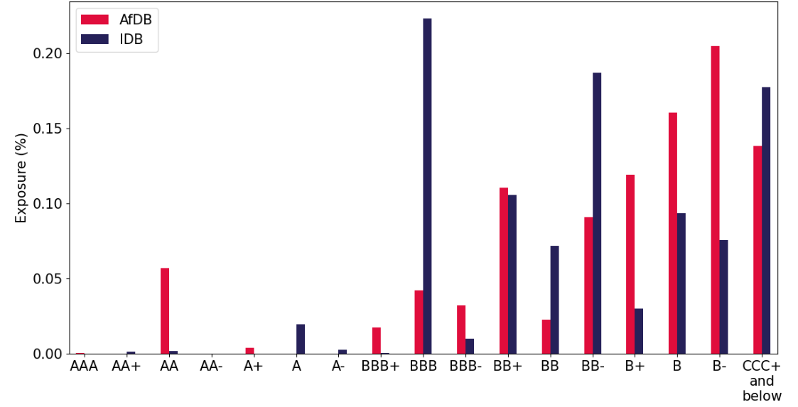
Note: Sources are AfDB, IDB and Risk Control. The data is from the end of 2022 and the exposure amount is based on EAD. We consolidate the ratings below CCC+ in one rating and drop the exposures that are in default.
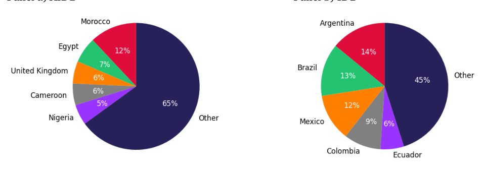
Note: The source is Risk Control calculations based on AfDB and IDB data. DRA figures are based on EAD (including 50% of undisbursed commitments). We consolidate the ratings below CCC+ in one rating and drop the exposures that are in default. For Treasury, we only include bonds. For IDB, the EAD for bonds is assumed to equal the market value. For AfDB, EAD is the Net Notional Amount.
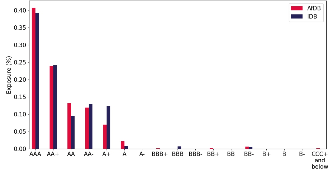
Note: Sources are AfDB, IDB and Risk Control. The data is from the end of 2022 and the exposure amount is based on EAD. We consolidate the ratings below CCC+ in one rating and drop the exposures that are in default.
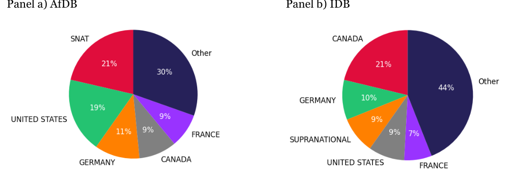
Note: The source is AfDB and IDB. The figures are based on EAD.
| MDB Multilateral Development Bank | Moody’s WABR | Country Risk Granularity | Sector Risk Granularity | ||
|---|---|---|---|---|---|
| AfDB | African Development Bank | B2 | 20.0 | 4.8 | |
| ADB | Asian Development Bank | Ba3 | 11.1 | 5.6 | |
| AIIB | Asian Infrastructure Investment Bank | Ba2 | 10.0 | 2.4 |
| MDB | Multilateral Development Bank | S&P-style |
|---|---|---|
| AfDB | African Development Bank | BB-/B+ |
| IDB | Inter-American Development Bank | BB/BB- |
4.3 Model-based quantitative credit quality comparisons
In Section 4.1, we described a policy that the AfDB could follow is boosting its equity (through issuance of hybrid capital) by slightly less, in proportional terms, than it increases its DRAs. This would have the effect that, post the capital and lending increase, the loss on the DRA portfolio that would trigger the loss absorbing properties of the hybrid capital would equal a prudent value of 20%.
This subsection sets out the methodology we use to assess the relative credit quality of the two portfolios, AfDB’s Development Related Asset (DRA) portfolio and IDB’s Sovereign Obligors (SOs) and Non-sovereign Obligors (NSOs).
The proposed hybrid equity will absorb losses when trigger events occur. The trigger events may be summarised as follows. The trigger kicks in when either:
1. DRA divided by Paid in Capital and reserves exceeds 5, or
2. Total assets divided by Paid in Capital and reserves exceeds 7.5.
To compare credit quality, we calculate, for each of the two MDB (AfDB and IDB) portfolios, the probability that DRAs divided by Paid in Capital and reserves exceeds 5 (because losses exceed 20%).
To calculate the probability that the trigger event occurs, we simulate the ratings of the individual sovereign and non-sovereign loans in each bank’s portfolio forward in time. This provides time series of individual ratings that for SO occasionally dip into (and then re-emerge from) the default or arrears state. For NSOs, default is assumed to be an absorbing state in that, once a default has occurred, no re-emergence from this state is possible.
When an SO remerges from default, we assume that it the par value of exposure to it is the same as that before default. Its rating after emergence is assumed to equal to the rating that it had in the initial portfolio. To achieve these aspects of the re-emergence ratings, the last row of the transition matrix (TM) takes the form:
The table below illustrates an example rating path of a BB-rated SO exposure.
For an NSO exposure, we assume that after default, it is replaced in the portfolio with another exposure in the same country with the same par value and the rating that the NSO had in the initial portfolio. We use a single rating time series to represent a sequence of rated exposures. The last row of the transition matrix will be of the form:
The table below illustrates an example rating path of a BB-rated NSO exposure. We assume that the par value of the exposures remains constant over time and equal to the values initially observed in the portfolio.
After generating the ratings time series for all exposures in the portfolio, we can calculate the time series of cumulative portfolio losses for each Monte Carlo (MC) replication. When an exposure defaults, a provision is calculated by applying an LGD to the par value of the exposure. These provisions are summed over time to obtain simulated cumulative portfolio losses. Additionally, we assume that MDBs earn 0.2% of EAD each period and this is subtracted from the losses.
The LGDs are calibrated to be appropriate for MDB DRA and Treasury SO and NSO exposures, which are presented in Table 4.7.
We used the transition matrices from S&P 2022 annual sovereign and corporate studies with smoothing to ensure monotonicity. For the treasury portfolios, we assumed that there are no rating transitions except defaults. Table 4.8 shows the PDs employed in the analysis. The SO (PCT) probabilities of default shown in the table allow for Preferred Creditor Treatment. Risk Control (2022) shows, with a matched sample of countries and years, that historical PDs for MDB loans are substantially lower than PDs on the sovereign bonds. The scaling factor is 3.6. The SO (PCT) PDs shown in Table 4.8 equal the values of SO (no PCT) scaled by this factor.
For each Monte Carlo (MC) iteration, the time series of portfolio losses and probability of a hybrid capital loss event are calculated as follows.
1. Starting from a current date 0, for each future date t, we calculate the loss due to default and income for each loan i as (4.7) Li,t = EADi × LGDi × Ii,t −EADi × 0.002
Here Ii,t is a binary default indicator equalling 1 in a default event and zero otherwise.
2. The total cumulative loss of the portfolio at time t is calculated as
K (4.8) i=1 Li,t Lt = Lt−1 + ∑ , t= 1,2, . . . … , T, L[0] = 0
3. The MDB hybrid capital starts to absorb losses if the total loss divided by the total EAD exceeds γ∗ = 20%.
4. The probability of a hybrid capital loss at a future date t, denoted PLt, is calculated as:
nt (4.9) PLt = N
Here, nt is the total number of MC iterations in which losses exceed γ∗ = 20% and N is the total number of MC iterations.
We simulate rating time series up to 20 years for each bank’s portfolio using 500,000 iterations and the PLs for the two portfolios are given in the Table 4.9. Panel a) of the table presents results with risk parameters (loan PDs and LGDs) appropriate to private sector lenders such as the international bond market (i.e., without PCT adjustments). Panel b) shows results with parameters appropriate for multilateral institutions such as MDBs that enjoy effective seniority in lending to sovereigns, i.e., with PCT adjustments. Results are presented for the two MDBs (AfDB and IDB).
The main conclusions to draw from Table 4.9 are as follows:
• The contrast between the cases without and with PCT adjustments is very striking. In performing the calculations, we have cumulated losses and allowed for flows of accumulated revenue from lending (20bps each period).[17]
• The probabilities of loss without PCT adjustments are higher for the PCT than for the MDBs.
• When PCT-adjusted parameters are employed, the probability of loss is zero in the sense that, for no iteration is a loss experienced for any institution up to a 20-year horizon.
We perform additional calculations the results of which are shown in Table 4.10 in which we consider the likelihood that hybrid capital loss absorption will be triggered allowing for both DRA and total asset triggers operating together. Again, we suppose that the first trigger ratio for the DRA portfolio operates when losses exceed 20%. We calculate appropriate loss levels for the combined portfolios using the actual Treasury/DRA ratio in the two MDB’s current balance sheets.[18] The assumed loss level for the second trigger ratio is shown in
In Table 4.11, we also provide standard 1-year and 3-year-horizon Value at Risk (VaR) calculations for the three parameters with and without PCT adjustments. All VaR statistics are reported as percentages 0f the portfolio Exposure at Default (EAD).

Note: In this example, the initial rating of the SO is BB. The probability of remaining in default is 0.8, and, if the SO emerges from default, its rating will be BB.

Note: The rating of the SO after re-emerging from default is BB which is its initial rating in the portfolio. A SO exposure can default multiple times.

Note: In this example, the initial rating of the NSO is BB. Immediately after a default, a new exposure is effectively created in the portfolio which has a rating BB.

Note: The new exposure created to replace the defaulted exposure can be in default in the following periods.
| Non-PCT | PCT | |
|---|---|---|
| SO | 45% | 10% |
| NSO | 45% | 25% |
| SO | 35% | 10% |
| NSO | 35% | 25% |
Note: DRA and Treasury LGDs for borrower MCs are assumed to be low at 10% for SO and 25% for NSO (mainly consisting of infrastructure or Financial Institution exposures). For NMCs (i.e., Non-PCT), we assume 45% for all DRAs and 35% for Treasury assets (since these are mainly high rated/low PD exposures which generally have low LGDs).
| NSO SO | (no PCT) | SO (PCT) | |
|---|---|---|---|
| AAA | 0.01% | 0.01% | 0.00% |
| AA+ | 0.02% | 0.05% | 0.01% |
| AA | 0.02% | 0.09% | 0.03% |
| AA- | 0.03% | 0.13% | 0.04% |
| A+ | 0.04% | 0.17 % | 0.05% |
| A | 0.05% | 0.21% | 0.06% |
| A- | 0.05% | 0.25% | 0.07 % |
| BBB+ | 0.09% | 0.29% | 0.08% |
| BBB | 0.15% | 0.33% | 0.09% |
| BBB- | 0.24% | 0.37 % | 0.10% |
| BB+ | 0.32% | 0.63% | 0.18% |
| BB | 0.50% | 0.82% | 0.23% |
| BB- | 1.02% | 1.01% | 0.28% |
| B+ | 2.16% | 1.90% | 0.53% |
| B | 3.27 % | 2.7 7 % | 0.7 8% |
| B- | 6.43% | 7 .52% | 2.10% |
| CCC | 30.30% | 54.14% | 15.13% |
Note: The PDs without PCT adjustment are extracted from the S&P 2022 annual default study. We smoothed the PDs with interpolation to ensure the PDs are monotonic as the credit quality decreases.
| Period | 1 | 2 | 3 | 4 | 5 | 6 | 7 | 8 | 9 | 10 |
|---|---|---|---|---|---|---|---|---|---|---|
| IDB | 0.08% | 0.31% | 1.09% | 2.95% | 6.50% | 11.83% | 18.65% | 26.25% | 34.22% | 41.91% |
| AfDB | 0.04% | 0.27% | 1.21% | 3.71% | 8.51% | 15.91% | 25.37% | 35.96% | 46.43% | 56.25% |
| Period | 11 | 12 | 13 | 14 | 15 | 16 | 17 | 18 | 19 | 20 |
| IDB | 49.15% | 55.71% | 61.48% | 66.55% | 70.82% | 74.51% | 77.68% | 80.40% | 82.69% | 84.67% |
| AfDB | 64.87% | 72.02% | 77.94% | 82.66% | 86.40% | 89.33% | 91.62% | 93.41% | 94.79% | 95.87% |
| Panel b) With | PCT | Adjustments | ||||||||
| Period | 1 | 2 | 3 | 4 | 5 | 6 | 7 | 8 | 9 | 10 |
| IDB | 0% | 0% | 0% | 0% | 0% | 0% | 0% | 0% | 0% | 0% |
| AfDB | 0% | 0% | 0% | 0% | 0% | 0% | 0% | 0% | 0% | 0% |
| Period | 11 | 12 | 13 | 14 | 15 | 16 | 17 | 18 | 19 | 20 |
| IDB | 0% | 0% | 0% | 0% | 0% | 0% | 0% | 0% | 0% | 0% |
| AfDB | 0% | 0% | 0% | 0% | 0% | 0% | 0% | 0% | 0% | 0% |
Note: The trigger loss ratio is assumed to be 20% for all banks.
| Period | 1 | 2 | 3 | 4 | 5 | 6 | 7 | 8 | 9 | 10 |
|---|---|---|---|---|---|---|---|---|---|---|
| IDB | 0.08% | 0.31% | 1.09% | 2.95% | 6.50% | 11.83% | 18.65% | 26.25% | 34.22% | 41.91% |
| AfDB | 0.14% | 0.81% | 2.95% | 7.47% | 14.68% | 24.19% | 34.83% | 45.52% | 55.39% | 64.04% |
| Period | 11 | 12 | 13 | 14 | 15 | 16 | 17 | 18 | 19 | 20 |
| IDB | 49.15% | 55.71% | 61.48% | 66.55% | 70.82% | 74.51% | 77.68% | 80.40% | 82.69% | 84.67% |
| AfDB | 71.31% | 77.17% | 81.90% | 85.66% | 88.59% | 90.92% | 92.77% | 94.22% | 95.33% | 96.20% |
| Panel b) With | PCT | Adjustments | ||||||||
| Period | 1 | 2 | 3 | 4 | 5 | 6 | 7 | 8 | 9 | 10 |
| IDB | 0% | 0% | 0% | 0% | 0% | 0% | 0% | 0% | 0% | 0% |
| AfDB | 0% | 0% | 0% | 0% | 0% | 0% | 0% | 0% | 0% | 0% |
| Period | 11 | 12 | 13 | 14 | 15 | 16 | 17 | 18 | 19 | 20 |
| IDB | 0% | 0% | 0% | 0% | 0% | 0% | 0% | 0% | 0% | 0% |
| AfDB | 0% | 0% | 0% | 0% | 0% | 0% | 0% | 0% | 0% | 0% |
| Non-PCT | PCT | Non-PCT | PCT | Non-PCT | PCT | |
|---|---|---|---|---|---|---|
| 1-year | horizon | |||||
| IDB | 19.48 | 2.89 | 22.08 | 3.48 | 25.29 | 3.91 |
| AfDB | 18.12 | 3.10 | 20.60 | 3.68 | 22.45 | 4.18 |
| 3-year | horizon | |||||
| IDB | 26.49 | 3.71 | 29.36 | 4.32 | 31.92 | 4.73 |
| AfDB | 25.57 | 4.62 | 28.02 | 5.27 | 30.10 | 5.70 |
Note: VaR estimates are expressed as percentage of total EAD.
5. Pricing Analysis
This section presents analysis of the fair spread required on the hybrid capital if it is to be priced fairly[19]. The analysis is simplified in the sense that we perform the calculation assuming illustrative LGD values for the hybrid capital.
In fact, when a trigger event occurs and the hybrid capital becomes loss making, at first the coupon on the instruments is suspended. Only subsequently when the MDBs draw down their callable capital is there a reduction to zero in the par value of the hybrid capital. The actual LGD incurred when the leverage ratio trigger is hit is quite complex, therefore. Rather than modelling directly, we content ourselves by assuming values of 25% and 50% of the hybrid capital par.[20]
To calculate a probability of loss absorption appropriate for pricing, we employ the same Monte Carlo methodology employed in the previous section. But instead of using actual PDs, we employ risk-adjusted PDs extracted from bond spreads.
A key result in financial economics is that exposures in a frictionless market may be valued by calculating discounted expected payoffs using ‘risk-adjusted’ probability distributions. First, applied by Cox and Ross
(1976) and formalised and generalised by Harrison and Kreps (1979), this result is perhaps the central insight of financial valuation theory. Here, we employ this same approach in the context of a ratings-based model of debt pricing. The approach is related to research on credit derivative pricing by Jarrow and Turnbull (1997). We are currently developing techniques that elaborate on this approach. These will be presented in papers under preparation (see Risk Control (2023a) and Risk Control (2023b)).
The risk-adjusted PDs that we calculated are given in Table 5.1. As explained in Risk Control (2023a), one may fit well-behaved spread term structures ordered by rating by fitting time-homogeneous Markov chain transition matrices to large datasets of fixed income bonds. Risk Control (2023a) provides an example of such fitting exercises for large datasets of USD-denominated, straight, corporate, and sovereign bonds.
The Non-Sovereign Obligor (NSO) and Sovereign Obligor (SO) (no PCT) PDs presented in columns 2 and 3 of Table 5.1 are obtained in the way just described. The SO (PCT) probabilities of default shown in the table allow for Preferred Creditor Treatment. Risk Control (2022) shows, with a matched sample of countries and years, that historical PDs for MDB loans are substantially lower than PDs on the sovereign bonds. The scaling factor is 3.6. The SO (PCT) PDs shown in Table 5.1 equal the values of SO (no PCT) scaled by this factor. Risk Control
(2023b) discusses other approaches to inferring PCT-inclusive sovereign PDs from PDs measured without PCT and then discusses the implications for MDB risk transfers.
Employing other parameters at the same values used in earlier sections, we simulate defaults and generate lossabsorption events for the hybrid capital f0r the AfDB and IDB. The resulting probabilities of the loss absorption events at different horizons are shown in Table 5.2 and Table 5.3 for the cases with and without PCT. As one might expect, the probabilities of loss absorption using risk adjusted PDs for the underlying loans are higher than those reported earlier based on historical loan PDs.
To calculate a fair spread over funding cost (i.e., over the SDR interest rate) for the hybrid capital, we assume that the donor country receives the spread payment each period until the trigger ratio is first breached at which point, we apply a proportional LGD to the par value of the hybrid capital. This approach is a simplification as what happens in fact is that interest rate payments are suspended on the hybrid capital. These could resume if the leverage ratio ‘cures’ through, for example, a change in the MDB’s balance sheet management or some other intervention by a donor. If the financial state of the MDB worsened further, the MDB might trigger a draw down on its callable capital in which case the hybrid capital would itself experience a write-down in its principal value. These developments are complex to model (although this might be done).
Here for simplicity, we adopt two possible LGD rates of 25% and 50% and suppose that when the loss absorption occurs, a loss on this scale is incurred by the hybrid capital holder. Such a simplified approach is common in debt pricing as the workout or liquidation processes are rarely modelled in any detail. In standard debt valuation, often historical data is available that can serve as the basis for calibrating the LGD employed. In this case, no such data is, of course, available as the proposed hybrid capital has not been employed before. So, performing the calculations with alternative LGD assumptions should be viewed as a sensitivity analysis.
To calculate the risk adjusted, discounted expected losses on the hybrid capital, we compute spread income and losses from the point of view of the hybrid capital holder for many Monte Carlo replications and discount them to the present. As discount rates, we employ USD rates from 30th December 2022 obtained from Refinitiv. To obtain a fair spread, we calculate the average income from premium payments with an initial guessed premium and the average loss from loss absorption events. The ratio of the two implies a scaling factor which if applied to the initial guessed premium yields the actuarially fair spread. More formally, we assume that the donor country ∗ is the time has a $1 par value, c[0] is the initial guessed coupon rate, DFt is the discount factor at time t and tn that the trigger is breached for the first time for the ntℎ Monte Carlo replication. So, the income at the ntℎ replication is calculated as tn∗−1 (5.1) Discounted Incomen = ∑t=1 DFt × c[0]
Given an LGD value, the loss at the ntℎ replication is calculated as
(5.2) Discounted Lossn = DFtn∗ × LGD
Assuming that N is the total number of Monte Carlo replications, the average income and loss among all replications are calculated as
1 N Average Discounted Income = N × ∑n=1 Discounted Incomen (5.3)
1 N Average Discounted Loss = N × ∑n=1 Discounted Lossn (5.4)
We assume initially that the spread, c[0], is 1%. Dividing 1% by the ratio of the Average Income to Average Loss (see equations (5.3) and (5.4)) yields the actuarially fair spread c, i.e., c= c[0] × Loss/Income.
Table 5.4 shows the results of our pricing analysis with different LGD values. Without PCT, the actuarially fair premiums would be 4% and 13% depending on the MDB and the assumed LGD rate. With PCT, the fair premium rates would be between zero and 3 basis points.
| NSO SO | (no PCT) | SO (PCT) | |
|---|---|---|---|
| AAA | 0.83% | 0.01% | 0.00% |
| AA+ | 1.60% | 0.04% | 0.01% |
| AA | 1.60% | 0.29% | 0.08% |
| AA- | 1.60% | 0.53% | 0.15% |
| A+ | 1.61% | 0.61% | 0.17% |
| A | 1.92% | 1.03% | 0.29% |
| A- | 2.06% | 1.29% | 0.36% |
| BBB+ | 2.18% | 1.45% | 0.41% |
| BBB | 2.28% | 2.02% | 0.56% |
| BBB- | 2.65% | 2.34% | 0.65% |
| BB+ | 3.20% | 2.89% | 0.81% |
| BB | 4.11% | 3.14% | 0.88% |
| BB- | 4.38% | 4.18% | 1.17% |
| B+ | 5.00% | 5.60% | 1.56% |
| B | 5.27% | 7.95% | 2.22% |
| B- | 7.21% | 11.41% | 3.19% |
| CCC | 38.08% | 30.89% | 8.63% |
Note: The source is Risk Control.
| Period | 1 | 2 | 3 | 4 | 5 | 6 | 7 | 8 | 9 | 10 |
|---|---|---|---|---|---|---|---|---|---|---|
| IDB | 0.75% | 3.98% | 11.81% | 25.11% | 42.20% | 59.79% | 74.82% | 85.70% | 92.59% | 96.53% |
| AfDB | 0.38% | 3.54% | 14.93% | 35.89% | 60.33% | 79.88% | 91.54% | 96.96% | 99.05% | 99.75% |
| Period | 11 | 12 | 13 | 14 | 15 | 16 | 17 | 18 | 19 | 20 |
| IDB | 98.49% | 99.39% | 99.76% | 99.91% | 99.97% | 99.99% | 100.00% | 100.00% | 100.00% | 100.00% |
| AfDB | 99.93% | 99.98% | 100.00% | 100.00% | 100.00% | 100.00% | 100.00% | 100.00% | 100.00% | 100.00% |
| Panel b) With | PCT | Adjustments | ||||||||
| Period | 1 | 2 | 3 | 4 | 5 | 6 | 7 | 8 | 9 | 10 |
| IDB | 0% | 0% | 0% | 0% | 0% | 0% | 0% | 0% | 0% | 0% |
| AfDB | 0% | 0% | 0% | 0% | 0% | 0% | 0% | 0% | 0% | 0% |
| Period | 11 | 12 | 13 | 14 | 15 | 16 | 17 | 18 | 19 | 20 |
| IDB | 0% | 0% | 0% | 0% | 0% | 0% | 0% | 0% | 0% | 0% |
| AfDB | 0% | 0% | 0% | 0.0002% | 0.0006% | 0.0032% | 0.0108% | 0.0300% | 0.1028% | 0.2688% |
| Period | 1 | 2 | 3 | 4 | 5 | 6 | 7 | 8 | 9 | 10 |
|---|---|---|---|---|---|---|---|---|---|---|
| IDB | 0.75% | 3.98% | 11.81% | 25.11% | 42.20% | 59.79% | 74.82% | 85.70% | 92.59% | 96.53% |
| AfDB | 0.99% | 7.28% | 24.24% | 48.72% | 71.73% | 87.08% | 95.00% | 98.32% | 99.50% | 99.87% |
| Period | 11 | 12 | 13 | 14 | 15 | 16 | 17 | 18 | 19 | 20 |
| IDB | 98.49% | 99.39% | 99.76% | 99.91% | 99.97% | 99.99% | 100.00% | 100.00% | 100.00% | 100.00% |
| AfDB | 99.97% | 99.99% | 100.00% | 100.00% | 100.00% | 100.00% | 100.00% | 100.00% | 100.00% | 100.00% |
| Panel b) | With PCT | Adjustments | ||||||||
| Period | 1 | 2 | 3 | 4 | 5 | 6 | 7 | 8 | 9 | 10 |
| IDB | 0% | 0% | 0% | 0% | 0% | 0% | 0% | 0% | 0% | 0% |
| AfDB | 0% | 0% | 0% | 0% | 0% | 0% | 0% | 0% | 0% | 0.0002% |
| Period | 11 | 12 | 13 | 14 | 15 | 16 | 17 | 18 | 19 | 20 |
| IDB | 0% | 0% | 0% | 0% | 0% | 0% | 0% | 0% | 0% | 0% |
| AfDB | 0.0002% | 0.0018% | 0.0046% | 0.0136% | 0.04% | 0.10% | 0.22% | 0.45% | 0.85% | 1.53% |
| Panel a) | Without | PCT Adjustments | |||||
|---|---|---|---|---|---|---|---|
| Average Loss | Average Loss Average | Income Average | Income | Loss/Income Ratio | Loss/Income | ||
| Bank | DRA-Equity LGD | Trigger Both | Triggers DRA-Equity | Trigger Both | Triggers DRA-Equity | Trigger Both | Triggers |
| AfDB | 25% | 0.20 | 0.21 | 0.04 | 0.03 | 5.50 | 6.32 |
| IDB | 25% | 0.20 | 0.20 | 0.04 | 0.04 | 4.47 | 4.47 |
| AfDB | 50% | 0.41 | 0.42 | 0.04 | 0.03 | 11.00 | 12.64 |
| IDB | 50% | 0.40 | 0.40 | 0.04 | 0.04 | 8.94 | 8.94 |
| Panel b) | With PCT | Adjustments | |||||
| Average Loss | Average Loss Average | Income Average | Income | Loss/Income Ratio | Loss/Income | ||
| Bank | DRA-Equity LGD | Trigger Both | Triggers DRA-Equity | Trigger Both | Triggers DRA-Equity | Trigger Both | Triggers |
| AfDB | 25% | 0.0003 | 0.0017 | 0.1354 | 0.1353 | 0.0022 | 0.0129 |
| IDB | 25% | 0.0000 | 0.0000 | 0.1354 | 0.1354 | 0.0000 | 0.0000 |
| AfDB | 50% | 0.0006 | 0.0035 | 0.1354 | 0.1353 | 0.0044 | 0.0259 |
| IDB | 50% | 0.0000 | 0.0000 | 0.1354 | 0.1354 | 0.0000 | 0.0000 |
6. Liquidity Analysis
This section explains how, according to the AfDB’s proposals, liquidity in the proposed hybrid capital instruments would be preserved. We explain how similar arrangements have been implemented and have then performed in the case of the IMF’s PRGT.
The MDB Proposal states that: “liquidity features of the SDR-based hybrid capital instrument will be modelled against the PRGT/RST to allow SDR lenders to redeem their loan or portion of their loan in case of balance of payments issues (encashment regime) through two mechanisms:
• An encashment clause, which needs to be requested by SDR lenders
• A temporary transfer of exposures among contributors
Like the PRGT/RST, the proposed solution will embed a liquidity backstop such that SDR lenders needing such liquidity provision will have the option to exchange their instrument against cash. SDR lenders will be requested to provide an unfunded contribution of 20% of their SDR loan. Again, like the PRGT/RST, there will be a minimum number of SDR lenders with an extremely strong credit profile i.e., developed countries that will be the backbone for ensuring the liquidity of the pool. SDR lenders that are experiencing balance of payment issues will be able to draw down from the unfunded liquidity pool.”
SDR holders provide resources to the PRGT via bilateral borrowing agreements. These are listed in Table A1 of Appendix 1 in IMF (2022a). Since 1988, SDR 55.5 billion have been committed, of which SDR 37.7 billion were active commitments as of March 2022, the remainder having been repaid.
Initially, most borrowing agreements were for PRGF as a beneficiary account. Some agreements were specific to the ECF only, and others later were specific to the RCF/SCF. However, since 2009, agreements have increasingly been made in favour of the General Loan Account (GLA) without specifying the end beneficiary (ECF, SCF or RCF). This permits the administrators of the PRGT more flexibility in allocating the SDRs to the appropriate facility.
Figure 6.1 shows the total commitments across all borrowing agreements.[21] All commitments dedicated to the PRGF have now been fully repaid. In 2022, 90% of the commitments are for the GLA and this ratio will be 99% by 2024. The latest expiration date of the agreements currently in place is December 2029.
Lenders to the PRGT may participate in a voluntary encashment regime in which they have the right to seek early repayment of outstanding claims on the PRGT in case of balance of payments needs and to authorize drawings by the trustee to fund early repayment requests by other participating creditors to any of the loan accounts of the PRGT. Early repayment is subject to the availability of resources under the borrowing agreements of other participating creditors.[22]
Figure 6.2 shows the historical evolution of the borrowing agreements. Clauses allowing the possibility to encash a lent SDR were until 2009 present in only few agreements. Following the Global Financial Crisis, however, an increasing number of countries required this possibility. For example, the 1990, 1998 and 2000 agreements with the Bank of Italy do not contain encashment clauses, but the 2011, 2017 and 2021 agreements do have such clauses.
Countries with recent borrowing agreements with encashment clauses include Australia, Brazil, China, France, Italy, Japan, Korea, Norway, Saudi Arabia, Spain, Sweden, the United Kingdom. Countries that have reached recent agreements without an encashment clause are Canada, Denmark, Germany, the Netherlands, and Switzerland.
What are the implications of the above for MDB hybrid capital? Replicating the liquidity mechanism employed by the PRGT and RST appears feasible especially because these arrangements have been employed successfully for some time, but multiple donor sovereigns would have to participate.
The complexity of arranging liquidity facilities with numerous parties suggests that MDBs that wish to issue SDR-based hybrid capital should devise common arrangements. The necessary level of coordination requires high-level support on the part of leading G20 governments as shareholders in MDBs and as potential SDR donors.
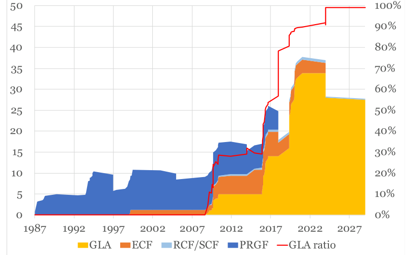
Note: Sources are IMF (2022) and Risk Control. Monetary amounts are in SDRs billions.
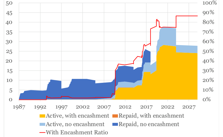
Note: Sources are IMF (2022a) and Risk Control.
7. Conclusion
In choosing whether to use their SDRs to generate MDB hybrid capital, holders are likely to be influenced:
1. By how effectively the reserve asset status of their holdings is maintained,
2. By the development leverage that different applications of lent SDRs can generate.
On the reserve asset status of SDRs employed as MDB hybrid capital, our calculations, based on a multiperiod Credit Portfolio Model (CPM) with parameters (PDs and LGDs) appropriate for lenders that enjoy strong Preferred Creditor Treatment (PCT), show that the probability of credit loss up to 20 years is negligible.
Pricing such hybrid capital, we find that a very low spread would be justified. Pricing matters because the importance that MDBs attribute to hybrid capital (it could completely transform the scale on which they are currently able to operate) means that they would likely be willing to exceed the fair spread by a significant margin. For central banks round the work managing their reserves, an investment in the form of MDB hybrid capital that yielded a spread exceeding the fair market spread, while still preserving Reserve Asset Status, would constitute an investment opportunity well worth exploring.
On liquidity, the PRGT liquidity arrangements provide a template for successfully maintaining this aspect of RAS when SDRs are lent for development finance purposes. These arrangements require participation by multiple donors and, if more than one MDB decides to issue hybrid capital, collaboration by the development banks themselves would appear advisable. Such coordination is likely to require significant engagement by G20 member governments both as MDB shareholders and potential SDR lenders. The transformational impact that hybrid capital could have on the scale at which MDBs operate would justify such engagement,
In the development leverage it generates, the MDB hybrid capital usage of SDRs performs well. If, as one might expect, MDBs manage their balance sheets conservatively following the issuance of hybrid capital, a single SDR of such capital will permit development lending at a rate equal to the current DRA to equity ratio under which the MDBs operate, namely around 3 to 1. In contrast, a single SDR lent to the PRGT or RST translates into just one SDR of final lending and, other things being equal, requires donations to create additional resources for the Reserve Account.
References
African Development Bank (2022) “MDBs as the Conduit of Choice for the IMF’s extraordinary SDR issuance,” mimeo.
African Development Bank and Interamerican Development Bank (2023) “Supporting sustainable development through SDR channeling to MDBs,” January.
Basel Committee on Banking Supervision (1998) “Enhancing Bank Transparency, Public disclosure and supervisory information that promote safety and soundness in banking systems,” September, available at https://www.bis.org/publ/bcbs41.htm
Basel Committee on Banking Supervision (2001) “Pillar 3 (Market Discipline), Consultative Document,” January, available at https://www.bis.org/publ/bcbsca10.pdf
Biglaiser, Glen, and Ronald J. McGauvran (2022) "The effects of IMF loan conditions on poverty in the developing world," Journal of International Relations and Development, 1-28, available at: https://doi.org/10.1057/s41268-022-00263-1.
Buiter, Willem H., and Steven M. Fries (2002) “What Should the Multilateral Development Banks Do?” EBRD Working Paper 74.
Cordella, Tito and Andrew Powell (2021) “Preferred and non-preferred creditors,” Journal of International Economics, 132.
Cox, John C. and Stephen A. Ross (1976) “The valuation of options for alternative stochastic processes,” Journal of Financial Economics, 3(1–2), January–March, 145-166.
Financial Stability Board (2013) “Principles for an Effective Risk Appetite Framework,” November, available at: https://www.fsb.org/2013/11/r_131118/.
Georgieva, Kristalina (2022) “Statement by Ms. Kristalina Georgieva, Managing Director of the IMF, 13th April, available at: https://www.imf.org/en/News/Articles/2022/04/13/pr22115-imf-md-welcomes-the-creation-ofthe-rst-to-help-vulnerable-countries.
G20 Capital Adequacy Framework Review (2022) “Boosting MDBs’ investing capacity - An Independent Review of Multilateral Development Banks’ Capital Adequacy Frameworks,” July, available at: https://g20.org/wpcontent/uploads/2022/07/CAF-Review-Report.pdf.
Harrison, Michael J. and David M. Kreps (1979) “Martingales and Arbitrage in Multiperiod Securities Markets,” Journal of Economic Theory, 20, 381-408.
Humphrey, Chris (2015) “Are Credit Rating Agencies Limiting the Operational Capacity of Multilateral Development Banks?” Inter-Governmental Group of 24, G24, October.
Jarrow, Robert A., David Lando and Stuart M. Turnbull (1997) “A Markov Model for the Term Structure of Credit Risk Spreads,” Review of Financial Studies, 10(2), 481–523.
International Monetary Fund (2009) “Balance of Payments and International Investment Position Manual, Sixth Edition,” available at: https://www.imf.org/external/pubs/ft/bop/2007/pdf/bpm6.pdf
International Monetary Fund (2013) “International Reserves and Foreign Currency Liquidity, Guidelines for a data template,” available at: https://www.imf.org/external/np/sta/ir/IRProcessWeb/pdf/guide2013.pdf
International Monetary Fund (2018) “IMF Financial Operations,” April, available at: https://www.elibrary.imf.org/view/book/9781484330876/9781484330876.xml?result=1&rskey=2XSyRr.
International Monetary Fund (2021) “IMF Conditionality, IMF Fact Sheet,” February, available at: https://www.imf.org/en/About/Factsheets/Sheets/2016/08/02/21/28/IMF-Conditionality.
International Monetary Fund (2022a) “2022 Review of Adequacy of Poverty Reduction and Growth Trust Finances,” April, available at: https://www.imf.org/en/Publications/Policy-Papers/Issues/2022/04/21/2022- Review-of-Adequacy-of-Poverty-Reduction-and-Growth-Trust-Finances-517091.
International Monetary Fund (2022b) “Proposal to establish a Resilience and Sustainability Trust,” IMF Policy Paper, April, available at: https://www.imf.org/en/Publications/Policy-Papers/Issues/2022/04/15/Proposal- To-Establish-A-Resilience-and-Sustainability-Trust-516692.
Khan, Mohsin S. and Sunil Sharma (2001) “IMF Conditionality and Country Ownership of Programs,” IMF Working Paper, WP 01/142, September, available at: https://www.imf.org/external/pubs/ft/wp/2001/wp01142.pdf.
Kolaric, Sascha, Florian Kiesel and Steven Ongena (2021) “Market Discipline through Credit Ratings and Too- Big-to-Fail in Banking”, Journal of Money, Credit and Banking, Vol. 53, Nos. 2-3 (March-April 2021), available at: https://onlinelibrary.wiley.com/doi/pdf/10.1111/jmcb.12789
Levy Yeyati, Eduardo (2009) “Optimal Debt? On the Insurance Value of International Debt Flows to Developing Countries,” Open Economies Review 20: 489-507.
Moody’s (2020) “Multilateral Development Banks and Other Supranational Entities, Rating Methodology,” October, available at: https://ratings.moodys.com/api/rmc-documents/69182.
Moody’s (2021) “African Development Bank – Aaa stable, Annual credit analysis,” October, available at: https://www.afdb.org/en/documents/moodys-rating-2021.
Perraudin, William, Andrew Powell and Peng Yang (2016) “Multilateral Development Bank Ratings and Preferred Creditor Status,” IDB Working Paper Series, No. IDBWP-697, Inter-American Development Bank (IDB), Washington, DC, available at: https://www.econstor.eu/bitstream/10419/146479/1/IDB-WP-697.pdf.
Perraudin, William and Peng Yang (2017) “Preferred Creditor Treatment and Risk Transfer,” Research Report N. 17/133a
Risk Control (2022) “MDB Sovereign Loan Credit Performance and PCT,” report prepared for the G20 CAF Review, May, available at: https://www.riskcontrollimited.com/insights/mdb-sovereign-loan-creditperformance-and-pct/
Risk Control (2023a) “Credit Term Structure Fits with Time Homogeneous Markov Chain Transition Matrices,” August.
Risk Control (2023b) “Pricing MDB Risk Transfers with Preferred Creditor Treatment,” (in preparation).
Schadler, Susan (2014) “The IMF’s Preferred Creditor Status: Does It Still Make Sense after the Euro Crisis?”, Center for International Governance Innovation, Policy Brief, No. 37, available at: https://www.cigionline.org/publications/imfs-preferred-creditor-status-does-it-still-make-sense-after-eurocrisis/
Schlegl, Matthias, Christoph Trebesch and Mark LJ Wright (2019) “The seniority structure of sovereign debt,” No. w25793, National Bureau of Economic Research, available at: https://www.nber.org/system/files/working_papers/w25793/w25793.pdf.
Standard & Poor’s (2021) Supranationals, Special Edition, October, available at: https://www.spglobal.com/ratings/en/research/pdf-articles/211027-supranationals-special-edition-2021- 100658635.
Standard & Poor’s (2023a) “Default, Transition, and Recovery: 2022 Annual Global Corporate Default And Rating Transition Study,” April, available at: https://www.spglobal.com/ratings/en/research/articles/230425default-transition-and-recovery-2022-annual-global-corporate-default-and-rating-transition-study-12702145.
Standard & Poor’s (2023b) “Default, Transition, and Recovery: 2022 Annual Global Sovereign Default And Rating Transition Study,” April, available at: https://www.spglobal.com/ratings/en/research/articles/230428default-transition-and-recovery-2022-annual-global-sovereign-default-and-rating-transition-study-12695994.
Stubbs, Thomas, Bernhard Reinsberg, Alexander Kentikelenis, and Lawrence King (2020) “How to evaluate the effects of IMF conditionality,” The Review of International Organizations, 15, 29–73, available at: https://doi.org/10.1007/s11558-018-9332-5.
Appendix: MDB Balance Sheet Data
Table A1: MDB Bank Balance Sheet and Financial Ratios AfDB IDB
Development Assets EAD 26,363 121,468
Non-development Assets EAD 14,768 29,228
Total Assets EAD 41,131 150,697
Equity 9,883 37,873
Development Assets to Total Assets 64.1% 80.6%
Development Assets to Equity 2.67x 3.21x
Total Assets to Equity 4.16x 3.98x
Non-development Assets to Development Assets 56.0% 24.1% Note: For AfDB, the values are in millions UA. For IDB, the values are in millions USD.
Risk Control 13-14 Dean Street London W1D 3RS +44(0)2033070730 www.riskcontrollimited.com
Notes
[1] The 20 prescribed holders of SDRs are 4 central banks (European Central Bank, Bank of Central African States, Central Bank of West African States, and Eastern Caribbean Central Bank); 3 intergovernmental monetary institutions (Bank for International Settlements, Latin American Reserve Fund, and Arab Monetary Fund); and 13 development institutions (African Development Bank, African Development Fund, Asian Development Bank, Caribbean Development Bank, the Development Bank of Latin America (known as Corporación Andina de Fomento), the European Bank for Reconstruction and Development, the European Investment Bank, Inter-American Development Bank, International Bank for Reconstruction and Development and the International Development Association, Islamic Development Bank, Nordic Investment Bank, and International Fund for Agricultural Development).
[2] See https://www.imf.org/en/About/FAQ/Resilience-and-Sustainability-Trust#Q2
[3] Risk Control is a specialised, quantitative, advisory firm that works with multilaterals on a range of technical, financial, and modelling issues.
[4] For each bank, the simulation is performed using the initial portfolio composition (in the exercise presented this corresponds to the end 2022 portfolios). In this, it assumes that exposures to different names are replaced with similar exposures in future. When an exposure defaults, we suppose that a provision is recorded. Additionally, we assume that there is a 20bps income each period to cover some provisions. We cumulate the provisions minus the spread income over time and compare their sum to the par value of the original portfolio. Our approach may be viewed as appropriate for lenders such as MDBs which lend at highly favourable spreads. The assumption of a 20 bps spread represents a ‘conservative’ estimate of the Expected Loss (EL) on the credit risky loans and is net of administrative or overhead costs of investing in the loans. By ‘conservative’, we here mean low since a higher spread would create additional resources to offset against the loan provisions, making it less likely that the hybrid capital would become loss absorbing.
[5] MDBs are at the forefront of the implementation of the UN SDGs. It should be verified that that the new SNA is consistent with the hybrid capital instrument described in the MDB Proposal.
[6] BMP6, 6.69 adds “This concept refers to both non-marketable assets, such as demand deposits, and marketable assets, such as securities for which there are ready and willing seller and buyers. The ability to raise funds by using the asset as collateral is not sufficient to make an asset a reserve asset. Some deposits and loans can be liquid and included in reserve assets, although they are not necessarily marketable.”
[7] On Deposit Account claims on the RST, it is stated that: “DA claims. […] Liquidity of contributors’ claims on the DA would be ensured by investing DA deposit resources in high quality instruments, with sufficient liquidity of the asset pool to allow for encashment of individual contributors’ claims when they experience a BoP/reserve need. A contributor encashing their claim on the DA would commit to reconstituting its deposit once it no longer has a BoP need.” Source: IMF (2022b).
[8] As stated in the latest G20 CAF Review (2022), capital adequacy measures a financial institution’s ability to honor its financial obligations if its debtors are unable to pay back what they borrowed. Measures can be risk-based (e.g., using risk- weights) or focus on financial leverage, which considers an MDB’s capital and non-risk-adjusted assets.
[99] Among the more prominent investors in MDB bonds are leading central banks. Some countries have argued that for their central banks to invest in MDB hybrid capital would be counter to the intended purpose of SDRs, while their central banks are simultaneously investing in MDB bonds.
[10] The inverse of this ratio is known as the Capital Adequacy Ratio (CAR) or Capital Coverage Ratio (CCR).
[11] The latest thinking of the MDBs considering SDR-based hybrid capital is that they may use the Total Assets ratio alone.
[12] To be more precise, historical data, in our experience MDB LGDs are generally lower on average than 10%. The LGD experienced reflects the level of interest rates that pertains when the sovereign is in default. Since almost all sovereigns repay MDBs the principal and interest arrears when they remerge from default, the primary source of loss, in most cases, is the forgone ‘interest on the interest’. Calculations and a discussion of sovereign LGDs experienced by MDBs may be found in Risk Control (2022).
[13] The fiscal year 2020 data cited here have not been updated in subsequent Moody’s publications and, hence, are not readily obtainable for later years.
[14] It is equal to the sum of square of the exposure weights.
[15] So, a granularity of 20 means that the portfolio has the concentration pattern of a portfolio made up of 20 equal-sized exposures.
[16] The AfDB has, in fact, the same granularity as the IBRD, which covers many more regions.
[17] If a private sector lender were to provide financing to emerging market borrowers, they would require extremely large spreads as remuneration. These could be large enough for such lending to be economically viable so the very large PLs in the upper part of the table do not mean that no private sector financing solutions are viable. Nevertheless, they do serve to underline the extreme importance of PCT in evaluating lending by institutions like MDBs.
[18] The Treasury Assets/DRA for IDB and AfDB are 24.06% and 56.02%. The percentage losses that we associate with the total asset trigger events are then 18.10% and 11.24%, respectively.
[19] By ‘fairly priced’, we mean that it inclusive of appropriate allowance for expected losses and a premium for risk.
[20] This approach is consistent with common practice in debt valuation since few market participants attempt direct modelling of work-out or liquidation processes but instead employ a summary loss given default.
[21] In constructing the graph, we have assumed that all borrowing contracts are bullets.
[22] The arrangements proposed by AfDB and IDB may possibly differ from this in that countries may have an obligation rather than an option to respond to a request for support.