

1. Introduction
This note presents bank default probabilities in the Covid-19 crisis in the form of regional indices for North America, Europe, Africa, Asia & Oceania, Latin America & Caribbean and Middle East.
The indices are based on individual bank default probabilities for a large number of banks worldwide. These are estimated using an equity-based model in which the bank’s equity market capitalisation divided by total debt resembles a perpetual American call option. Using this approach, we estimate the probability of default for a given horizon (say five years) as the probability that the bank’s asset to debt ration crosses a threshold before the horizon in question.
The statistical implementation is performed rigorously using Maximum Likelihood techniques. (Equity divided by debt is modelled as a function of the asset to debt ratio. The likelihood is related to that of a bivariate geometric Brownian motion in which the first element is absorbed as a barrier.)
We focus on how the credit quality of banks for particular regions has changed since the onset of the crisis. From the indices, one may examine how much the major deterioration in bank credit quality that occurred in Q2 2020 has persisted in different regions in Q2 and early Q3 2020.
The note is organised as follows. Section 2 discusses the methodology (in non-technical terms) and data. Section 3 describes the PD calculation results. An appendix provides technical information about the methodology employed.
2. Methodology and Data
2.1 Methodology for Estimating Default Probabilities
This section describes the methodology employed in non-technical terms. Mathematical details of the modelling approach are set out in an appendix.
It is common to think of bank credit quality as based on ratios of capital to risk weighted assets. The notion of capital employed in such calculations is based on accounting measures of book equity adjusted for retained earnings, provisions and write-offs. It is possible using market data to estimate a more forward-looking notion of equity equal to the difference between the market value of assets minus that of liabilities.
If one (i) assumes that a firm will default when its assets (expressed in market value terms) fall below a given fraction of its liabilities, and (ii) estimates the likelihood that the asset to liability ratio declines below a proportional constant, then one can estimate statistically the probability of default.[1]
In broad terms this is the approach taken in this note. We construct a dataset comprising time series information on the equity market capitalisation and total debt for a large number of banks worldwide. We formulate a continuous time model of the evolution of equity market to debt values using Merton’s insight that a firm’s equity is a call option on its underlying assets (expressed in market value terms). Our model is an ‘American option’ model in which defaults may occur at any time, not just at a given fixed future date. (If one is prepared to make the latter unrealistic assumption, a simpler ‘European option model’ may be used.)
We implement the above described model statistically using a rigorous Maximum Likelihood approach. We believe this is superior to the approximations commonly used in the literature in which equity volatilities are assumed to be constant. Our methods also directly estimate risk premia based on correlations between log returns on underlying asset values and the log return on an equity index.
Having obtained time series of default probabilities for large numbers of individual banks, we construct country-level indices by weighting individual bank default probabilities by liability levels. We aggregate the country-level indices for a set of regions, namely North America, Europe, Africa, Asia & Oceania, Latin America & Caribbean and Middle East, weighting the country-level indices by real GDP. (This GDP-based weighting is preferable to weighting by total country-level liabilities because the currencies of countries in crisis typically drop substantially so their banks contribute little to liability-weighted results.[2]
2.2 Data Employed
The equity model described above is estimated using a dataset of information about global banks obtained from Refinitiv Eikon. All banks selected are currently listed on the stock market. The number of countries and banks included in each region is summarized in Table 1.
Four time series in the dataset are employed in our estimation.
| Number | Number | |
|---|---|---|
| Region | banks | countries |
| Africa | 55 | 13 |
| Asia & Oceania | 299 | 18 |
| Europe | 178 | 30 |
| Latin America & Caribbean | 57 | 10 |
| Middle East | 104 | 9 |
| North America | 402 | 2 |
| Total | 1,095 | 82 |
Note: There are 82 countries and 1,095 banks in total used in the final dataset for the estimation.
1. Market capitalization
Market capitalization represents the sum of market value for all relevant issue-level share types of the bank. The issue-level market value is calculated by multiplying the requested share type by the latest close price. Market capitalization data is in daily frequency.
2. Total liabilities
Total liabilities include total current liabilities, total long-term debt, deferred income tax, minority interest and other liabilities. Total liabilities data is in annual frequency. Weekly time series on liabilities are generated via linear interpolation.
3. Market portfolio
We use the MSCI All Country World Index (ACWI) as market portfolio. “The MSCI ACWI captures large and mid-cap representation across 23 Developed Markets (DM) and 26 Emerging Markets (EM) countries. With 2,988 constituents, the index covers approximately 85% of the global investable equity opportunity set”.[3] The index is denominated in USD and available in daily frequency.
4. Dividend payment dates
Dividend payment dates are the dates in history when the dividend is payable to the shareholders.
The sample period employed in our estimations runs from 01/01/2017 to 31/12/2019 and consists of 3-years of weekly observations. Observations on the dividend payment dates and with weekly market capital change greater than 5% are dropped from the estimation.
3. Estimation Results
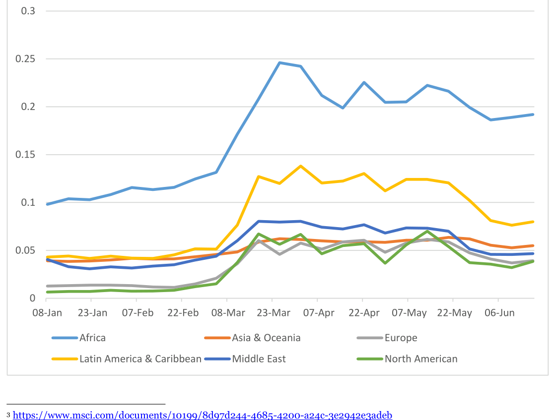
This section presents regional indices of 5-year bank default probabilities in the Covid-19 crisis. Figure 1 shows the time series of estimated PDs from the beginning of 2020 till June 2020. The data shows a wide variation in default probabilities by region in January and February 2020. Bank default probabilities in North America are low at around 1%. The level of PDs for Middle East, Asia & Oceania and Latina America & Caribbean (LAC) are at medium levels of between 2.5 and 5%. Default probabilities for African banks are high at around 8% at the start of the year.
The first three weeks of March see sharp increases in bank default probabilities in all regions. In riskier regions such as Africa and LAC, default probabilities more or less double the early March levels whereas for low risk regions the proportional increases are greater. The Asia & Oceania region exhibits a relatively small proportional increase.
Since late May, default probabilities in LAC have declined noticeably. Bank default probabilities in Africa have decreased slightly but remain high. PDs for North American banks have exhibited some monthly volatility but have recovered somewhat since their peak in mid-May.
Table 2 presents weighted averages of key bank level quantities that are intermediate outputs from the calculation of default probabilities. These are (i) the level of asset value to total liabilities at the end of the sample period, k[0], and (ii) the (annualized) volatility or standard deviation of log changes in the asset to liability ratio. The former quantity represents the net worth of the bank proportional to total liabilities while the latter reflects the riskiness of the underlying assets.
As one may observe, some regions like LAC and the Middle East have high net worth Asia & Oceania and relatively high risk. Risk is particularly high in LAC. European banks exhibit the lowest proportional net worth but also very low underlying asset risk. African banks have relatively high risk but proportional net worth lower than, for example, the Middle East banks. North American banks have higher asset risk than European and Asia & Oceania banks but higher proportional net worth.
| Latin | |||||
|---|---|---|---|---|---|
| Asia & | America & | Middle | North | ||
| Africa | Oceania | Europe | Caribbean | East | America |
| 1.088 | 1.062 | 1.032 | 1.162 | 1.146 | 1.084 |
| 0.033 | 0.018 | 0.013 | 0.045 | 0.032 | 0.028 |
Note: The weighted average is calculated in the same way as averaged PDs as described in equation (22) and (23).
References
Cox, D., and Miller (1973) The Theory of Stochastic Processes.
Ronn, Ehud I., and Avinash K. Verma (1986) “Pricing Risk-Adjusted Deposit Insurance: An Option-Based Model,” Journal of Finance, 41(1) September 871-895.
Appendix: Methodology
Equity-based model This section sets out the modelling framework employed. The approach is technical and some readers may wish to proceed to the next section which describes the data and results.
Assume a firm has the earnings flow: δ (Vt −Dt) (1)
Here, Vt is the value of the firm’s underlying assets, Dt is the firm’s total liabilities, and δ is a constant dividend pay-out rate.
We assume Vt, Dt and the market portfolio, Mt are described by the following set of geometric Brownian motions. dVt = μvVtdt+ σvVtdW1t (2) dDt = μDDtdt (3) dMt = μmMtdt+ σmMtdW2t (4)
Here, dW1tdW2t = ρdt, ρ is the correlation between the market and the firm’s asset value. We also assume the ∗ = r−δ, short-interest rate is constant and equal to r. The risk-adjusted drift terms for Vt, Dt and Mt are: μv ∗ = r, respectively. We suppose that a representative agent has log utility and obtain the μD∗ = r−δ and μm 2 .[4] actual equilibrium drift terms for our processes as: μv = r−δ+ σvσmρ, μD = r−δ and μm = r+ σm
By standard stochastic calculus arguments, we can derive the process followed by the firm’s total value equity, Xt = X(Vt, Dt), which by risk-neutral argument must satisfy:
∂X ∂X σv2 ∗V rX= δ(V−D) + μv ∂V + μDD ∂D +[2] V[2] ∂V∂[2]X[2] (5)
Suppose that insolvency occurs when the ratio of assets to liabilities kt ≡Vt/Dt falls below an exogenous trigger level, k, and that equity-holders receive nothing in the insolvency settlement.
In the estimation and calculation of default probabilities reported in this note, we set k equal to 0.97. This choice is consistent with the approach taken by Ronn and Verma (1986) in their classic study of deposit insurance valuation.
Using the homogeneity of equation (5) and dividing quantities by liabilities D, we can obtain a simple solution to Y(k) = X(k, 1) rather than to X= X(V−D), where Y(k) is the equity to liability ratio. Changing variables and by using appropriate boundary conditions: (i) lim k→k Y(k) = 0, when insolvency occurs and (ii) k→∞lim Y(k) = k−1 when deposits become risk free, one obtains the simple solution:
λ k Y(k) = k−1 −(k−1) ( (6) k)
1 σv2 λ= 2 −√σ[4]v4 + 2σv2δ) (7) σv2 (
One should note that under our assumptions, only the ratio of assets to liabilities matters for such quantities as the probability of default. If deposits or assets followed more general processes than geometric Brownian motions, these variables would in general remain as separate state variables, affecting default probabilities separately.
The value of the equity-holders’ limited liability option per dollar of deposits, denoted G(kt), is the non-linear term in (6), i.e., λ k (8) G(kt) = (k−1) (k)
Suppose that the firm is charged a deposit insurance premium γ per dollar of deposits and per time period. To ascertain the actuarially fair level of γ under the simplifying assumption that all the deposits are fully guaranteed, one may set the unlimited liability value of the firm equity k−1 equal to the firm equity level when insolvency is possible and when a premium is paid: k−1 −γ/δ−(k−1 −γ/δ)(k/k)λ . Rearranging, one obtains:
δ(1−k)(k0/k)λ γ= 1−(k[0]/k)λ (9)
Here, the actuarially-fair γ depends upon an initial level of the asset-to-liabilities ratio, here denoted k[0].
The Likelihood estimation with absorbing barrier To estimate the parameters of the processes followed by each firm’s asset-liability ratio, kt, Maximum Likelihood (ML) methods are employed.
Recall that the logs of assets to liabilities ratio and the market portfolio comprise a bivariate arithmetic Brownian motion:
dlog(kt) = (r−δ−μD + σvσmρ−σv[2]/2)dt+ σvdW1t (10) dlog(Mt) = (r+ σm[2] /2)dt+ σmdW2t (11) Here, dW1tdW2t = ρdt.
Let the vector process be denoted xt ≡(x1t, x2t, … , xnt)′ and suppose that:
′ , i= 1,2, … , n (12) dxit = μidt+ σidBit
Bit′ , i= 1,2, … , n are standard Brownian motions and dBit′ dBjt′ = ρijdt. Also suppose that x1t is absorbed at a. Let ψ(xt, t|xt0) be the conditional density of xt given xt0. ψ satisfies the following Kolmogorov forward equation:
∂ψ n ∂ψ n n σiσjρij ∂2ψ ∑ μi i=1 i=1 j=1 ∂t = −∑ ∂xit + ∑[2] ∂xit∂xjt (13)
Subject to the two boundary conditions are (i) ψ(a, x2t, … , xnt, t|xt0) = 0 for all (x2t, … , xnt) and t, and (ii) ψ(xt0, t[0]|xt0) = δ(xt0), where δ is a Dirac delta function (for discussions of such forward equations, see Cox and Miller (1973)). Henceforth, for simplicity of exposition, we normalise so that xit0 = 0 for all i.
The solution for the bivariate case is ψ(xt, t|0n) = |det (Σ)|−1/2(exp{−1/2(xt −μt)′(1/t)Σ −1(xt −μt)} − exp(ζ) exp{−1/2(xt −φ−μt)′(1/t)Σ −1(xt −φ−μt)}) (14)
where 0n is an n-vector of zeros, φ[1] = 2a, and φ[2] = 2aσ[2]ρ1,2/σ[1] a= log(k) −log (k[0]), and ζ= φ′Σ −1μ, μ= (μ[1], μ[2])′ and
σ1 σ1σ2ρ1,2 Σ ≡[[2] ] (15) σ1σ2ρ1,2 σ2
The likelihood function is constructed as follow. T L= ∑t=1 ψ(xt, t|0n) (16)
T −log(L) = −∏t=1 ψ(xt, t|0n) (17)
Here, T is the number of weekly observations. The parameters σ[1], σ[2] and ρ1,2 are estimated by minimizing equation (17).
Analytical calculation of PDs Having estimated the parameters involved in the processes, one can calculate firms’ PDs using an analytical formula derived from equation (14).
To simplify the calculation, rewrite (14) into the density function of one variable (asset to liability ratio) case:
2 2 1 1 x−μkt 2aμk 1 x−2a−μkt p(x, t) = } −exp( ) }] σk√t√2π [exp{−[2] ( σk√t ) σk[2] ) exp{−[2] ( σk√t (18) 2 2 1 1 x−μkt 2aμk 1 1 x−2a−μkt = } −exp( ) } 2 ( 2 ( σk√t√2π exp{− σk√t ) σk2 ) σk√t√2π exp{− σk√t
2/2. Here, a= log(k) −log (k[0]), k is the trigger level, k[0] is the initial asset to liability ratio, μk = 4σkσmρk,m −σk σk and σm are annualized.
The probability of survival can be expressed as:
∞ P(survival, t) = ∫a p(x, t)dx 2 2 ∞ 1 1 x−μkt 2aμk ∞ 1 1 x−2a−μkt = ∫a σk√t√2π exp{−[2] ( σk√t ) } dx −exp( σk[2] ) ∫a σk√t√2π exp{−[2] ( σk√t ) } dx (19) a−μkt 2aμk −a−μkt = 1 −Φ ( σk√t ) −exp( σk[2] ) [1 −Φ ( σk√t )]
Here, Φ(. ) is the cumulative distribution function of a standard normal distribution.
The probability of default in t-year is:
a−μkt 2aμk −a−μkt PD(t) = 1 − P(survival, t) = Φ ( σk√t ) + exp( σk[2] ) [1 −Φ ( σk√t )] (20)
The one-year probability of default is simplified as:
a−μk 2aμk −a−μk PD= Φ ( σk ) + exp( σk[2] ) [1 −Φ ( σk )] (21)
Weighted Average PDs The region PDs are estimated in two steps:
1. Estimate the PDs for individual countries in each region. The PDs for a particular country c are estimated by the weighted average PDs of banks in country c.
N (22) PDc = ∑i=1 wiPDi
Li Here, N is the number of banks in country c, wi = ∑Nj=1Lj, Li is the liability amount of bank i in country c, PDi is the PD for bank i estimated using equation (20).
2. Estimate the weighted average PDs for each region.
M (23) PDr = ∑c=1 wcPDc
GDPc M where M is the number of countries in region r, wc = ∑k=1GDPk, GDPc is the latest available GDP for country c obtained from The World Bank website.
The annual liabilities observations are up to 2019. To calculate PDs in 2020, we assume firms’ liabilities are unchanged since the end of 2019.
Risk Control Limited 13-14 Dean Street London W1D 3RS +44 (0)203 307 0730 www.riskcontrollimited.com
Notes
[1] The classic study of deposit insurance valuation, Ronn and Verma (1986) sets this constant to 0.97. We follow their approach here.
[2] For example, if one used liability weighted default probabilities in Latin America currently, Argentine banks would receive a very low weight because of the weakness of the Argentine peso.
[4] We assume δ= 0.03 and r= 0.05 in our calculation.