

This paper generalizes a class of ratings-based credit derivative models proposed by Jarrow, Lando, and Turnbull (1997) and Kijima and Komoribayashi (1998) to allow for stochastic spreads and then applies this model to analyze empirically the pricing of large cross sections of corporate bonds and Asset Backed Securities. We show that measuring risk in credit portfolios is highly sensitive to the inclusion of randomness in spreads.
Research Paper
Ratings-Based Pricing and Stochastic Spreads
Date:2008 Reference Number:8/2
Ratings-Based Pricing and Stochastic Spreads
Mariam Harfush-Pardo Robert Lamb Risk Control Limited Imperial College
William Perraudin Imperial College
September, 2007∗
1 Introduction
The nature and determinants of credit spreads are the subject of a substantial and growing empirical literature. Researchers have investigated spreads using equity-based models (Delianedis and Geske (2002), Huang and Huang (2002) and Eom, Helwege, and Huang (2004)), hazard models (Duffie and Singleton (1997), Duffie and Singleton (1999) and Driessen (2005)) and CAPM/APT asset pricing models (Elton, Gruber, Agrawal, and Mann (2001)). Recently, several authors have looked at liquidity effects in corporate credit markets (Ericsson and Renault (2006), Longstaff, Mithal, and Neis (2005), de Jong and Driessen (2006) and Perraudin and Taylor (2007)).
This paper is the first, to our knowledge, to investigate spreads empirically using a ratings-based credit risk pricing model. Ratings based models were introduced by Jarrow, Lando, and Turnbull (1997) and Lando (1998) and extended by Kijima and Komoribayashi (1998). Related to hazard-based reduced form models like those of Duffie and Singleton (1997), Duffie and Singleton (1999), ratings-based models suppose that credit quality is described by an exposure’s rating and that, on a risk-adjusted basis, ratings follow a Markov chain. If the Markov chain is formulated in continuous time, the key focus is on the ratings’ risk adjusted transition matrix. If a continuous time approach is employed, the key concept is the set of hazard rates that describe the likelihood of transitions between ratings.
Both the Jarrow, Lando, and Turnbull (1997) and Kijima and Komoribayashi
(1998) models formulate risk-adjusted transition matrices by perturbing a historical transition matrix in ways that depend on vector of rating-specific prices of risk for each maturity. The historical matrix is then estimated from data on actual ratings transitions while the prices of risk as chosen so as to fit the current credit term structures for differently rated bonds.
The basic Jarrow-Lando-Turnbull model and the Kijima and Komoribayashi model do not allow for stochastically evolving spreads for given rating categories. Jarrow, Lando and Turnbull show how their model may be generalized to a continuous-time diffusion framework in which rating-specific hazards of changes in ratings evolve over time. Lando (1998) provides a systematic exploration of this model. These diffusion-based models do imply stochastic spreads but it is not straightforward to solve for hazard rates from observed spreads and vice versa.
In this paper, we show how one may straightforwardly generalize discrete time ratings based models to allow for stochastic credit spreads. For each future date, “forward default probabilities” are chosen to match the current term structure of credit spreads. As conditional probabilities, these evolve as martingale processes under the risk neutral measure and their evolution then induces stochastic time-variation in spreads. The model provides an analytically tractable way of valuing securities and performing risk simulations in a ratings-based discrete time framework with stochastic spreads.
We implement our model using spread data by rating and maturity extracted from large cross sections of corporate bond and Asset Backed Security (ABS) prices. The spreads are extracted using techniques developed by Harfush-Pardo, Perraudin, and Taylor (2007).
We find, first, that the spreads exhibit interesting patterns of segmentation in that different sections of the market distinguished either by ratings or maturity ranges are more or less correlated with other parts of the market. Second, it is noticeable that the risk adjusted forward default probabilities associated with particular future years decline over time. We interpret this as reflecting a risk premium associated with shocks to spreads.
Ratings-based models supplemented with assumptions about the correlation of ratings transitions are widely used as a framework for measuring solvency risks in financial institutions. It is interesting to quantify how much the introduction of spread risk affects risk calculations on portfolios of credit exposures. In the last section of the paper, we simulate loss distributions for realistic bond portfolios and study how risk statistics are affected by the inclusion of stochastic spreads.
2 Model Description
2.1 Notation
To be precise, Jarrow, Lando, and Turnbull (1997) suppose that the risk-adjusted matrix for each future period is the historical matrix with probability shifted off the diagonal to other elements in a way that is proportional to a price of risk.
Suppose at date t we observe a set of spreads St,j(k) for different rating categories k = 1, 2, ..., N and maturities j = 1, 2, .... Let γ be the expected recovery rate and assume that shocks to the interest rates and those to credit risk are independent. Under these assumptions, it follows that: h i ¡ ¢ £ ¡ ¢¤ exp St,j(k)j = Prob∗t τd > t + j|k + γ 1 − Prob∗t τd > t + j|k (1)
Here, Prob∗t(.) denotes the risk-adjusted probability conditional on information at date t. Also, τd is the random time at which default occurs. Let Q(t,jk) denote the probability of default between t and t + j conditional on information at t. Then: t,j j] Q(t,jk) ≡ Prob (τ ∗ ∈{t, t + 1, ..., t + j}) = 1 − exp[−S(k) (2) 1 − γ Let q(k)t,j be the probability that default occur between t+j-1 and t+j conditional on information at t and in particular conditional on the fact that the exposure has a rating k at t.
qt,j(k) = Probt(τ d = t + j|rating at t = k) = Q(k)t,j − Q(k)t,j−[1]. (3) h i The probabilities for different ratings are denoted qt,j(k) ≡ qt,j(1), qt,j(2), . . . , qt,j(N) .
2.2 Structure of the Transition Matrices
Now, we impose some structure on the risk-adjusted ratings transition matrix that will prove useful. Suppose that the risk-adjusted distribution of ratings changes conditional on information at t is described by a set of one-period transition matrices Mt,[1], Mt,[2], . . .. The (k, l)th element of Mt,j represents the probability that an obligor rated k at t + j − 1 will be rated l at t + j. Again without loss of generality, we can write Mt,j in partitioned form as:

Mt,j(−d) ... Mt,j(d) (4) . . . . . . . . . . . .

0 ... 1
Where Mt,j(−d) is N × N and Mt,j(d) is N × 1. For any M dimensional vector v, adopt the notation:

0 . . . 0 v[1] 0 v[2] . . . 0 I(v) = (5) ... ... ... ...
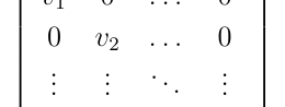
0 . . . 0 vM is an N × N diagonal matrix for any N−vector v = (v[1], v[2], ..., vN)′.
Assumption 1 Now, suppose Mt,j(−d) has the form:
Mt,j(−d) ≡ I(1N − Mt,j(d))M˜ (6)
where M˜ is invertible.
Here, note that M˜ is time homogenous and may be interpreted as the rating transition matrix for an exposure conditional on no default.
Proposition 1 Under Assumption 1, one may derive an explicit expression for the forward default probabilities conditional on information at t as a function of observed spreads:

1 − exp[−St,(1)[1] (j)]
![Equation: Mt,(d[1]) = ... (7)](/api/media/file/eq-223-300x16.png?prefix=media)
1 − γ 1 − exp[−St,(N[1] )(j)]

exp[−S(1) Yj−[1] ³ ´−[1] t,j−[1](j − 1)] − exp[−St,j(1)(j)]

1 − γ k=1 exp[−St,j(N−)[1](j − 1)] − exp[−St,j(N)(j)] for j = 2, 3, . . . ,
Conversely, the spreads St,j(n) are uniquely determined by the forward default probabilities Mt,j(d).
2.3 Fitting Observed Spreads
The above model provides a consistent set of risk-adjusted distributions for future ratings. If credit risk is entirely described by the evolution of ratings, one may employ this framework to price credit-sensitive exposures by calculating discounted, expected payoffs. Given a time homogeneous matrix, M˜ , one may also benchmark the distributions from a single cross section of spreads observed at date t (St,j(n) for j = 1, 2, . . . and n = 1, 2, . . . , N) by choosing the M (t,jd) appropriately. In practice, fitting to a set of spreads using equation (7) may yield Mt,j(d) that are not monotonically increasing in d. In other words, for some future date t + j the forward default probability for one rating k may be lower than that for a lower credit quality rating l > k. Hence, to benchmark offspread data requires that one perform a constrained minimization of the form: h ³n X o´i[2] min St,j(n) − h Mt,j(d) , j = 1, 2, . . . , J , n = 1, . . . , N Mt,j(d) j = 1, . . . , J j = 1, 2, . . . n = 1, . . . N n = 1, . . . , N subject to Mt,j,n(d) > M (t,j,nd) +1 for all j = 1, 2, . . . n = 1, . . . , N − 1 . (8)
Here, h(.) is the mapping from the Mt,j(d) to the St,j implied by the inverse of the function given in equation (7).
The risk adjusted distributions specified in Assumption 1 imply that, while spreads may change over time, they will do so in a non-stochastic way that is fully predictable at some initial date 0. To see how spreads will vary, note that the distribution of ratings at a future date j conditional on information at 0 is given by a set of transition matrices: " # " # " # " # Mt,(−1d) Mt,(d1) Mt,(−2d) Mt,(d2) Mt,j(−d)1 Mt,j(d)−1 Mt,j(−d) Mt,j(d) , , . . . , , 0′N 1 0′N 1 0′N 1 0′N 1 (9) To take an example, at date zero, the two year maturity spreads will be determined by the product of the left hand two matrices in this sequence. At date, j − 2, the two year spreads will be determined by the product of the last two matrices in the sequence. Hence the two years at date j − 2 will be known at 0 and will differ from those observed at that date.
One may deduce the following proposition:
Proposition 2 Under Assumption 1, spreads St,j(n) for ratings n = 1, 2, . . . , N, and maturities j = 1, 2, . . . are constant over time t = 1, 2, . . . if and only if the forward default probabilities are constant over time for any given j, i.e.,
Mt([1]d,j) = M (t[2]d,j) (10)
for all t[1] and t[2].
2.4 Stochastic Spreads
Our approach may be generalized straightforwardly to the case in which spreads evolve stochastically by allowing the Mt,j,d to be random. Stochastic evolution in Mt,j,d implies evolution in the risk adjusted transition matrices that market participants use to price credit-sensitive claims and hence stochastic variation over time in spreads. It is important that Mt,j,dk < M kt,j,d+1 for all k = 1, 2, ..., N, i.e. that default probabilities increase as the credit quality decreases. A simple way to ensure this is to suppose that Mt,j,dk are given from initial spreads and that

Mt1+1,j−1,d Mt,j,d1 Mt2+1,j−1,d Mt,j,d2 (11) = ηt+1,j−1 ... ...

MtN+1,j−1,d Mt,j,dN where ηt+1,j−[1] is a common shock affecting all rating categories for a particular future maturity and where
(12) Et(ηt+1,j−[1]) = 1 for all t, j.
forward default probabilities for different ratings but the same future date will be perfectly correlated using this approach. But the term structure of credit spreads may still be driven by a large number of factors as there may be up to as factors as maturities considered.
3 Empirical Implementation
3.1 Data
To implement this approach, we begin by estimating spreads for different ratings categories and maturities. The standard way to accomplish this is to fit the discount functions implicit in a data set of individual bond prices using nonlinear functions of maturity. Functions commonly used include cubic splines or weighted averages of exponentials such as those employed in the Nelson-Siegel approach. The obvious drawback of this approach when applied to credit spreads for specific ratings categories is that the term structures for adjacent ratings categories may cross.
Harfush-Pardo, Perraudin, and Taylor (2007) develop techniques for estimating credit term structures for multiple ratings categories and we apply their approach here. In brief, we estimate defaultable bond term structures on a given date for different ratings categories by performing a least squares fit of the crosssection of bond prices to the values implied by a risk-adjusted ratings transition matrix. We impose simple constraints on the risk-adjusted transition matrix to ensure that the implied credit term structures do not cross for different ratings categories. More details on the extraction of ratings-specific term structures are given in the Appendix.
The corporate bond data we employ consists of 50 monthly cross sections of the prices of US straight bonds denominated in US dollars. The data set contains approximately 9,500 bonds in total but available to estimate each cross section varies. The government bond yields are the US constant maturity yields published by the Federal Reserve Board. We interpolate these rates so that we can obtain the interest rates for all integer maturities: 1,2,,30 years.
We value ABS by treating them as balloon bonds with maturity equal to the weighted average life reported by Reuters. To estimate the spreads for ABS, we use the same procedure described above that we used for corporate bonds.
The ABS data we employ is based on monthly time series of cross sections of dollar denominated tranches listed in the Merrill Lynch ABS Index (fixed rate) from June 2002 to September 2006. The Merrill Lynch index is composed only of investment grade ABS. The total sample is composed of 92,708 observations of which 67% are AAA bonds, 12% AA, 12% A and 8% BBB. Monthly snap-shots have at least 700 observations.
The proportion of observations by maturity is shown in Table 1. As we can see in Table 1, 80% of the observations have a maturity less than 5 years. Table 2 shows the proportion of observations by ABS sector. For a given rating category, there is evidence that the market prices ABSs from different sectors differentially.
In future work, we intend to investigate this.
4 Empirical Results
4.1 Term Structures
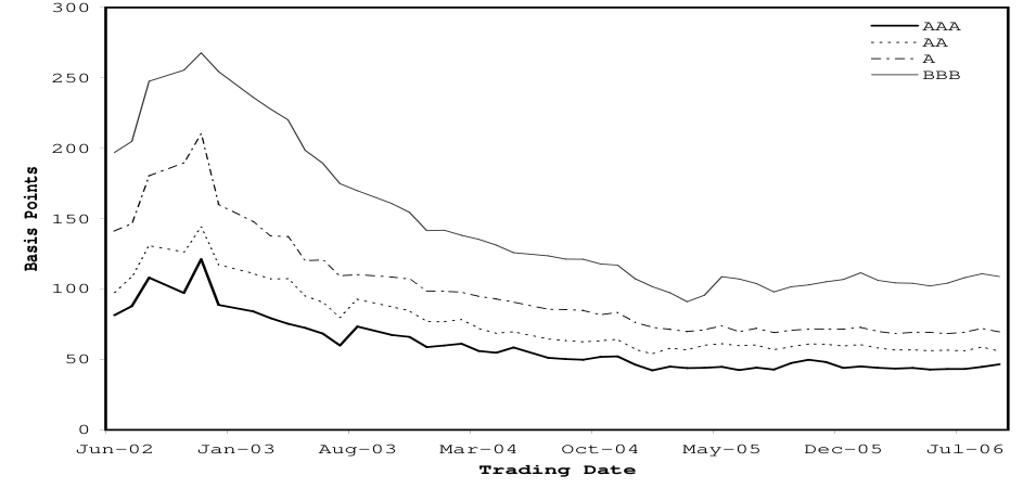
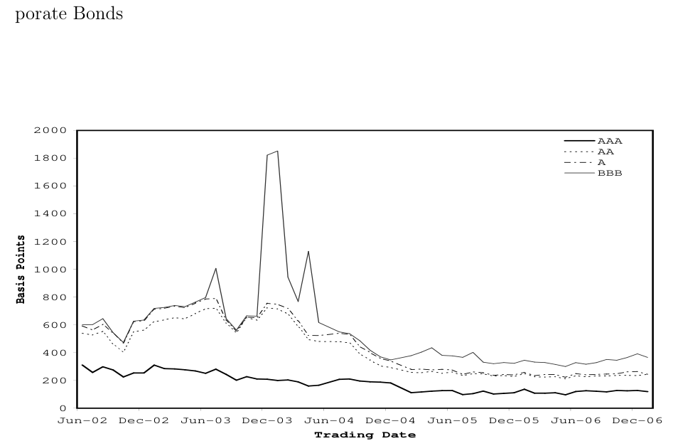
Figures 1 and 2 show representative sets of corporate bond spread term structures for 2-year and 5-year maturity investment-grade corporate bonds. While the term structures move broadly together, one should note the periods in which discrepancies are evident. For example in 2002, for over a period of about a quarter AAA and AA spreads were falling while those on A and BBB rose. The converse happened over a 2 month period in the summer of 2003. These divergent spread changes are apparent in both 2- and 5-year spreads.
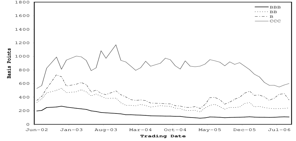
Figures 3 and 4 show term structures for sub-investment-grade corporate bonds. These behave very differently over time from the investment grade spreads. BB- and B- grade spreads rise significantly from mid 2005 at a time when investment grade spreads are flat. CCC spreads remain high in early 2003 when other spreads are falling and then fall sharply from late 2004 when low B-grade spreads are rising. Again, the movements in 2- and 5-year maturity sub-investment-grade spreads are quite similar.
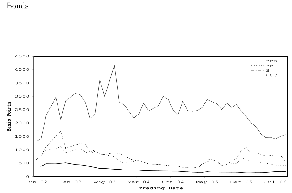
Figure 5 shows ABS spreads by rating category over the same period. The levels are appreciably higher than for similarly rated corporate bonds. The broad time profile observed for corporate bonds reappears, however, in that high grade bond spreads decline while the lowest category spreads rise in 2003. In the ABS case, though, the lowest category shown is BBB rather than CCC.
4.2 Extracting Forward Default Probabilities
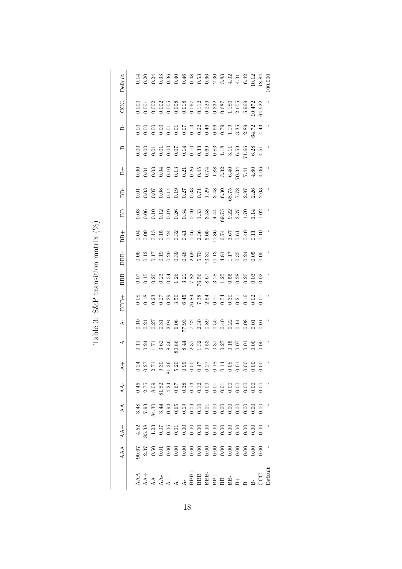
We extract risk-adjusted, forward default probabilities using the model described in Section 2. We do this numerically using a least squares fit in order to enforce the monotonicity of default probabilities for successive ratings categories. The historical rating transition matrix we use to extract the forward default probabilities is shown in Table ??. This matrix is the twelve power of a matrix estimated from monthly transitions in Standard & Poor’s ratings. Given the transition matrix and an assumed recovery rate of 50%, we find the forward default probabilities in each period that best fit the observed spread cross-section.
Figures 6 to 9 show corporate bond forward default probabilities over time for 2- and 5-year maturities and for investment grade and sub-investment grade. For short maturity (2-year) spreads, the time profile of default probabilities mimics that of the spreads themselves as one might expect. For longer (5-year) maturities, the forward default probabilities exhibit dynamics that differ from those of spreads.
4.3 Volatilities and Correlations
Tables 4 and 5 show the volatilities of log forward default probabilities (by rating and maturity) extracted respectively from corporate bond and ABS data. The ABS volatilities are lower for very short maturity (1-year) high grade exposures (AAA and AA) but are higher for longer maturities for any rating and consistently higher for lower ratings. In general, the volatility results suggest striking differences between ABS and corporate bond forward default probability distributions
Table 6 shows the correlations matrix of log forward probability changes by rating for 2-year maturity corporate bonds. The main interest of the table is the evidence it provides for a partitioning of corporate bond risk by credit quality. Entries immediately offthe diagonal, i.e., correlations between forward default probabilities for adjacent ratings, are very high. AAA, AA+ and AA appear closely correlated. However, AA- appears closer to the A+ category than the AA category. Similarly, BBB- is more related to BBB than to BB+. The picture that emerges therefore is one in which the ranges four ranges: (i) AAA to AA, (ii) AA- to BBB-, (iii) BB+ to B-, and (iv) CCC alone, show distinct risk behavior.
The distinctions between the different forms of credit risk is underlined by the fact that in the top right and lower left corners of the correlation matrix, negative correlations may be observed.
Table 7 reports comparable correlation matrix for ABS forward default probabilities. Here the forward default probabilities below BBB have been inferred from the fit of higher rated securities so one cannot draw any conclusions from the lower ratings grades. It appears that BBB is somewhat uncorrelated with the higher grades however.
Tables 8 and 9 show correlations for changes in log forward default probabilities distinguished by maturity. Here, iN ase of corporate bonds (Table 8) the picture is one of smooth decline in correlation as distance in maturity grows. This is consistent with a two factor world in which weight shifts from one factor to the other as maturity increases. In the case of ABSs (Table 9) a similar picture emerges but with a more rapid decline in correlation as maturity grows.
To provide a more formal statistical measure of the number of factors driving risk, Table 10 shows eigenvalues for the correlation matrix in Table 6 and for several sub-matrices. Looking across the whole matrix, the first eigenvalue represents 46% of the eigenvalue sum. Two other eigenvalues are quite large in this case. In the AAA to AA range, the first eigenvalue is 92.3% of the total whereas it is 62.5% in the AA- to BBB- range. The eigenvalues for the correlation matrix by maturity reinforces the impression that there are two dominant factors, one at the short and one at the long end of the term structure.
We performed a similar eigenvalue analysis of the ABS correlation matrices. For the correlation matrix or forward default probabilities by rating, there are three substantial eigenvalues suggesting no simple factor structure. The eigenvalues for the maturity-based correlations suggests a two factor world as the corporate bond case.
4.4 Expected Returns and Risk Premia
Figure 11 shows the time profile (actually plotted against declining maturity) of a AAA forward default probability associated with a particular calendar date (10 years after the start of the sample). While the forward default probabilities should be martingales in the risk neutral measure, they may change over time under the physical probability measure; and indeed this is exactly what we observe in the case depicted in the figure.
To be precise, the log forward default probability declines from -5.9 to about -6.6 over the 4 years of the sample period. In other words, the downward drift in the default probability is of the order of 70% or just under 20% per annum over the first four years of the ten year exposure.
This decline may be interpreted as the decline required to compensate agents for holding claims with spread risk, i.e., it is reflective of the spread-volatility risk premium.
5 Portfolio Value Simulations
Having estimated processes for the forward default probabilities, it is interesting to explore the economic significance of them in a portfolio context. In this section, we therefore report results on a set of simulations we performed on a realistic bond portfolio with and without spread risk and over different horizons.
Characteristics of the bond portfolio we study are provided in Tables 12 and
13. The portfolio is reasonably diversified. It contains 150 exposures and the maximum bond position face value is less than double the average value. The distribution of ratings is reasonably even. The largest parts of the portfolios are around A and the low B range.
The portfolio model used for the simulation corresponds to the ratings based framework described in Section 2 except that correlation between rating transitions is provided by an ordered probit approach like that used in Creditmetrics.
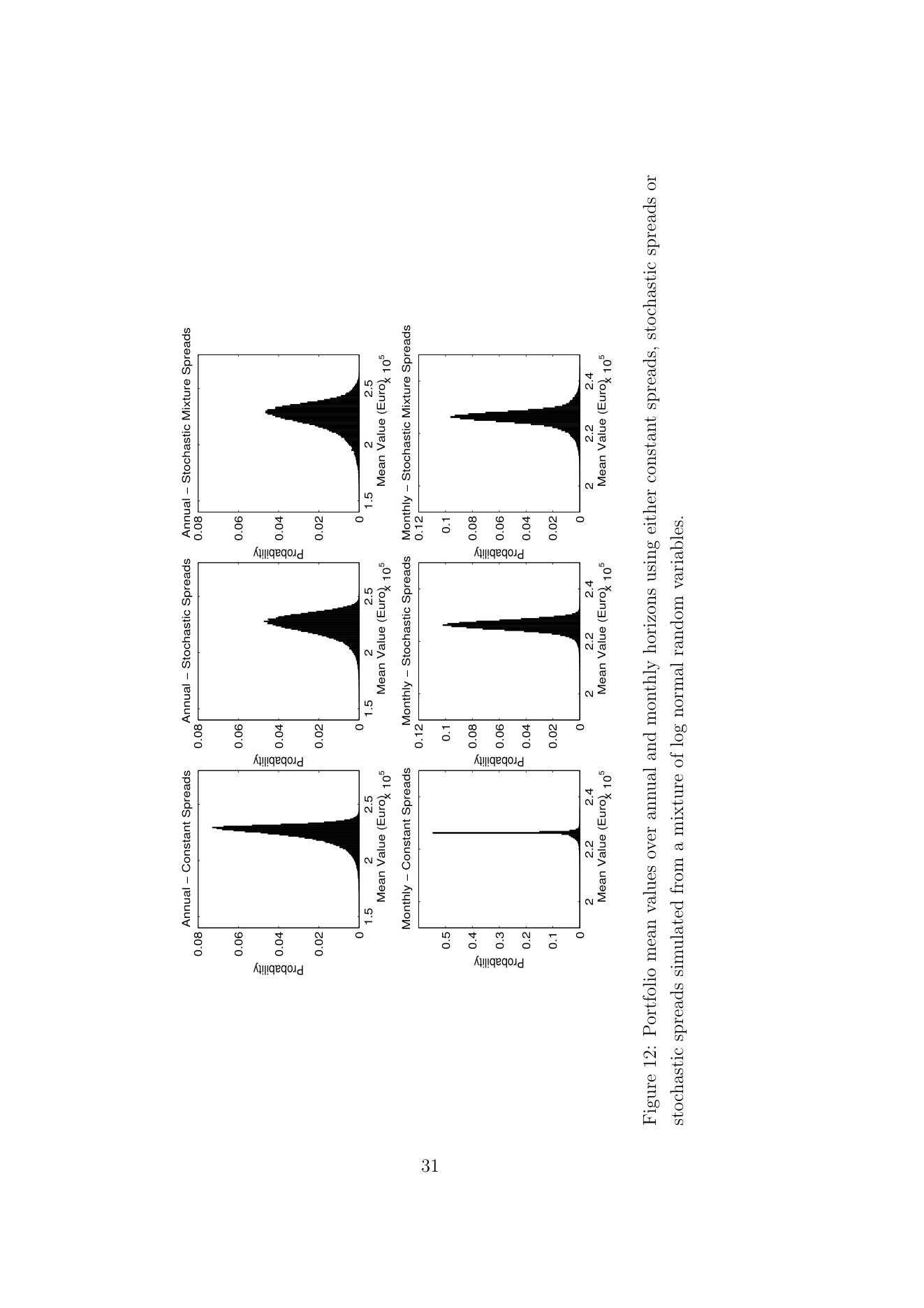
We simulate the portfolio over annual and monthly holding periods assuming (i) constant spreads, (ii) stochastic spreads with Gaussian shocks, and (iii) stochastic spreads with normal mixture shocks. The normal mixture shocks are random draws from two normal distributions. With probabilities 0.7 and 0.3, normals with volatilities of 20% (normal times) and 60% (crisis) are drawn.
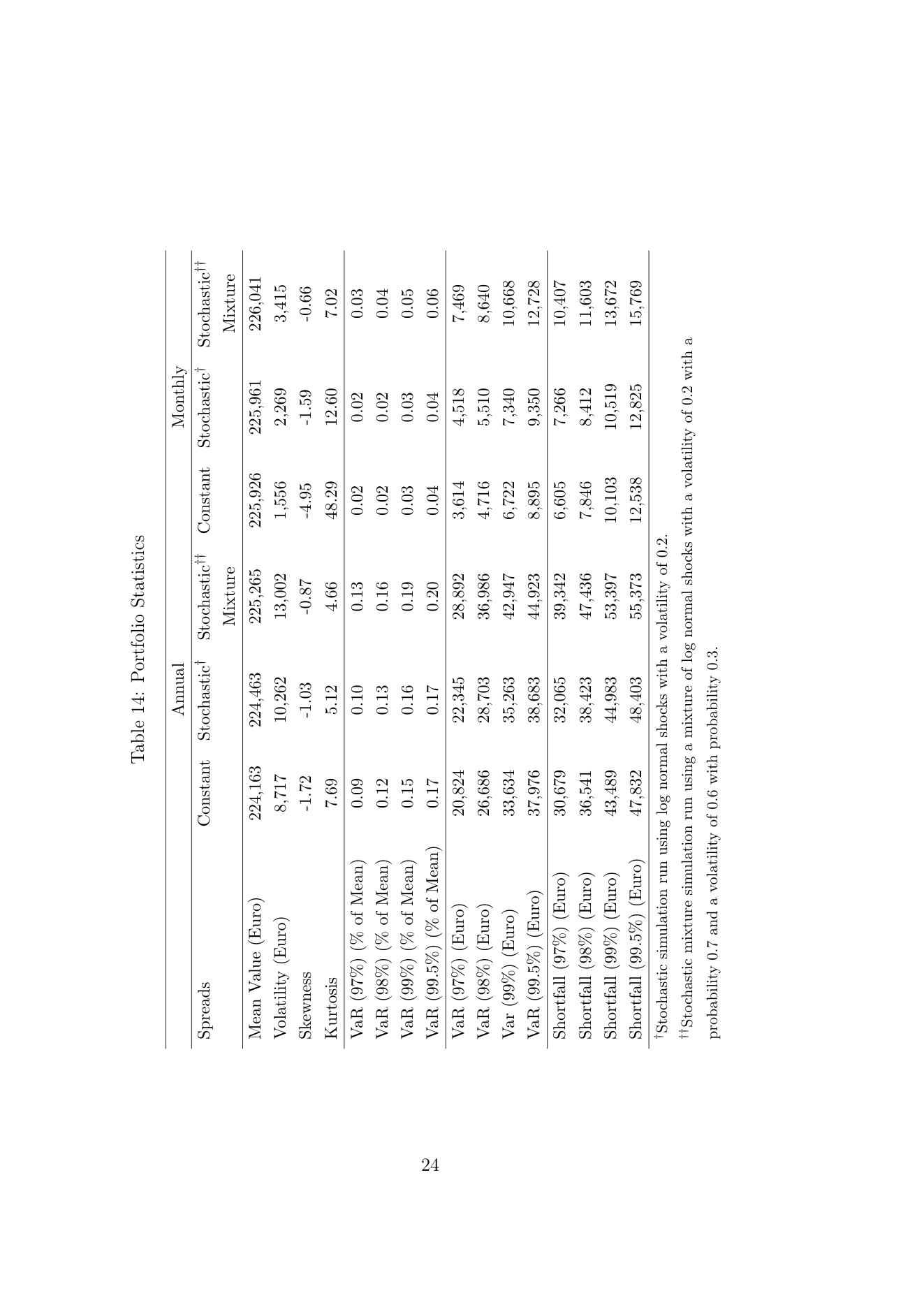
The results of the simulations are shown in Table 14. Portfolio volatilities are highly sensitive to the inclusion of stochastic spreads. VaRs and Expected Shortfall risk measures based on quantiles somewhat out in the tail are less sensitive in the Gaussian case, especially in the case of the longer, 1-year holding period. When shocks are normal-mixture distributed, however, the introduction of stochastic spreads has a substantial impact on risk measures even out in the tail.
6 Conclusion
This paper has empirically investigated corporate bond and ABS spreads using a ratings-based pricing model building on earlier contributions by Jarrow, Lando, and Turnbull (1997) and Kijima and Komoribayashi (1998).
We examine segmentation between credit risk for different maturities and credit qualities by examining volatilities and correlations of forward default probabilities. Our results suggest there is a risk premium on spread risk and we document the fact that it substantially affects portfolio volatility in a realistically parameterized bond portfolio.
7 Appendix A: Derivations
8 Appendix B: Term Structure Fitting Algo- rithm
This appendix briefly describes the techniques for estimating rating-specific defaultable bond term structures devised by Harfush-Pardo, Perraudin, and Taylor (2007). These involve fitting the bond prices using a time-homogeneous, riskadjusted transition matrix restricted to ensure that the right hand column is monotonically increasing in default probability.
A complication is that the use of a risk-adjusted transition matrix implies a discrete time model. So coupon and principal payment dates must be mapped to integer times. More precisely, we map the payment times to the nearest integer number of years. Maintainting the original yield to maturity, we then calculate artificial coupons such that the present value of the bond equals the observed bond price in the data set. Once we have calculated the cash flows and the integer times to payment, we estimate the corporate bond spreads as follows:
1. We start offby guessing some values for the elements of a quarterly transition matrix. We parameterize a tri-diagonal matrix quarterly transition matrix. This implies that the annual transition matrix could have at least four rating migrations to the right and to the left of the diagonal.
2. We then calculate the annual transition matrix, by taking the triangular matrix to the power of 4.
3. We compute that default probabilities at horizons j=1,2,,30 years, which are equal to the right-hand column of the j power of the annual transition matrix.
4. We price the bonds. We assume that the mean recovery rate is 50
5. We calculate the weighted mean of squared price errors. The weights are equal to the time to maturity. Once the optimization routine converges or the maximum number of 2,000 iterations is exceeded, we report the vector of parameters such that the function is minimized. We report spreads on zero coupon bonds for all rating categories and 1 to 30 years to maturity.
References
de Jong, F., and J. Driessen (2006): “Liquidity Risk Premia in Corporate Bond Markets,” mimeo, University of Amsterdam, Amsterdam.
Delianedis, G., and R. Geske (2002): “The Components of Corporate Credit Spreads: Default, Recovery, Tax, Jumps, Liquidity, and Market Factors,” mimeo, Anderson School, UCLA, Los Angeles.
Driessen, J. (2005): “Is Default Event Risk Priced in Corporate Bonds?,” Review of Financial Studies, 18(1), 165–195.
Duffie, D., and K. Singleton (1997): “An Econometric Model of the Term Structure of Interest Rate Swap Yields,” Journal of Finance, 52, 1287–1323.
(1999): “Modeling Term Structure Models of Defaultable Bonds,” Review of Financial Studies, 12, 687–720.
Elton, E. J., M. J. Gruber, D. Agrawal, and C. Mann (2001): “Explaining the Rate Spread on Corporate Bonds,” Journal of Finance, 56(1), 247–277.
Eom, Y., J. Helwege, and J. Huang (2004): “Structural Models of Corporate Bond Pricing: An Empirical Analysis,” Review of Financial Studies, 17(2), 499–544.
Ericsson, J., and O. Renault (2006): “Liquidity and Credit Risk,” Journal of Finance, 61(5), 2219–2259.
Harfush-Pardo, M., W. Perraudin, and A. Taylor (2007): “Estimating Defaultable Bond Spreads by Rating Category,” mimeo, Imperial College, London.
Huang, J.-Z., and M. Huang (2002): “How Much of the Corporate-Treasury Yield Spread is Due to Credit Risk?,” mimeo, Stanford University, Stanford.
Jarrow, R. A., D. Lando, and S. M. Turnbull (1997): “A Markov Model for the Term Structure of Credit Spreads,” Review of Financial Studies, 10, 481–523.
Kijima, M., and K. Komoribayashi (1998): “A Markov Chain Model for Valuing Credit Risk Derivatives,” Journal of Derivatives, 5(Fall), 97–108.
Lando, D. (1998): “On Cox Processes and Credit Risky Securities,” Review of Derivatives Research, 2, 99–120.
Longstaff, F., S. Mithal, and E. Neis (2005): “Corporate Yield Spreads: Default Risk or Liquidity? New Evidence from the Credit Default Swap Market,” Journal of Finance, 60(5), 2213–2253.
Perraudin, W., and A. Taylor (2007): “Liquidity, Bond Market Spreads and Conditional Risk Premia,” mimeo, Imperial College, London.
Table 2: Number of Observation by ABS Type
ABS Sector (%) Total ABS Automobile 31.2 ABS Credit Cards 7.3 ABS Home Equity Loans 40.3 ABS Manufactured Housing 12.9 ABS Miscellaneous ABS 4.7 ABS Utilities 3.6
Table 11: Eigenvalues from correlation matrices for ABS
Correlations across ratings Correlations across maturities Eigenvalue % Total Eigenvalue % Total 1 3.13 44.78 2.96 74.11 2 1.87 26.67 0.85 21.27 3 1.42 20.27 0.18 4.50 4 0.36 5.15 0.00 0.12 5 0.16 2.28 - -
Table 12: Bond Principal and Recovery Assumptions
Average Max. Min. Principal (Euro) 1587 2962 59 Recovery rate (%) 0.48 0.7 0.3 Notes: The portfolio comprises 150 bonds. Recoveries for each bond are assumed to be beta-distributed with a volatility of 0.25.
Table 13: Portfolio Composition
Portfolio Portfolio Fraction (%) Value (%) AAA 0.040 0.040 AA 0.073 0.079 A 0.113 0.117 BBB+ 0.020 0.025 BBB 0.033 0.035 BB+ 0.080 0.076 BB 0.100 0.090 BB- 0.093 0.109 B+ 0.073 0.061 B 0.140 0.138 B- 0.167 0.160 CCC 0.067 0.070 Notes: The total value of the portfolio is Euro 238,035.
AAA AA A BBB
Basis Points
Jun-02 Jan-03 Aug-03 Mar-04 Oct-04 May-05 Dec-05 Jul-06 Trading Date
Figure 2: Investment Grade 5-Year Maturity Corporate Bond Spreads
BBB BB 1600 B CCC
Basis Points
Jun-02 Jan-03 Aug-03 Mar-04 Oct-04 May-05 Dec-05 Jul-06 Trading Date
Figure 4: Sub-Investment Grade 5-Year Maturity Corporate Bond Spreads
AAA AA A BBB
Basis Points
Jun-02 Jan-03 Aug-03 Mar-04 Oct-04 May-05 Dec-05 Jul-06 Trading Date
Figure 5: Investment Grade 2-Year Maturity ABS Spreads
AAA AA A BBB
Basis Points
Jun-02 Jan-03 Aug-03 Mar-04 Oct-04 May-05 Dec-05 Jul-06 Trading Date
Figure 6: Forward Default Probabilities for Investment Grade 2-Year Corporate
AAA AA A BBB
Basis Points
Jun-02 Jan-03 Aug-03 Mar-04 Oct-04 May-05 Dec-05 Jul-06 Trading Date
Figure 8: Forward Default Probabilities for Sub-Investment Grade 2-Year Cor-
BBB BB B CCC
Basis Points
Jun-02 Jan-03 Aug-03 Mar-04 Oct-04 May-05 Dec-05 Jul-06 Trading Date
Figure 10: Forward Default Probabilities for 2-Year Maturity ABS (Recovery
Years to Maturity 10.00 9.58 9.17 8.75 8.33 7.92 7.50 7.08 6.67 6.25 -5.20
-5.40
-5.60
-5.80
-6.00
-6.20
-6.40
-6.60
-6.80 Log of Forward Default Probabilities
-7.00
Figure 11: Constant-Calendar-Date Forward Default Probabilities for AAA Cor-
| Years % | Observations |
|---|---|
| 1 | 27.0 |
| 2 | 24.8 |
| 3 | 18.0 |
| 4 | 9.7 |
| 5 | 6.7 |
| 6 | 4.3 |
| 7 | 2.7 |
| 8 | 1.4 |
| 9 | 2.2 |
| 10 | 1.1 |
| 10+ | 2.0 |
| AAA | AA | A | BBB | BB | B | CCC | |
|---|---|---|---|---|---|---|---|
| 1Y | 34.7 | 19.1 | 10.9 | 7.0 | 13.5 | 18.9 | 16.6 |
| 3Y | 10.2 | 8.0 | 7.6 | 6.3 | 14.2 | 18.6 | 18.1 |
| 5Y | 5.9 | 6.5 | 6.7 | 5.9 | 14.4 | 19.3 | 20.0 |
| 7Y | 5.2 | 5.8 | 6.3 | 7.1 | 15.6 | 20.3 | 21.5 |
| 10Y | 6.1 | 6.9 | 7.4 | 9.1 | 18.2 | 21.8 | 22.6 |
| 15Y | 8.2 | 8.8 | 9.7 | 10.1 | 23.4 | 24.9 | 22.8 |
| 20Y | 10.6 | 11.1 | 11.5 | 11.8 | 28.3 | 28.3 | 17.6 |
| AAA | AA | A | BBB | |
|---|---|---|---|---|
| 1Y | 16.5 | 11.1 | 10.7 | 24.5 |
| 2Y | 13.2 | 9.2 | 9.5 | 22.7 |
| 3Y | 13.8 | 11.8 | 10.4 | 18.2 |
| 4Y | 15.2 | 20.1 | 18.1 | 17.6 |

| maturity | ABS (%) | |||||
|---|---|---|---|---|---|---|
| AAA | AA | A | BBB | BB | B | CCC |
| AAA 100.0 | 61.6 | 71.0 | 7.8 | 13.6 | 30.0 | 30.0 |
| AA 61.6 | 100.0 | 93.9 | 46.1 | 21.8 | 8.7 | 4.0 |
| 71.0 | 93.9 | 100.0 | 44.0 | 21.3 | 16.0 | 13.9 |
| BBB 7.8 | 46.1 | 44.0 | 100.0 | 70.5 | 12.0 | -13.1 |
| BB 13.6 | 21.8 | 21.3 | 70.5 | 100.0 | 61.8 | 22.0 |
| 30.0 | 8.7 | 16.0 | 12.0 | 61.8 | 100.0 | 87.2 |
| CCC 30.0 | 4.0 | 13.9 | -13.1 | 22.0 | 87.2 | 100.0 |
| 1Y | 2Y | 3Y | 4Y | 5Y | 6Y | 7Y | 8Y | 9Y | 10Y | |
|---|---|---|---|---|---|---|---|---|---|---|
| 1Y | 100.0 | 80.2 | 53.7 | 31.4 | 30.3 | 25.6 | 18.7 | 8.1 | -2.1 | -12.5 |
| 2Y | 80.2 | 100.0 | 81.4 | 47.7 | 39.3 | 28.2 | 19.0 | 8.8 | -0.3 | -9.1 |
| 3Y | 53.7 | 81.4 | 100.0 | 85.3 | 70.7 | 52.0 | 39.3 | 31.4 | 25.9 | 18.5 |
| 4Y | 31.4 | 47.7 | 85.3 | 100.0 | 93.1 | 75.6 | 62.0 | 54.5 | 49.8 | 43.1 |
| 5Y | 30.3 | 39.3 | 70.7 | 93.1 | 100.0 | 92.7 | 81.9 | 72.4 | 64.3 | 54.2 |
| 6Y | 25.6 | 28.2 | 52.0 | 75.6 | 92.7 | 100.0 | 96.7 | 89.3 | 80.0 | 68.6 |
| 7Y | 18.7 | 19.0 | 39.3 | 62.0 | 81.9 | 96.7 | 100.0 | 97.2 | 90.0 | 80.1 |
| 8Y | 8.1 | 8.8 | 31.4 | 54.5 | 72.4 | 89.3 | 97.2 | 100.0 | 97.3 | 90.6 |
| 9Y | -2.1 | -0.3 | 25.9 | 49.8 | 64.3 | 80.0 | 90.0 | 97.3 | 100.0 | 96.8 |
| 10Y | -12.5 | -9.1 | 18.5 | 43.1 | 54.2 | 68.6 | 80.1 | 90.6 | 96.8 | 100.0 |
| 1Y | 2Y | 3Y | 4Y | |
|---|---|---|---|---|
| 1Y | 100.0 | 53.4 | 32.3 | 25.8 |
| 2Y | 53.4 | 100.0 | 93.4 | 76.8 |
| 3Y | 32.3 | 93.4 | 100.0 | 92.5 |
| 4Y | 25.8 | 76.8 | 92.5 | 100.0 |
| Correlations | across | ratings Correlations | across | maturities | |
|---|---|---|---|---|---|
| Eigenvalue | % | Total | Eigenvalue | % Total | |
| 1 | 7.82 | 46.0 | 20.23 | 67.4 | |
| 2 | 2.91 | 17.1 | 6.19 | 20.6 | |
| 3 | 2.03 | 11.9 | 1.46 | 4.9 | |
| 4 | 1.33 | 7.9 | 1.01 | 3.4 | |
| 5 | 0.87 | 5.1 | 0.68 | 2.3 | |
| Correlations | AAA | to AA Correlations | 1Y-4Y | maturities | |
| Eigenvalue | % | Total | Eigenvalue | % Total | |
| 1 | 2.77 | 92.3 | 2.92 | 73.0 | |
| 2 | 0.20 | 6.5 | 0.84 | 21.1 | |
| 3 | 0.03 | 1.2 | 0.21 | 5.3 | |
| 4 | - | - | 0.02 | 0.5 | |
| Correlations | AA- to | BBB- Correlations | 5Y-10Y | maturities | |
| Eigenvalue | % | Total | Eigenvalue | % Total | |
| 1 | 4.37 | 62.5 | 5.19 | 86.5 | |
| 2 | 1.30 | 18.6 | 0.67 | 11.1 | |
| 3 | 0.11 | 1.6 | 0.12 | 2.0 | |
| 4 | 0.62 | 8.9 | 0.01 | 0.2 | |
| 5 | 0.03 | 0.5 | 0.00 | 0.1 |
Notes
∗To contact the authors, please email mariam.harfush-pardo@riskcontrollimited.com, rlamb@ic.ac.uk or wperraudin@ic.ac.uk