Rating Correlations and Macro Stress Testing

1 Introduction

This study brings together two highly topical issues: credit correlation and conditional modeling of credit quality dynamics. On the first of these issues, the credit crunch has highlighted the need to improve understanding of correlation in bond and loan markets. Such correlations influence the value of structured products such as Asset Backed Securities (ABS) and Collateralized Debt Obligations (CDO). They are also a key input to credit portfolio models which may be used to assess the riskiness of a given financial institution or of the banking system as a whole.

Agency credit ratings are a widely used measure of credit quality in bond and loan markets. Ratings agencies such as Moody’s and Standard and Poor’s assign letter grade ratings to credit instruments according to the likelihood that they will default in the future. Historical data is available on the evolution of these ratings over time for a large number of obligors. Furthermore, the capital accord Basel II encourages banks to use internal or external rating system to calculate capital requirement for their credit portfolio. Rating based models, thus, have become an industry standard approach in credit risk management. As a result, it is important to study the credit market correlations implicit in historical ratings histories.

On the second issue, conditional modeling of credit quality dynamics, this is an important input to bank stress testing. The recent crisis has increased interest among regulators and financial institutions in the use of risk management approaches that rely more on the evaluation and study of stress scenarios or stress tests of different kinds. (See, for example, Borio, Drehmann, and Tsatsaronis (2014) and Acharya, Engle, and Pierret (2014).) One may think of stress testing as risk analysis of portfolio outcomes conditional on particular adverse scenarios. As such, stress testing is a natural complement to more traditional risk measurement (such as the calculation of Value at Risk (VaR) or Expected Shortfall (ES)) which is generally performed on an unconditional basis.

Conditional modeling of ratings dynamics are also central to the modeling efforts in which many banks are engaged to meet the requirements of the IFRS 9 accounting standard. Under this standard, banks must forecast their expected losses conditional on the current state of the macroeconomic cycle. This requires the development of coherent approaches to Point-in-Time (PIT) and Through-the-Cycle (TTC) ratings (bank’s internal ratings frameworks are TTC whereas IFRS 9 requires a PIT viewpoint) and then rigorous approaches for estimating future expected losses.

In this paper, we study correlations or dependency between ratings changes for borrowers from different sectors. We do this both unconditionally and conditional on shocks to macro economic variables. Our approach therefore suggests ways of benchmarking or parameterizing standard unconditional VaR or ES analysis while also showing how one may perform macroeconomic stress tests, both within a single unified framework.

A variety of techniques for estimating ratings change distributions have been proposed in the literature. Most studies have focused on default correlations (i.e., binary default/no-default events) but the techniques proposed are equally applicable to trinomial events (up-grade/down-grade/no change in rating), or to fully multinomial events (such as ratings changes). In particular, Gordy (2000) proposes a method to calibration asset correlation by matching the moment of conditional default probability. Servigny and Renault (2002a) estimate correlations from default data using a moment-based estimator. They estimate the correlation between default and non-default events within given time periods and then transform this into the correlation between Gaussian latent variables. Frey and McNeil (2003) perform moment-based and Maximum Likelihood estimations of default correlations. McNeil and Wendin (2006) and McNeil and Wendin

(2007) estimate correlations from default and ratings transitions using Bayesian techniques.

Other authors who have analyzed the correlations implicit in credit default data include Chernih, Vanduffel, and Henrard (2006), Chernih, Vanduffel, and Henrard (2006), Das, Freed, Geng, and Kapadia (2006), Dulmann and Scheule (2003), Frey, McNeil, and Nyfeler (2001), Gagliardini and Gourieroux (2005a) and Gagliardini (2005b), Gordy and Heitfield (2002), Kijima, Komoribayashi, and Suzuki (2002), Koopman, Lucas, and Klaassen (2005), Lamb and Perraudin (2008), Lopez (2004), Pitts (2004) and Schwaab, Koopman, and Lucas (2017).

In this paper, we use historical data on Moody’s ratings to estimate correlations for latent variables driving credit ratings both within and between sectors. We suppose that ratings changes (intrinsically discrete phenomena) are driven by continuously distributed latent variables. These latent variables are presumed to be correlated and Gaussian. In performing our estimations, we allow for the fact that the latent variables driving the ratings are not directly observed. We extend the above (unconditional) framework by supposing that the common sector factors driving ratings changes have an observable component that we identify with innovations in GDP. We then repeat our ML estimations but conditional on historically observed GDP shocks.

The fact that our analysis supplies conditional distributions of the evolution of portfolio credit risk implies that our approach may be used in stress testing. Stress testing conditional on macroeconomic scenarios, commonly termed macro stress testing, has become an important component of the battery of stress tests that bank regulators now require of the institutions they supervise. Macro stress testing has also been performed by regulators as part of the system-wide stress tests that they themselves have implemented, post the crisis, to assess systemic risk in different countries’ banking markets.

Berkowitz (1999), Kupiec (1998), Lopez (2005) and Schachter (2001) discuss how stress testing may be used in ways that complement and are more or less integrated with VaR analysis. CGFS (2001), CGFS (2005) and CGFS (2000) present survey information and best practice guidelines on stress testing in financial firms. Blaschke, Jones, Majnoni, and Peria (2001) and Elsinger, Lehar, and Summer (2005) discuss how stress testing may be used to assess the stability of banking systems as a whole. Building on Pesaran, Schuermann, and Weiner (2004), Pesaran, Schuermann, Treutler, and Weiner (2006) present techniques for implementing macro stress testing for a banking portfolio.

The paper is organized as follows. Section 2 presents the modeling approach. Section 3 presents estimation results. Section 4 shows simulations of the model. Section 5 concludes. Numeric integration and statistic inference techniques employed in this research are described in the Appendix.

2 The Model for Credit Rating Correlation

2.1 A Latent Variable Model

In this section, we present the approach of two-step maximum likelihood estimations for credit correlation embedded in ratings data. The credit correlations within a sector are initially estimated, then the credit correlation between each pair of sectors are obtained in the second estimation. We also extend this two-step approach to conditional analysis in which macro stress testing can be conducted.

Here we present a multivariate, latent variable model of credit rating migrations. The framework is based on assumptions similar to those employed in rating-based portfolio credit risk models (see, for example, Gupton, Finger, and Bhatia (1997)). In brief, the approach supposes that for each obligor in a given period a standard Gaussian random

(latent) variable is drawn and that the change in the obligor’s rating is determined by the interval of the real line in which the latent variable realization falls. Furthermore, this latent variable is a linear combination of a systematic risk factor and an idiosyncratic risk factor. Exposures are correlated since they share systematic risk factor. So dependency between ratings changes for different obligors is introduced by supposing that the latent variables are joint Gaussian. Li (2000) shows that the Credit Metric factor model is essentially a Gaussian Copula model.

More formally, consider a portfolio consisting of n = 1, 2, .., N obligors from i = 1, 2, .., K industries. Let rn,t denote the rating at time t of the nth obligor. Let I(n) denote the nth obligor’s industry which we assume to be constant over time. Suppose there are J ratings categories (including the default state) and that rn,t takes values in the set of integers: {1, 2, · · · , J}.[1]

Suppose that changes in the rating of the nth obligor are driven by a latent variable

p1 − ρnϵn,t, (2.1) xn,t = √ρnfI(n),t +

where

≡ is the industry factor for obligor n realized at date t fI(n),t ≡ is a constant industry factor loading of the nth obligor ρn ≡ is the nth obligor′s idiosyncratic shock at time t . (2.2) ϵn,t

Suppose that both fI(n) and ϵn,t are independent standard normal variables. It follows that the latent variable xn,t is also standard normal.

Given these assumptions, the obligors in a given industry have a single common risk factor. For two industries, i and j, the corresponding factors, fi,t and fj,t, are assumed to have a correlation coefficient denoted ρi,j.

In addition to industry classification, this model allows us to group obligors into homogenous buckets such as according to geographic region or initial rating. An other advantage, as mentioned in Gordy and Heitfield (2002), is that we only need to keep track of one risk factor per bucket. So we can think of industry factor fI(n) as a summarizing effect on obligors in this industry. So ρn is the sensitivity of obligors to the industryspecific common risk factor.

Suppose that the rating at date t of obligor n is determined by its rating in the prior period and the realization of the latent variable xn,t. For each initial, non-default rating category, i = 2, 3, . . . , J, zi,k(n) for k = 1, 2, . . . , J − 1, denote a set of J − 1 cutoffpoints. If rn−[1] = i, then, let:

rn = 1, if xn < zi,(n[1]);

. if z(n) rn = j, i,j−1 < xn < zi,j(n);

Assuming the value of these cutoffpoints and that latent variables are distributed as standard normal random variables, the probabilities of rating migrations are:

= Φ(z(n) Pr [rn = 1] i,[1] ), = Φ(z(n) (2.3) Pr [rn = j] i,j ) − Φ(zi,j(n)−[1]), = 1 − Φ(z(n) Pr [rn = J] i,J−[1]).

Here, Φ(.) is the standard normal probability distribution function.

The expressions in equation (2.3) are unconditional transition probabilities. Conditional on the industry factor fI(n), and initial rating i, one may show that the probabilities of one-step-ahead ratings are:

! zi,(n1) −√ρnfI(n) Pr rn = 1|fI(n) = Φ , √1 − ρn ! ! zi,j(n) −√ρnfI(n) zi,j(n)−1 −√ρnfI(n) Pr rn = j|fI(n) = Φ − Φ , (2.4) p1 − ρI(n) √1 − ρn ! zi,J(n)−1 −√ρnfI(n) Pr rn = J|fI(n) = 1 − Φ . √1 − ρn

The statistical model we employ here contains Random Effects resulting from com- If the common factor were observable, then the model would mon risk factor fI(n). reduce to the Ordered Probit Model with the link function being the standard normal distribution function. This type of model belongs to a larger class called Generalized Linear Mixed Model (GLMM) as pointed out by (Frey and McNeil (2003)). The advantage of using GLMM is that it can handle continuous covariate as well as polytomous variables such as credit ratings. Greene (2011) provides a good introduction to this subject.

In what follows, we shall assume that the ratings of all individual obligors within a sector have identical distributions. In particular, we suppose a constant ρn for any exposure, n, within a given sector, k, and that the transition probabilities are also identical for exposures in a sector. With a slight abuse of notation, we may write the factor loading for the nth exposure in the kth sector as ρk where k = I(n). Similarly, the cutoffpoints may be written as zi,j(k) for exposures within the kth sector. An appealing feature of the above model is that correlation is implicitly built into the structure of the latent variables in (2.1). Both the inter and intra industry correlations can be derived from it. For example, the correlation between the latent variables for two obligors from sector k is ρk, while the correlation between the latent variables of obligors from sectors i and k is √ρiρkρi,k, where ρi,k is the inter-sector correlation between industry factors fi and fk. In general, if ρ is a diagonal matrix of intra sector correlations, and ρf is a matrix of inter sector correlations, then the unconditional latent variable (at obligor level) correlation matrix is p Σ = ρ′ρf√ρ (2.5)

We now turn to how one may estimate the intra industry and inter industry correlations by Maximum Likelihood Estimation (MLE).

2.2 Maximum Likelihood Estimation for Correlation

There exist different approaches in the credit risk literature to estimating credit correlation based on ratings data. It is common to employ moment-based estimation approaches as in Servigny and Renault (2002b). However, empirical studies suggest these approaches leads to downward biased correlation estimates (see Gordy and Heitfield (2002) and Gagliardini and Gourieroux (2005a)). Maximum Likelihood Estimation may have better small sample properties. However, there are technical challenges in calculating the likelihood function because one must integrate over the common factor. In some cases, the integration is of high dimension. McNeil and Wendin (2007) propose Bayesian techniques (including the Gibbs Sampler) which avoids the problems of high dimensional integration and permits the use of priors. Here, we propose a simpler Maximum Likelihood approach involving multi-step estimations.

We assume though out that time is discrete with a time step equal to one year. To estimate intra- and inter-industry correlation matrix, two Maximum Likelihood Estimations may be performed. In such a two-step approach, the results of the first set of estimations yield inputs to the second set of estimations. Let Nij(k)(t) denote the number obligors in industry k rated i at date t which migrate to j one year later. The data on ratings migrations in a given period and for a given industry may be arranged into a (J − 1) × J count matrix,

h i N(k)(t) = Nij(k)(t) .

If all rating changes were independent, the likelihood for the count data would consist of the product of a set of probabilities of moving from one rating to another where these probabilities would be taken powers equal to the number of obligors observed to make transitions between particular pairs of ratings. However, in the model described above, rating changes are correlated through the correlation of the latent variables which drive them since these latent variables contain a common risk factor. The rating changes are, therefore, only independent if one conditions on the common factor. Calculating the likelihood then involves forming the product of probabilities taken to the relevant powers conditional on the common factor and then integrating over this factor.

Rather than using all possible ratings changes, we simplify the problem by restricting attention to observations of (i) upgrades, (ii) downgrades and (iii) observations in which ratings do not change. Major rating agencies such as Moody’s and Standard & Poor’s monitor and publish information on historical defaults as well as upgrade and downgrade rates. Hamilton and Cantor (2004) argues that downgrades and upgrades are taken seriously by banks in pricing credit instruments and thus affect credit spreads.

We denote the number of ratings upgrades, no changes and downgrades for obligors in sector k in period t with initial rating i as:

J X NiU(k)(t) = Nij(k)(t), j=i+1 NiN(k)(t) = Nii(k)(t), i−1 X NiD(k)(t) = Nij(k)(t). j=1

The corresponding conditional probabilities of upgrade, no change and downgrade are:

! Zi,i(k) −√ρkfk PiU(k)(t) = 1 − Φ , √1 − ρk ! ! Zi,i(k) −√ρkfk Zi,i(k−) 1 −√ρkfk PiN(k)(t) = Φ − Φ , (2.6) √1 − ρk √1 − ρk ! Zi,i(k−) 1 −√ρkfk PiD(k)(t) = Φ . √1 − ρk

Here, zi,j(k) is the jth cutoffpoint of sector k for the rating migration from initial rating i to terminal rating j. And time index for fi is omitted for simplicity. For industry k and initial rating i, the conditional probability of observing all rating migrations in year t are independent. Hence, the joint likelihood is

h i J NiU(k)(t) + N (iNk)(t) + N (iDk)(t) ! h Y PiU(k)(t)NiU(k)(t)PiN(k)(t)NiN(k)(t)PiD(k)(t)NiD(k)(t)i N(k) i=2 iU (t)! × N (iNk)(t)! × N (iDk)(t)! J Y = A(ik)(t)L(ik)(fk, t; ρk). i=2 Here, h i NiU(k)(t) + N (iNk)(t) + N (iDk)(t) ! A(ik)(t) = , NiU(k)(t)! × N (iNk)(t)! × N (iDk)(t)! and L(jk)(fk, t; ρk) represents the product of upgrade, no-change and downgrade probabilities. To calculate the unconditional probability, one must integrate over the common factor, fk. Suppose for sector k, a series of rating migration count matrices, N(k)(t), are observed for periods t = 1, . . . , T . The unconditional log likelihood of all rating migrations may be written as:

T J Z X Y = log A(k) Lk(ρk) i (t)L(ik)(fk, t; ρk) dΦ(fk) R t=1 i=2 T J Z X Y ∝ log L(ik)(fk, t; ρk) dΦ(fk). (2.7) R t=1 i=2 Here, the constant terms A(ik) are omitted since they play no role in estimation and Φ(.) is the standard normal cumulative distribution function.

The above likelihood function is similar to what have been presented in Gordy and Heitfield (2002) and Frey and McNeil (2003). But in their work they only consider binary default/non-default events. Here, we employ a multinomial probit mixture model.

For a pair of sectors k = 1, 2, conditional on factors f[1] and f[2], the probability of observing all rating migrations in both industries is

2 J Y Y A(ik)(t)L(ik)(fk, t; ρk). i=2 k=1 To calculate the unconditional probabilities for rating migrations in both industries, one must integrate over both factors f[1] and f[2].

Suppose for sector k = 1, 2, two series of rating migration count matrices N(1)(t) and N(2)(t) are observable for years t = 1, . . . , T . The unconditional log-likelihood of all rating migrations in both sectors is:

T 2 J Z Z X Y Y = log A(k) L[12](ρ[1], ρ[2], ρ[12]) i (t)L(ik)(fk, t, ρk) dΦ[2] (f[1], f[2]; ρ[12]) R R t=1 k=1 i=2 T 2 J Z Z X Y Y ∝ log L(ik)(fk, t, ρk) dΦ[2] (f[1], f[2]; ρ[12]) . (2.8) R R t=1 k=1 i=2

Here, constant terms A(ik) are omitted and Φ[2] is the standard bivariate normal cumulative distribution function with correlation ρ[12].

To summarize, when deriving the likelihood function, we use the property of conditional independence so that the joint likelihood is the product of all probabilities, and then integrate over the common factor(s) to remove the conditioning. For an univariate industry, conditional on the industry factor fi, rating migrations are independent within the industry. For a pair of industries, conditional on both industry factors f[1] and f[2], rating migrations in both industries are independent.

Again, for simplicity, we estimate the parameters sequentially. Initially, we estimate intra-industry correlations for each industry by using likelihood function (2.7), i.e., es- ∀k = 1, · · · , I. Then, for any pair of industries, given the intra industry timate ρk, correlations estimated in the first MLE, we use likelihood function (2.8) to estimate the inter-industry correlation. This two-step approach has the major advantage that each Maximum Likelihood Estimation (MLE) only requires that one maximize the likelihood over a single scalar parameter for intra-industry correlations and over two dimensions for inter-industry correlations.

If we estimated the parameters for all the sectors together, the aggregated likelihood function would be similar to that employed in McNeil and Wendin (2006). The requirement of integrating over multiple dimensions would make Maximum Likelihood scarcely feasible in that case, however. Including autocorrelation as McNeil and Wendin

(2006) would further exacerbate the problem. McNeil and Wendin (2006) and McNeil and Wendin (2007) circumvent these difficulties by using Bayesian techniques. Our sequential estimation approach makes Maximum Likelihood feasible in a multi-industry setting, reducing the integration to at most two dimensions. Specifically, we employ

Gauss Hermite Quadrature as described in Burden and Faires (2010). Appendix provides details.

2.3 Conditional Latent Variable Model

In the unconditional model described above, the latent variable is described by equa- Now, tion (2.1) in which the common factor for sector k at time t is denoted fk,t. suppose that fk,t is a weighted sum of an economy-wide common factor, ft, and an industry-specific shock, gk,t, i.e.,

p p (2.9) fk,t = βkft + 1 − βk gk,t.

Here, ft and gk,t are independent, standard, normally-distributed random variables satisfying E(gigj) = ρ(ijg), and βk is a constant factor loading. The inter-industry factor correlation (the correlation between fi and fj) may be expressed in matrix notation as:

pβ′β + p(1 − β)′(1 − β) · ρ(g). (2.10)

Here, · denotes element-by-element multiplication, β is a column vector made up of elements βi, ρ(g) is the correlation matrix of g, and 1 is a column vector of ones with the same dimensions as β.

The inclusion of an observable common factor ft introduces what in statistical language is referred to as fixed effects. The observed variable introduces a time varying effect from overall economic conditions, influencing obligors in different sectors. Nickell, Perraudin, and Varotto (2000), Bangia, Diebold, Kronimus, Schagen, and Schuermann (2002), Hu, Kiesel, and Perraudin (2002) and Wei (2003) and many others have found evidence that rating migrations are influenced by observable macroeconomic variables. Hence, rating migrations do not conform to a time-homogenous Markov Chain. Unfortunately, observed variables are unable to explain all the dynamics in rating migrations, so the unobservable common factor gk,t (specific to a sector) should be retained in the model.

Since the economy-wide factor, ft, is observable, one may again employ the approach described above for the unconditional model to derive likelihood functions for estimating both intra- and inter-industry correlations. We denote this specification with the associated likelihoods as the conditional model, reflecting the fact that the economy-wide factor, ft, is treated as given. The log likelihood functions in the intra- and inter-industry cases, see equations (2.7) and (2.8), are almost unchanged except that

(i) the conditional probability, becomes

! p Zi,i(k) −√ρkβkf − ρk(1 − βk)gk P˜iU(k)(t) = 1 − Φ , √1 − ρk p ! Zi,i(k) −√ρkβkf − ρk(1 − βk)gk P˜iN(k)(t) = Φ (2.11) √1 − ρk ! p Zi,i(k−)[1] −√ρkβkf − ρk(1 − βk)gk −Φ , √1 − ρk ! p Zi,i(k−)[1] −√ρkβkf − ρk(1 − βk)gk P˜iD(k)(t) = Φ . √1 − ρk

Here, the time index for factors gk and f is omitted for simplicity.

(ii) In the unconditional model, it is necessary to calculate the likelihood function conditional on the common factor, fk. However, in the conditional model, fk may be split into the observable component ft and the unobservable industry shock gk. So, in this case, one must calculate the likelihood function conditional on gk.

To summarize, the intra-industry conditional log-likelihood for all rating migrations for sector k is:

T J Z X Y ∝ log L(k) (2.12) Lk(ρk, βk) i (gk, t; ρk, βk)dΦ(gk). R t=1 i=2

Here, L(ik)(gk, t; ρk, βk) = P˜ (iUk)(t)NiU(k)(t)P˜iN(k)(t)NiN(k)(t)P˜iD(k)(t)NiD(k)(t).

Similarly the inter-industry conditional log-likelihood for all rating migrations for two industries denoted k = 1, 2 is:

∝ (2.13) L[12](ρ([12]g), ρ[1], ρ[2], β[1], β[2]) T 2 J Z Z X log Y Y L(ik)(gk, t; ρk, βk)dΦ g[1], g[2]; ρ([12]g) . R R t=1 k=1 j=2

Again, we shall estimate these parameters sequentially. In particular, there are three consecutive Maximum Likelihood estimations. First, we estimate the intra-industry correlations ρk using likelihood function (2.7) in unconditional model. Next given intra industry correlation obtained in the first maximum likelihood estimation, estimate economy wide factor loading βk using likelihood function (2.12). And finally given the results in the first and the second maximum likelihood estimation, estimate correlation for inter sector shock ρ(ijg) using likelihood function (2.13). The advantage of this 3-step estimation is similar to that of in the unconditional model. That is in each estimation only one parameter is iterated and the joint distribution is consistent with its breakdown margins.

3 Results

3.1 Data

To implement the model, we use Moody’s issuer ratings data for US-domiciled issuers from the start of 1990 to mid 2010. We combine the Moody’s industry classification with the North American Industry Classification System (NAICS) to divide the data into 15 sectors. See Moody’s (2010) and NAIC (2007) for detailed information on their respective industry classifications. The sectors we employ and associated acronyms are listed below.

1. Oil and Gas: OG.

2. Mining: Coal and Metal: Mn.

3. Real Estate: RE.

4. Information: Inf.

5. Transportation: Trp.

6. Heavy Engineering and Technology: HET.

7. Consumer Goods: CG

8. Medical and Pharmaceutical: Md.

9. Banking: Bk.

10. General Manufacturing: GM.

11. Public Administration: PA.

12. Telecom: Tel.

13. Utility: Ut.

14. Agriculture: Ag.

15. Business Service: BS.

Table 1 provides data on the number of observations available for each sector year by year. One may observe that Banking and Heavy Engineering and Technology are the two sectors for which most data is available, accounting for more than a half of the total observations. Relatively few observations are available for other sectors. Among them, Agriculture has the fewest observations.

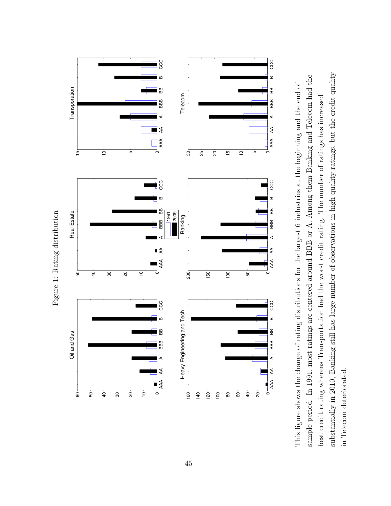
Data frequencies by initial rating at the start and end of the sample period are shown in Figure 1. The un-shaded bar represents ratings observations in 1991 while the black bar stands for ratings observations available for 2010. In 1991, the distribution is centered on BBB or A. Among them, Banking and Telecom observations tend to have the highest credit ratings whereas Transportation obligors have the lowest credit ratings. The number of rated obligors has increased substantially over the sample period. The Banking sector still has the largest number of observations in high quality ratings. But the credit quality of Telecom obligors has somewhat deteriorated.

The estimation of correlation parameters we perform is based on ratings up-grades, down-grades and observations for which ratings are unchanged. So, it makes sense to inspect these three types of data directly as well as using them in the estimation routines.

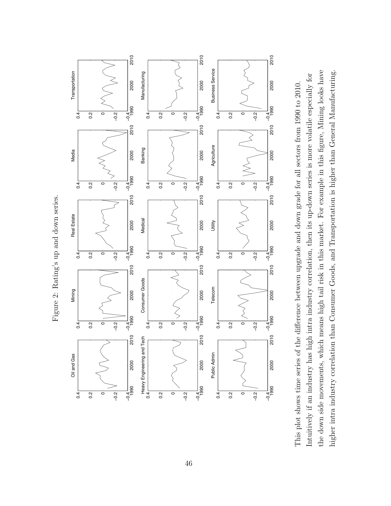
Figure 2 plots the difference between up- and down-grades for all sectors across all sample periods. If an industry’s time series is more volatile and exhibits large fluctuations, then one would expect this industry to be highly correlated in the sense that the intra-industry correlation parameter will be large in magnitude. In other words, if correlation is high, the chances of observing more up grades than down grades (or vice versa) in particular periods is high. From the figure, one may observe that Heavy Engineering & Technology, Consumer Goods and Utility have lower intra-industry correlation, whereas Mining, Media and Transportation have higher intra industry correlation.

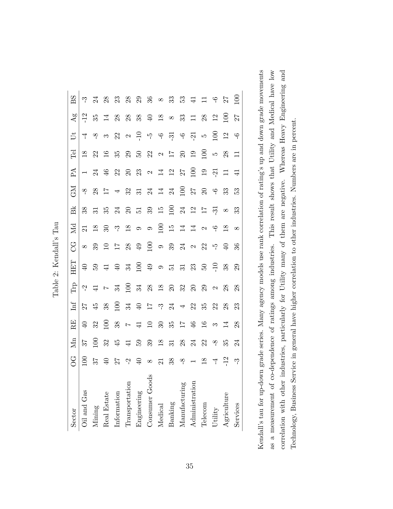
It is common in credit market research to use rank correlation of up- and down-grade ratings movements to measure the co-dependence of ratings changes across industries. For example Akhavein, Kocagil, and Neugebauer (2005) infer asset correlation from Kendall’s Tau by observed rating upward, downward and no-movement. Table 2 calculates Kendall’s Tau for the up-grade minus down-grade series. The table shows that Utility and Medical have lower intra-sector correlation with other industries. In the case of Utility, many are actually negative. Heavy Engineering, Technology, and Business Service, on the other hand, tend to have higher intra-sector correlations than other sectors.

3.2 Estimation for Unconditional Model

The sequential estimation approach we adopt implies that need only optimize likelihood functions over a single dimension. In particular, we initially estimate intra-industry correlation, ρi, sector by sector, maximizing the log likelihood of upgrades, downgrades and no-movements. This likelihood is shown in equation (2.7). After estimating the intra-industry correlations, we estimate inter-industry correlations, ρik, for each pair of industries. If there are N industries, this implies there are N(N[2]−1) inter-industry correlation parameters to estimate. We maximize the likelihood shown in equation (2.8).

Intra-industry correlations based on 20 years of historical data for US-domiciled corporate ratings are shown in Table 3. In this table, one may see that the results are broadly consistent with the data depicted in Figure 2. Those industries with volatile up-down series tend to possess higher intra-industry correlations. Clearly, correlation estimates vary across different sectors, the range of magnitude being from 5% to 20%. In the Basel II document of BCBS (2005), asset correlations for sovereigns, banks and corporate are in principle to take value between 12% to 24%. Our results show correlations slightly lower than the Basel values. In this our study resembles other empirical studies, see Frey and McNeil (2003), Akhavein, Kocagil, and Neugebauer (2005) and McNeil and Wendin (2006). In other words, the Basel II correlation values are more conservative than those suggested by historical data. Hansen, Vuuren, and Ramadurai

(2008) argues that this conservatism is appropriate given the global scope of Basel II and the need to accommodate, for example, differences across banks in risk factor sensitivity, concentration risk and model risk.

The industries that exhibit low correlations are Consumer Goods, Utility and Heavy Engineering & Technology. Mining, Real Estate and Transportation have the highest intra-industry correlations. Standard errors are presented in parentheses in Table 3[2].

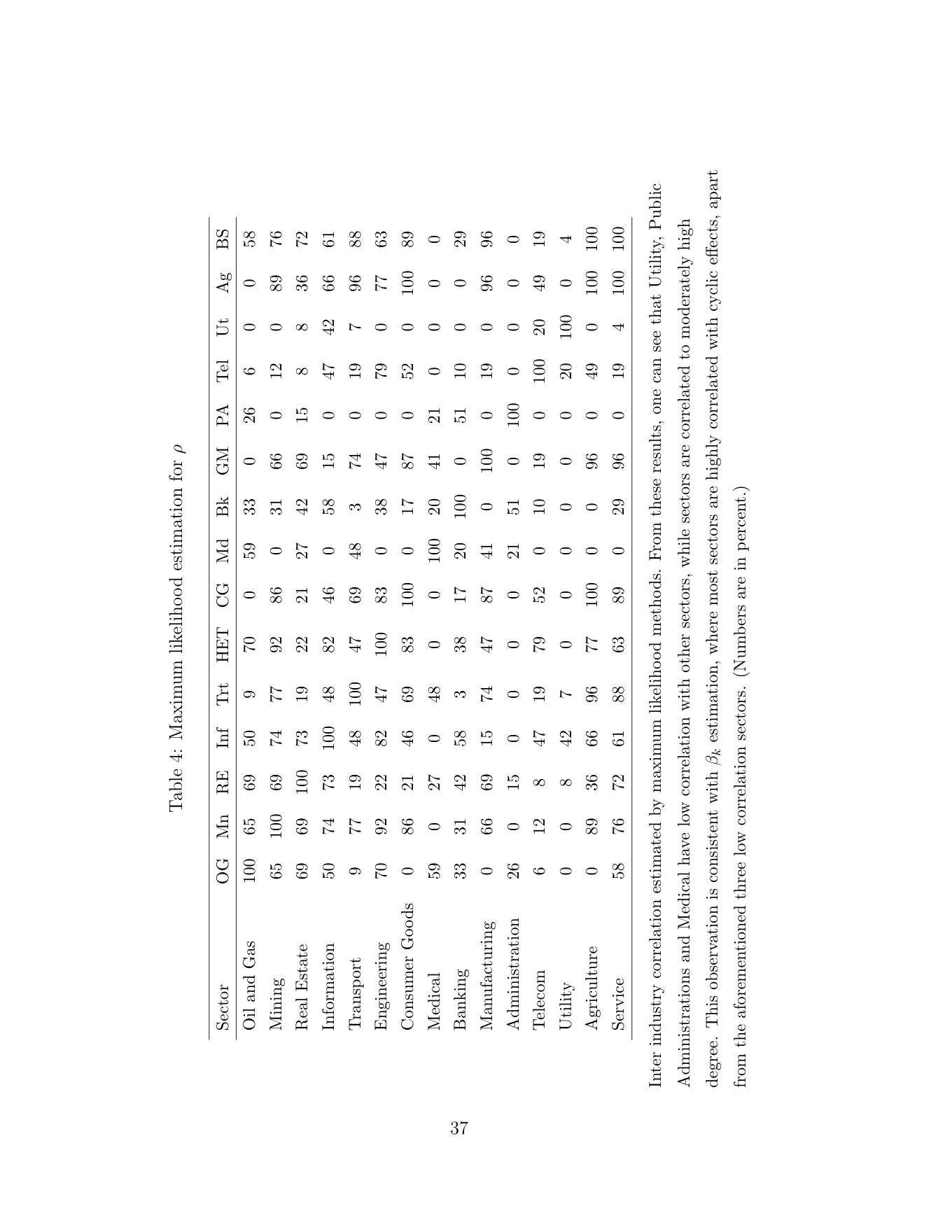
The results on inter-industry correlation estimations, ρf, are shown in Table 4. We will discuss the inter-industry correlation matrix in the next section when we provide estimation results for the conditional model.

3.3 Estimation for Conditional Model

In the conditional model, the log likelihood function (see equation (2.12) ) may be maximized over ρi and βi using data on the observed economy-wide factor and the ratings changes for the industry. One may either estimate ρi and βi simultaneously or employ estimates ρi from unconditional model using equation (2.7) and then substitute these into the conditional model. The results obtained from the two methods turn out to be very similar. A similar approach may be applied to estimating the pairwise interindustry estimation. Having estimated the intra-industry parameters, ρ and β may be substituted into equation(2.13) to estimate ρ(g).

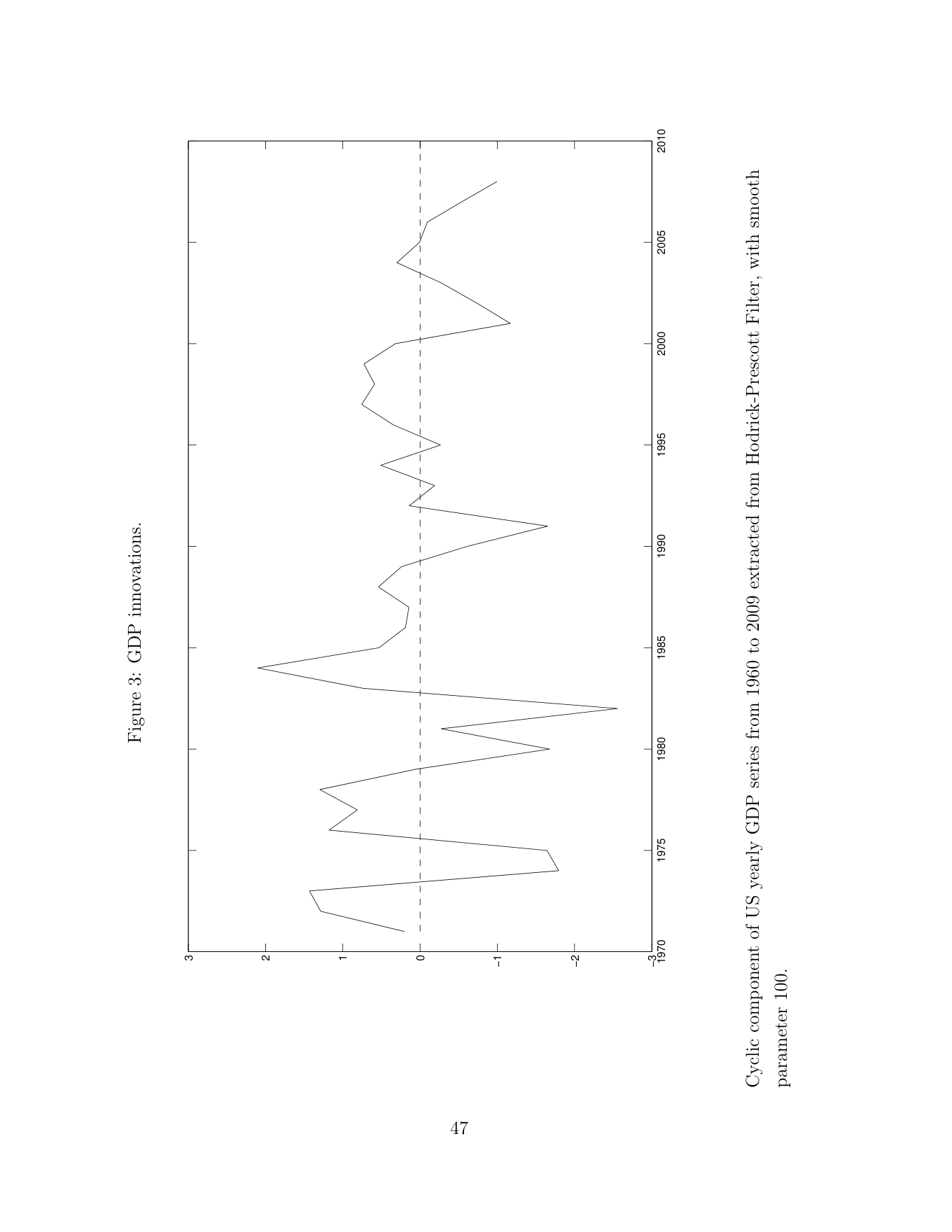
The observable macroeconomic factor we employ consists of innovations to GDP as measured by deviations from trend based on the Hodrick-Prescott filter, For more information, see Hodrick and Prescott (1997) and Leser (1961). This filter consists of a technique of deducing a trend in a macroeconomic time series. See the Appendix for details. Deviations from the trend may be regarded as innovations. In the conditional model, these innovations are assumed to equal the economy wide factor f(t). This factor, by assumption, must have unit variance and a zero mean. So we normalize the process accordingly. see Figure 3 for extracted GDP innovations. We perform a Ljung-Box Qtest for serial correlation. The results, contained in Table 12, show that one cannot reject at a 1% significance level the null hypothesis that the process is serially uncorrelated.

The parameter estimates for β and its standard errors are presented in Table 3. The parameter βi is the sensitivity of the risk factor driving latent variable in the ith sector to the business cycle as measured by the Hodrick-Prescott-filtered GDP series. Most values are positive apart from Medical, General Manufacturing and Public Administration which are close to zero. Given the sign conventions of the model, positive parameters imply, as one would intuitively expect, that increases in GDP are associated with credit rating upgrades. The degree of cyclical sensitivity evident for the different sectors is reasonably convincing. Information, and Business Service have the highest beta values, while Real Estate, Transportation and Agriculture have moderately high beta values. The Medical, Utility, Public Administration and Manufacturing sectors have low betas with values less that 20%. Of them, 3 have betas close to zero. Thus, more that half of the sectors have high sensitivity to GDP shocks.

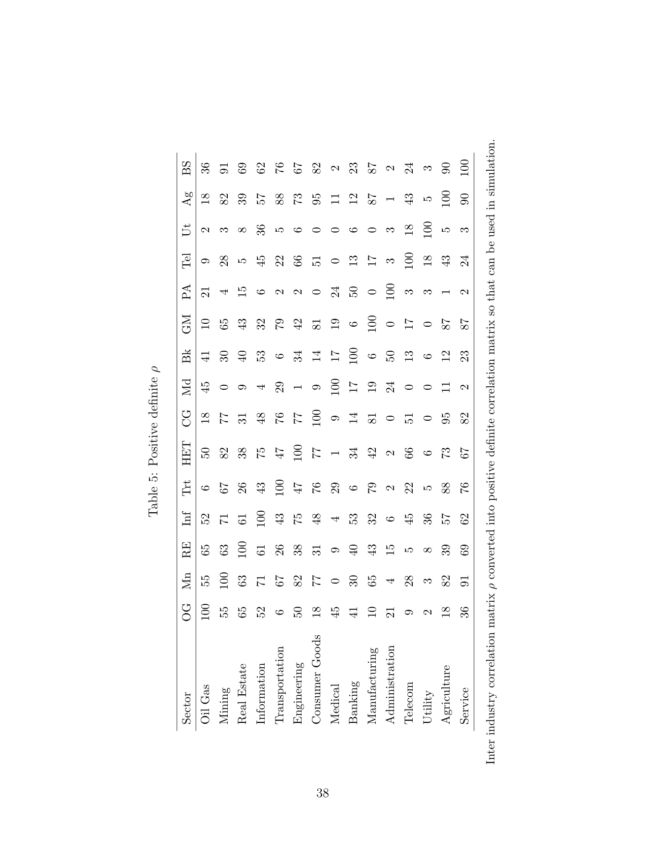
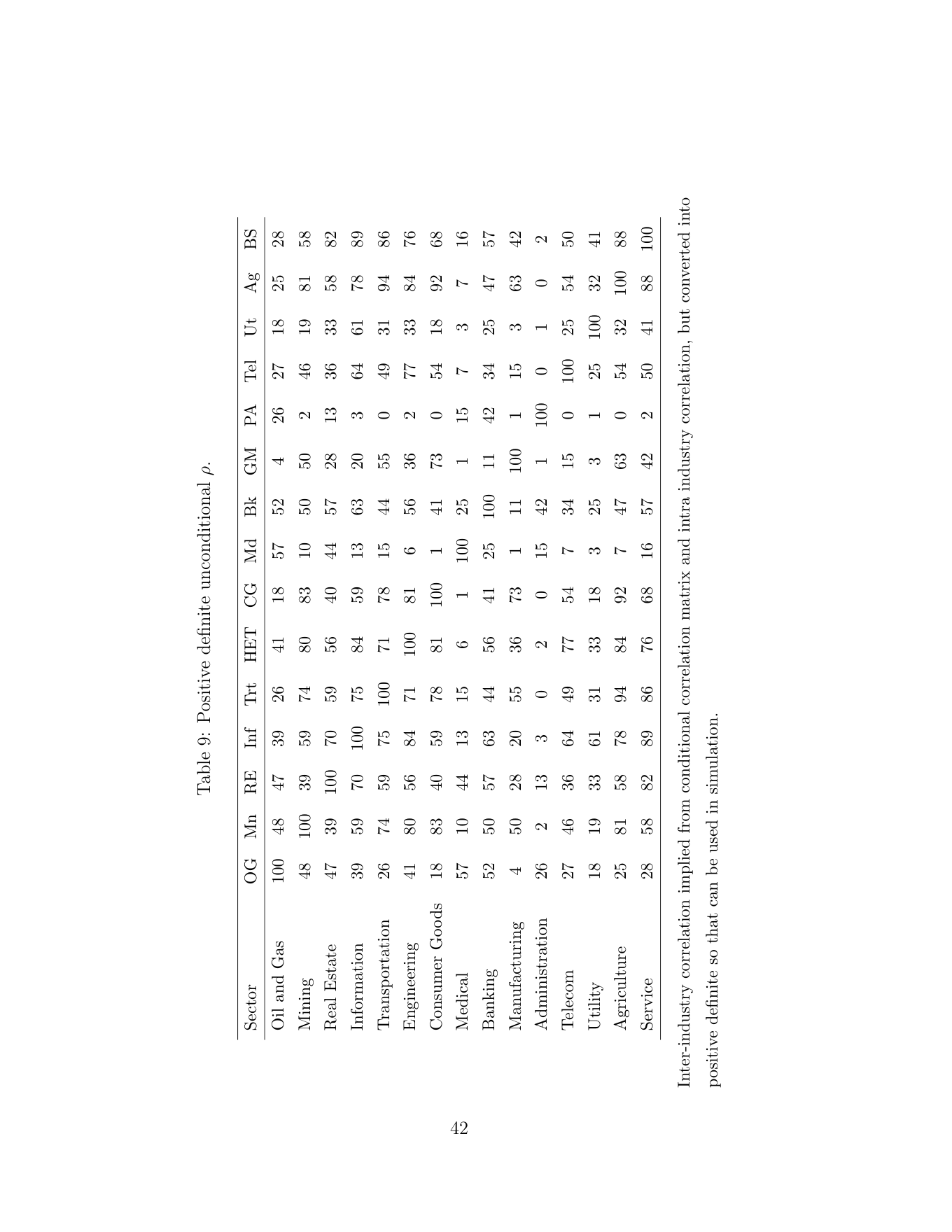
The inter-industry correlation matrix is presented in Table 4. For its associated positive-definite matrix, see Table 5. One can use this correlation matrix to calculate the (obligor-level) latent variable correlation matrix by using equation (2.5). The obligor-level correlations across different sectors are substantially lower than the intrasector correlations, as one might expect. By using S&P’s ratings data, McNeil and Wendin (2006) estimate 8.7% of intra-industry correlations on average and 2.6% for inter-industry correlations. Our results show the average of inter-industry correlations is around 4%, with the highest value being 16%. The correlations estimated by Hansen, Vuuren, and Ramadurai (2008) using Fitch ratings data around 3%-4% with the highest value being around 10.6%.

From these tables, one may see that Utility, Public Administrations and Medical have low correlations with other sectors, while the Business Services, Agriculture, Mining, and Heavy Engineering and Technology sectors tend to have high correlations with other sectors. Other sectors are correlated to a moderately high degree. These findings are consistent with the estimation results already reported for βk.

One may compare the MLE estimates with the rank correlation results shown in with other sectors, whereas Heavy Engineering and Technology, Business Services have higher correlations with other sectors. These results are broadly consistent with the MLE estimation results.

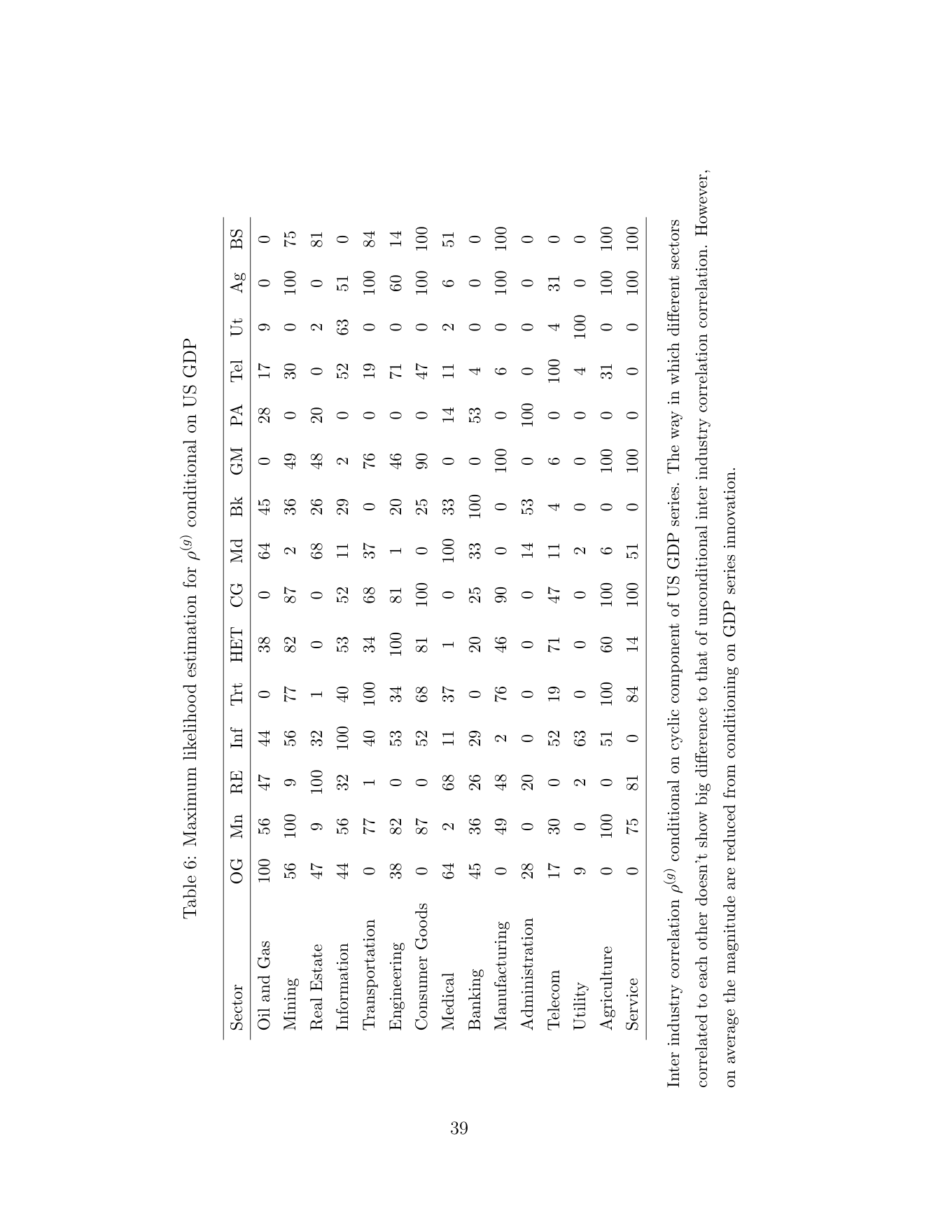
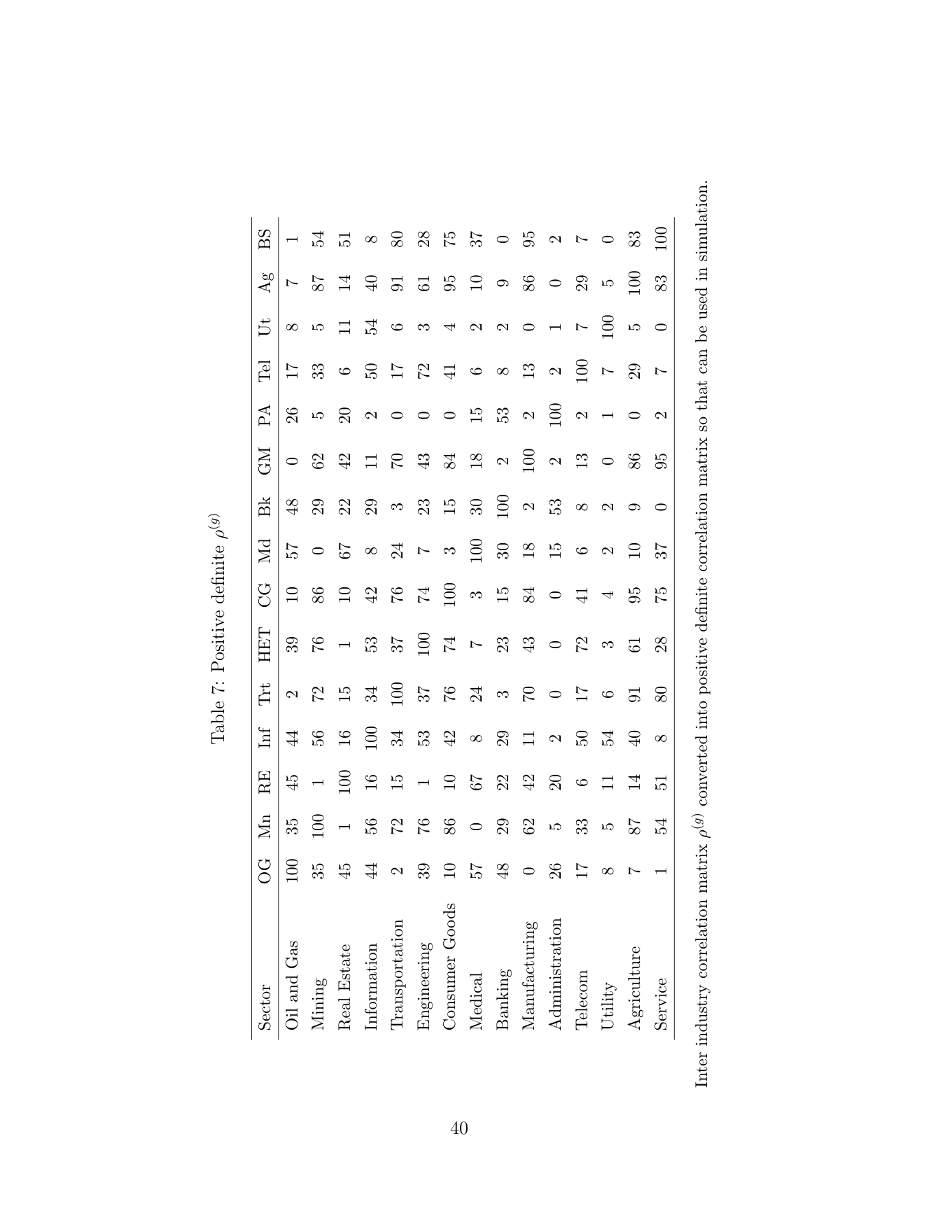
Conditional on the common cyclical factor, the inter-industry correlation matrix ρg is presented in Table 6. The associated positive-definite matrix is reported in Table 7. See the Appendix for a discussion of how the correlation matrices are transformed to ensure positive definiteness. The pattern of correlation across different sectors is little affected by enforcing such positive definiteness. It is interesting to compare the conditional inter-industry correlation matrix ρ(g) with the unconditional inter-industry correlation matrix in Table 4. Of the entries in the matrices, 77% of the scalar conditional correlations are smaller than their unconditional counterparts.

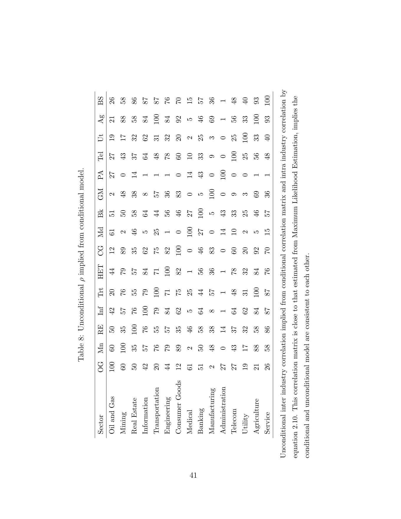
The implied inter-industry correlation matrix, ρf, calculated from equation (2.10), is presented in Table 8. Comparing this table with the estimated inter-industry correlation matrix in Table 4, one may note that the two inter-industry correlation matrices are broadly similar, which testifies to the consistency of the conditional and unconditional approaches.

4 Simulation Tests

4.1 Reverse Test

This section consists of two parts. In the first, we evaluate our estimation techniques using Monte Carlo analysis. Specifically, we generate data for hypothesized, multisector portfolios with predetermined initial ratings. Given the parameters for both intra- and inter-sector correlations, we simulate ratings changes in the portfolio. Finally we estimate the correlation parameters using the simulated data. In the second part of the section, we conduct stress testing analysis on the hypothesized portfolio. We then calculate the distribution of the portfolio value conditional on the worst GDP shock that occurs within our sample period.

The aforementioned models involve intensive numerical calculations. For example, to evaluate the likelihood function numerically requires integration techniques using Hermite Gauss Quadrature. It is helpful, therefore, to evaluate the performance of the algorithms we employ. To this effect, we simulate ratings yearly time series for two industries. In constructing the simulated dataset, we suppose there are 20×7 companies with 1/7th allocated to each of the rating categories from AAA to CCC. We then use the simulated data to estimate both intra- and inter-industry correlations.

To test the correlation model, two cases are examined. In the first case, we test the general performance of the model with low and high intra-sector correlations and short and long sample periods. In particular, the following correlation values are employed: ρ[1] = 0.05 and ρ[1] = 0.3 with sample periods of 30 years, 60 years and 100 years. Estimates of intra-industry correlations for these different cases are provided in Table 10.

From Table 10, one can observe that the means of the estimated correlation are very close to the true values in all cases. As the sample size grows, the standard deviation of the mean estimates declines. The model produces more accurate results when the correlation is low, but when correlation is at a high level, the approach tends slightly to underestimate the true value. Similar results were found by Gordy and Heitfield (2002) in their simulation analyses. This bias may reflect bias in the Maximum Likelihood estimation approach or numerical issues associated with the limited precision a computer can achieve. Specifically, in this model, when the common factor is very large, the conditional probabilities employed within the likelihood are very small. The problem may be alleviated by (i) scaling the probability, (ii) and using more points in the Hermite Gauss Quadrature.

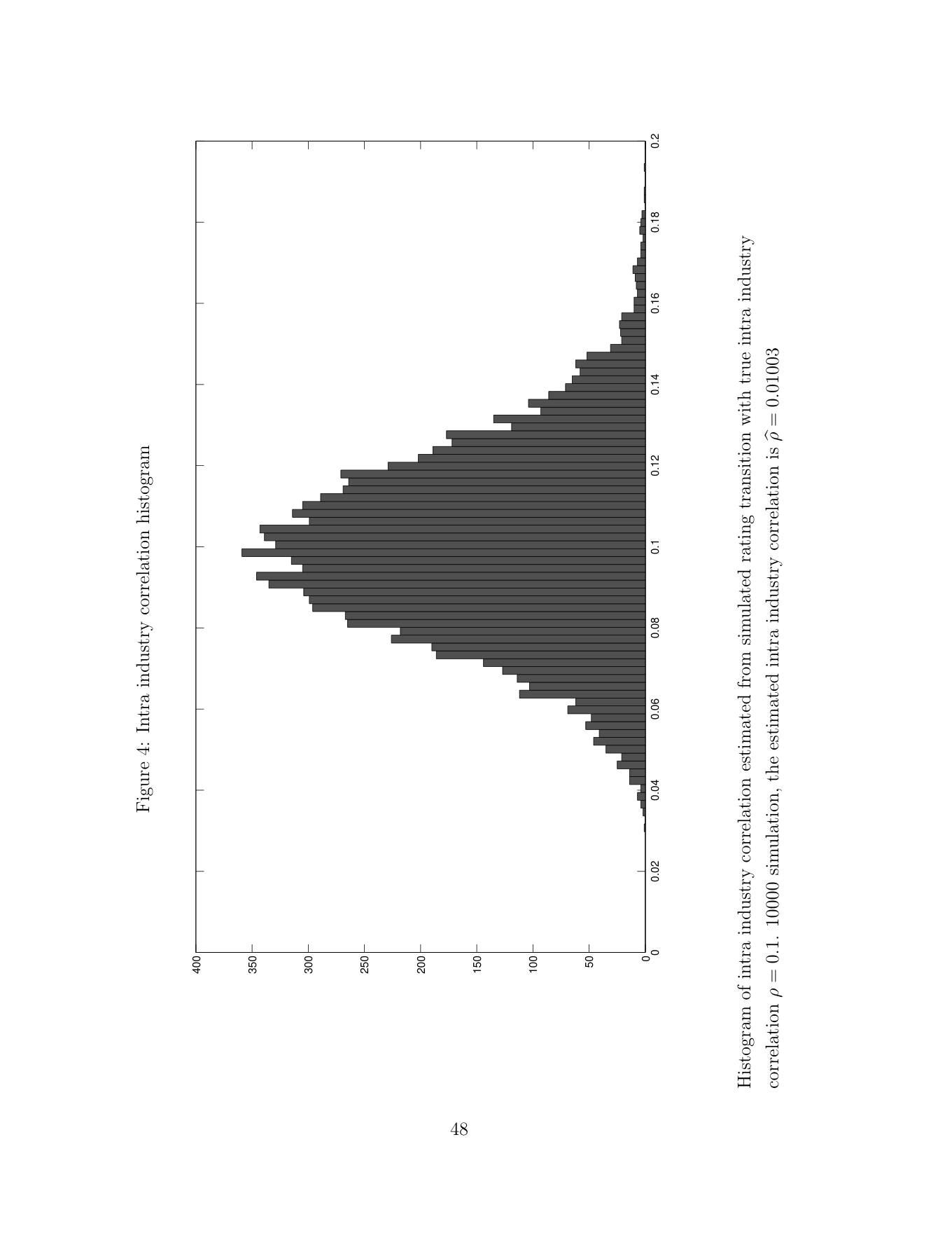
We then perform a second simulation exercise with a single intra-industry correlation value of 10% and 10,000 replications. The results are shown as a histogram in Figure 4. The the mean of the estimates is equal to 10.03% which is very close to its true value.

For inter-industry correlation we test the model by high, median and low correlation, in particular ρ = 0.1, 0.5, 0.8. In this case, we perform 1,000 simulations with 30 and 60 years of simulated data. Table 11 presents results suggesting the model is able to handle large inter-correlation well. With small a sample size of 30 years of data, inter-industry correlation values are negatively biased when the true value is small. When the sample size is increased to 60 years, the bias is reduced substantially.

In general, we believe the above analyzes demonstrate the robustness of the approach and the correctness of the implementation.

4.2 Stress Test

Basel II requires that bank perform stress testing to assess the sensitivity of their portfolios to extreme market conditions. Some stress testing involves formulating scenarios expressed directly in terms of macroeconomic scenarios (see BCBS (2005)). One may observe from historical data that during periods of low macroeconomic activity, defaults tend to cluster. So when performing stress testing, some may propose to boost correlation so as to differentiate normal market conditions. The problem is that we do not know to what degree we should boost correlation for stress testing purposes. A more formal approach such as one based on our conditional model then seems appealing.

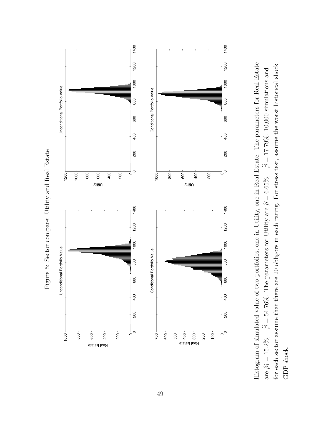
In our conditional framework, different sectors with different level of correlations respond to the stressed conditioning variable in to differing degrees. As an example, we formulate here stress testing for two portfolios each comprising 100 bonds in a single sector. The two sectors on which we focus are: Real Estate and Utility. The bonds are evenly distributed across the coarse, non-default ratings categories. Each bon has a face value of 100 and a maturity of two years. Using the parameters estimated in previous sections, we perform two simulation exercises each with 10,000 replications. In the first exercise, we compute the distribution of the value of each portfolios using the unconditional model. Next, conditional on the worst historical GDP shock in Figure 3 (which equals a shock of to -2.56%), we recompute the value of both portfolios using conditional model.

The upper row in Figure 5 plots the unconditional density of the simulated value for both portfolios as a histogram. The intra-sector correlations are 15.2% for Real Estate and 6.65% for Utility. As shown in the figure, the unconditional means of the portfolios are similar, reflecting the fact that the exposures in the two portfolios have the same ratings, par-values and maturities. In particular, the mean value for both Real Estate and Utility is 918. However, since the intra-sector correlation for Real Estate is much higher than Utility, the distribution of Real Estate is more spread out with a a longer left-hand tail. The one percent quantile for the Real Estate portfolio distribution is 748 which is significantly lower than the value of 811 for Utility.

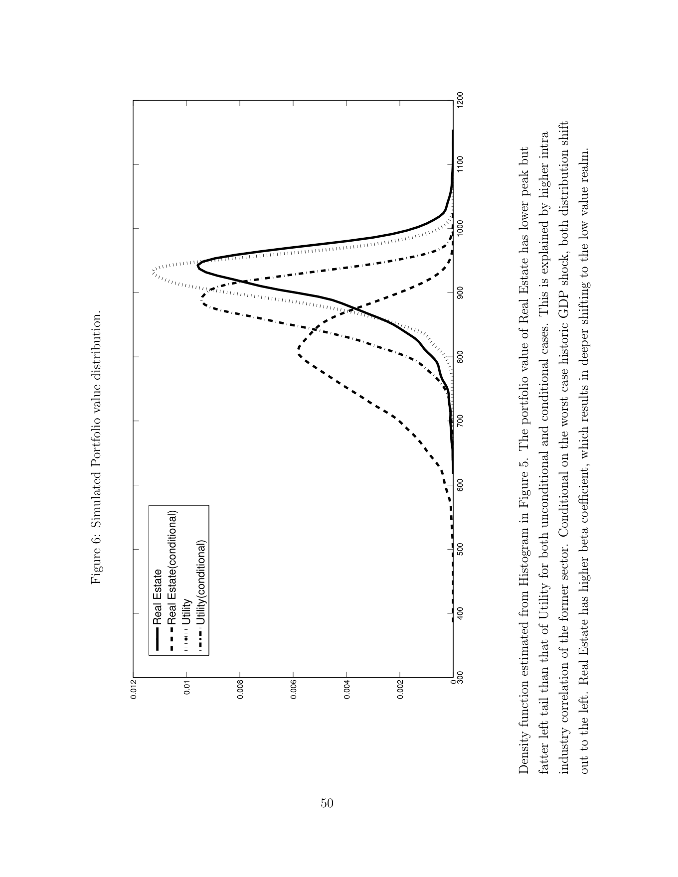
The bottom row in Figure 5 conditional densities for the simulated values of both portfolios in the form of histograms. The factor loading parameter β represents the sensitivity to general economic conditions. For exposures in Real Estimate, the estimated beta coefficient is equal to 54.76%, whereas for Utility it is equal to 17.79%. Conditional on the worst case historic GDP shock, we can see that both distributions shift to the left. For Utility, the conditional mean falls to 879, a reduction of 39 compared to the unconditional mean of 918. The one percent quantile falls to 755, a reduction of 56 from 811 . For Real Estate, the conditional mean value of portfolio falls to 793, a drop of 125, while the one percent quantile declines to 602, a reduction of 146 from 748. In response to the worst GDP shock in the sample period, Real Estate shows a deeper drop in value and expansion in the left tail. This shift shift is also clearly apparent in Figure 6.

In general the stress test results show that a portfolio of Utility bonds may perform reasonably even during extreme macroeconomic condition (reflecting the fact that its intra-sector correlation and beta coefficients are low). In contrast, a portfolio of Real Estate bonds is likely to perform poorly in macroeconomic downturns reflecting the fact that the correlation and macroeconomic sensitivity parameters are relatively high.

5 Conclusion

Quantities such as default probability, recovery rates and correlation play decisive roles in both credit pricing and risk management by banks in the context either of their banking or trading books. In contrast to other parameters, correlations in credit risk analysis are harder to measure and, even if measurable, notoriously unstable.

This paper attempts to capture credit correlations using Moody’s rating data from 1990 to 2010. We estimate both intra- and inter-industry correlations using Maximum Likelihood estimations with numeric integration. The analysis is implemented both unconditionally and conditionally. The conditional approach permits one to implement macro stress testing in which the credit quality of a portfolio is simulated conditional on a hypothesized future path of real GDP innovations.

The main results of the analysis are as follows.

1. Intra- and inter-industry correlations vary systematically across industry sectors. For example, intra-industry correlations range from about 5% to 21% in the unconditional model. Similar results are found in the conditional model, with beta coefficients for GDP innovations varying across sectors. These results suggest the importance of distinguishing between sectors in credit risk modeling and capital management.

2. Conditional on the macroeconomic factor we investigate, GDP innovations, most correlations between sectors tend to decrease. This suggests the majority of sectors exhibit a cyclical pattern, with ratings moving on average with the broad economic cycle.

3. However, the conditional analysis also reflects differing sensitivities across different sector. We illustrate this by showing that a portfolio of non-cyclical industries such as Utility exposures is much less sensitive to adverse GDP shocks than a comparable portfolio of Real Estate bonds.

This paper makes several contributions to the current literature. First, most empirical analysis of correlation has focussed on on default correlation rather than ratings transitions. Here, we implement a multinomial approach applied to ratings changes including defaults. Second, we develop a conditional version of our empirical analysis and show how this can be applied in macro stress testing. Third, Maximum Likelihood appears to be difficult in higher dimensional, multi-sector cases. Other studies have proposed simulation-based Maximum Likelihood methods or Bayesian techniques. Here, we show the effectiveness of multi-step Maximum Likelihood estimation, which as we demonstrate is tractable and transparent and yields comprehensible and intuitive estimates.

Appendix

A1 Numeric Integration

When computing likelihood functions in the context of intra-industry correlation estimation, one must evaluate a one-dimensional integral with respect to the common factor. When estimating inter-industry correlation by Maximum Likelihood, one must calculate a double integral with respect to two correlated common factors. In performing integrations, we employ Gauss Hermite Quadrature. Here, we explain how we apply the Gauss Hermite Quadrature approach to bivariate cases.

Integrating a function, g(x), with respect to a standard normal density is straightforward in that one evaluates:

n Z X g(x)f(x) = wixi. R i=1

Here, f(x) is the density function of the standard normal variate and wi and xi are determined from Gauss Hermite Quadrature. The more points used, the higher degree of accuracy is achieved but at the cost of more computation.

Now, consider a two-dimensional integral with respect to two correlated standard normal variables. Suppose X and Y are two standard normal random variables with joint density function, f(x, y), and linear correlation coefficient: ρ. We want to compute the following integral Z Z I(x, y) = g(x, y)f(x, y)dx dy. R R Rather than deriving new two-dimensional Gauss Quadrature with a given correlation parameter, one may orthogonalize X and Y and then perform the one-dimensional integration twice. To achive this, one may use the conditional density function fx(y) such that f(x, y) = f(x)fx(y) and

Z Z I(x, y) = f(x) g(x, y)fx(y)dy dx. R R

To derive the conditional density function, fx(y), one may perform the projection

x = z[1] p y = √ρz[1] + 1 − ρz[2].

This implies that Y |x ∼N (√ρx, 1 − ρ) , −(y −√ρx)[2] exp . fx(y) = p2π(1 − ρ) 2(1 − ρ) A change of variable yields: y˜ = y −√ρx dy˜ = √1 − ρ , √1 − ρdy.

Thus, the inner integral of I may be expressed as Z g x, √ρx + p1 − ρy˜ f(˜y)dy˜ R n X p = g x, √ρx + 1 − ρxi wi. i=1 Substituting yields:

n Z X p I(x, y) = f(x) g x, √ρx + 1 − ρxi wi dx R i=1 n Z X p = wi f(x)g x, √ρx + 1 − ρxi dx R i=1 n n X X p = wi g xj, √ρxj + 1 − ρxi wj. i=1 j=1

A2 Wald Inference

To perform statistic inference, sampling distributions for parameter estimates are needed. Wald inference is the most commonly used method. This employs a quadratic approximation to the log-likelihood to derive an estimate of the asymptotic covariance matrix of the parameters.

Suppose b is the estimator of β. The variance-covariance matrix for b is

E (b − β)(b − β)T = H−[1]E(UUT )H−[1],

where ∂L U = Score − function ∂β ∂U H = Hessian. ∂β

The asymptotic distribution for the estimator is

b ∼N β, H−[1]E(UUT )H .

Assuming the model is correctly specified, limp(H) = limp(UUT ) and, thus:

b ∼N β, H−[1] .

To compute the Score and the Hessian matrix, we use finite difference approximations. In particular, we employ central differences which have a higher order of accuracy than one-sided differences. The Score and Hessian are evaluated at b assuming an incremental change in β of δ.

∂L L(b + δ) − L(b − δ) = ∂β |β=b 2δ ∂[2]L L(b + δ) − 2L(b) + L(b − δ) = . ∂β[2] |β=b δ[2]

A3 Estimating Transition Matrix: Cohort Approach

In computing the probability of rating transitions, we assume that the cutoffpoints are given in that they are implied by a particular industry transition matrix. This latter is estimated from historic rating transitions using the cohort approach under which particular transition probabilities are assumed to equal the corresponding historic transition frequencies. Though widely employed in past studies, the cohort approach does not make full use of the available data. The estimates are not affected by the timing and sequencing of transitions within a year. In consequence, transition probabilities to low quality ratings are often zero when the initial rating is high quality.

A cohort comprises all obligors holding a given rating at the start of a given period. the transition matrix is calculated with empirical transition frequencies as follows. Let N(i, t) denote the number of obligors in rating i at the beginning period of t, and let N(i, j, t) denote the number of obligors from cohort (i, t) that have migrated to rating j at the end of period t. The transition frequencies in period t is computed as

pˆ(i, j, t) = N(i, j, t) N(i, t) .

If one has several periods of data, it is usual to use as estimate of the transition probability is average over yearly transition frequencies weighted by the fraction of observations in each year.

P Pt N(i, t)ˆp(i, j, t) t N(i, t)N((i,j,ti,t)) Pt N(i, j, t) pˆ(i, j) = = = = N(i, j) Pt N(i, t) Pt N(i, t) Pt N(i, t) N(i) .

Equivalently, the obligor weighted average may be directly obtained by dividing the overall sum of transitions from i to j by the overall number of obligors that were in rating i at the start of any of the periods considered.

A4 The Hodrick-Prescott Filter

The Hodrick-Prescott(HP) filter is a popular mathematical tool to separate a time series into growth and cyclical components. Suppose that the original time series is yt and can be decomposed into a growth component gt and a cyclical component ct, i.e.,

yt = gt + ct.

Given a smoothing parameter λ, the HP filter minimizes the following objective function T T−1 X c[2]t + λ X [(gt+1 − gt) − (gt − gt−[1])][2] . t=1 t=2 The conceptual basis for this objective function is that the first sum minimizes the difference between the data and its growth component (which is the cyclical component) and the second sum minimizes the second-order difference of the growth component, which is analogous to minimization of the second derivative of the growth component.

Note that this filter is equivalent to a cubic spline smoother. When λ = 0, the growth component becomes equivalent to the original series while λ = ∞, the growth component approaches a linear trend as the 2nd order derivatives is minimized to zero.

A5 Positive Definite Correlation Matrix

Estimation of covariance (correlation) matrices for risk management purposes may result (depending on the approach taken) in candidate matrices that are not positivedefinite. This creates problems, for example, when one attempts to use such matrices to generate correlated random numbers as part of Monte Carlo simulations. It is, therefore, necessary to transform the non-positive-definite matrices so as to ensure the resulting matrices are positive definite.

The approach employed here(described in Perraudin, Polenghi, and Taylor (2002)) consists of fitting the possibly non-positive-definite matrix to a parameterized matrix which is guaranteed to have the right positive-definiteness property. The fitting is performed by minimizing the sum of squared discrepancies between elements of the parameterized matrix and the corresponding elements of the target matrix.

The parameterized matrix is constructed by assuming it consists of a diagonal matrix of strictly positive elements plus a matrix which is the outer product of a number of vectors. The matrix is scaled so that its diagonal elements equal unity. This constructed matrix has the form of a factor structure correlation matrix and, hence, is sure to be positive-definite. The factor structure also provides a simple way of limiting the number of parameters to be fitted while maintaining positive definiteness.

To be precise, let E denote a K × K matrix of estimated correlation coefficients for a set of risk factors and E∗ denote the parameterized K × K estimator of E.

Because all the matrices encountered are symmetric and have unit diagonal elements, one can restrict the attention to elements contained in the lower diagonal part. The vech(.) operator applied to a matrix yields a lower diagonal part of the matrix (i.e., the elements below the leading diagonal) in a vectorized form in which columns are stacked one above the other starting from the left-most column.

One may obtain an estimate E∗ of E by minimizing the following function (termed a quadratic distance function) over the elements of the vector:

L = (vech(E∗) − vech(E))[2] .

i,[1] − b[2]i,[2] −· · · − b[2] i=1 bib′i + Q and Q is a matrix having 1 − b[2] i,N in the Here, E∗ = PN diagonal element on the ith row, and zeros offthe diagonal.

One may minimize the quadratic distance function, L, assuming different numbers of factors (i.e., different values of N in the above notation). A larger number of factors implies a larger number of parameters to fit the correlation matrix and, hence, a better approximation. Having minimized the distance function, one obtains a set of fitted vectors and a fitted correlation matrix which is positive-definite.

There are different ways in which one can measure the accuracy of the fitted correlation matrices. One approach is to evaluate how rapidly the fitted matrixes stabilize as the number of factors employed in the fitting (i.e., N in the above notation) increases. One may calculate the ratio of the ordered eigenvalues of matrices fitted with smaller numbers of factors to the ordered eigenvalues of a matrix fitted with a large number of factors. It may be observed that the ratios settle down rapidly if the fitted matrices are accurate.

A second possible approach consists of examining the average discrepancy between the individual correlations in the original matrices and the corresponding individual correlations in the fitted matrices. Lastly, one may examine the comparisons in average correlations between the fitted matrices and original matrices to show the accuracy of the fitted correlation matrices.

Perraudin, Polenghi, and Taylor (2002) demonstrate that, given correlation matrices with between 20 and 50 dimensions were generally well fitted with four factors. 10 factors have been used in the approach employed here which is, therefore, likely to provide a close fit to the original correlation matrix.

References

Acharya, V., R. Engle, and D. Pierret (2014): “Testing macroprudential stress tests: The risk of regulatory risk weights,” Journal of Monetary Economics, 65, 36–53.

Akhavein, J. D., A. E. Kocagil, and M. Neugebauer (2005): “A Comparative Empirical Study of Asset Correlations,” Quantitative financial research speicial report, Fitch Ratings.

Bangia, A., F. Diebold, A. Kronimus, C. Schagen, and T. Schuermann (2002): “Ratings migration and the business cycle, with application to credit portfolio stress testing,” Journal of Banking and Finance, 26(2-3), 445–474.

BCBS (2005): “International Convergence of Capital Measurement and Capital Standards: A Revised Framework,” Discussion paper, Bank for International Settlements.

Berkowitz, J. (1999): “A Coherent Framework for Stress-Testing,” Journal of Risk, 2(2), 1–11.

Blaschke, W., M. Jones, G. Majnoni, and S. M. Peria (2001): “Stress Testing of Financial Systems: An Overview of Issues, Methodologies, and FSAP Experiences,” Working paper, International Monetary Fund, Washington DC.

Borio, C., M. Drehmann, and K. Tsatsaronis (2014): “Stress-testing macro stress testing: Does it live up to expectations?,” Journal of Financial Stability, 12, 3–15.

Burden, R., and J. Faires (2010): Numerical Analysis. Brooks/Cole, 9 edn.

CGFS (2000): “Stress Testing by Large Financial Institutions: Current Practice and Aggregation Issues,” Report, Bank for International Settlements, Basel.

(2001): “A Survey of Stress Tests and Current Practice at Major Financial Institutions,” Report, Bank for International Settlements, Basel.

(2005): “Stress Testing at Major Financial Institutions: Survey Results and Practice,” Report, Bank for International Settlements, Basel.

Chernih, A., S. Vanduffel, and L. Henrard (2006): “Asset Correlations: A Literature Review and Analysis of the Impact of Dependent Loss Given Defaults,” Working Paper.

Das, S. R., L. Freed, G. Geng, and N. Kapadia (2006): “Correlated Default Risk,” Journal of Financial Intermediation, 16(2), 7–32.

Dulmann, K., and H. Scheule (2003): “Determinants of the Asset Correlations of German Corporations and Implications for Regulatory Capital,” Working paper, Deutsche Bundesbank.

Elsinger, H., A. Lehar, and M. Summer (2005): “Using Market Information for Banking System Risk Assessment,” International Journal of Central Banking, forthcoming.

Frey, R., A. McNeil, and M. Nyfeler (2001): “Copulas and credit models,” Risk, 24, 111–114.

Frey, R., and A. J. McNeil (2003): “Dependent Modeling, Model Risk, and Model Calibration in Models of Portfolio Credit Risk,” Journal of Risk, 6(1), 59–92.

Gagliardini, P. (2005b): “Stochastic Migration Models with Application to Corporate Risk,” Journal of Financial Econometrics, 3(2), 188–226.

Gagliardini, P., and C. S. Gourieroux (2005a): “Migration correlation: Definition and efficient estimation,” Journal of Banking and Finance, 29(4), 865–894.

Gordy, M. (2000): “A Comparative Anatomy of Credit Risk Models,” Journal of Banking and Finance, 24(1-2), 119–149.

Gordy, M., and E. Heitfield (2002): “Estimating default correlations from short panels of credit rating performance data,” Working paper, Federal Reserve.

Greene, W. H. (2011): Econometric Analysis. Pearson Education, 7 edn.

Gupton, G. M., C. C. Finger, and M. Bhatia (1997): “Creditmetrics: Technical Document,” Discussion paper, J.P. Morgan, New York.

Hamilton, D. T., and R. Cantor (2004): “Rating Transitions and Defaults Conditional on Watchlist, Outlook and Rating History,” Special comment, Moody’s, New York.

Hansen, M., G. V. Vuuren, and K. Ramadurai (2008): “Basel II Correlation Values,” Credit market research financial institutions speicial report, Fitch Ratings.

Hodrick, R. J., and E. C. Prescott (1997): “Postwar U.S. Business Cycles: An Empirical Investigation,” Journal of Money, Credit and Banking, 29(1), 1–16.

Hu, Y., R. Kiesel, and W. Perraudin (2002): “The estimation of transition matrices for sovereign credit ratings,” Journal of Banking and Finance, 26, 1383–406.

Kijima, M. K., K. Komoribayashi, and E. Suzuki (2002): “A multivariate Markov model for simulating correlated defaults,” Journal of Risk, 4(4), 1–32.

Koopman, S. J., A. Lucas, and P. Klaassen (2005): “Empirical credit cycles and capital buffer formation,” Journal of Banking and Finance, forthcoming.

Kupiec, P. (1998): “Stress Testing in a Value at Risk Framework,” Journal of Derivatives, 24, 7–24.

Lamb, R., and W. Perraudin (2008): “Dynamic Default Rates,” Working paper, Risk Control Limited.

Leser, C. (1961): “A Simple Method of Trend Construction,” Journal of the Royal Statistical Society, 23(1), 91–107.

Li, D. X. (2000): “On Default Correlation: A Copula Approach,” Journal of Fixed Income, 9, 43–54.

Lopez, J. A. (2004): “The empirical relationship between average asset correlation, firm probability of default, and asset size,” Journal of Financial Intermediation, 13, 265–83.

(2005): “Stress Tests: Useful Complements to Financial Risk Models,” Economic Letter 14, Federal Reserve Bank of San Francisco.

McNeil, A. J., and J. Wendin (2006): “Dependent Credit Migrations,” Journal of Credit Risk, 2(3), 87–144.

McNeil, A. J. M., and J. Wendin (2007): “Bayesian Inference for Generalized Linear Mixed Models of Portfolio Credit Risk,” Journal of Empirical Finance, 14(2), 131–149.

Moody’s (2010): Overview of DRS Industry ClassificationDefault Risk Service.

NAIC (2007): North American Industry Classification Sector DefinitionsUS Census Bureau.

Nickell, P., W. R. Perraudin, and S. Varotto (2000): “The Stability of Ratings Transitions,” Journal of Banking and Finance, 24(1-2), 203–227.

Perraudin, W., M. Polenghi, and A. Taylor (2002): “Estimates of Credit Spread Correlations,” Working paper, Risk Control Limited.

Pesaran, M., T. Schuermann, B. Treutler, and S. Weiner (2006): “Macroeconomic Dynamics and Credit Risk: A Global Perspective,” Journal of Money, Credit and Banking, 38(5), 1211–1261.

Pesaran, M. H., T. Schuermann, and S. M. Weiner (2004): “Modeling Regional Interdependencies Using a Global Error-Correcting Macroeconomic Model,” Journal of Business and Economic Statistics, 22, 129–162.

Pitts, A. (2004): “Correlated Defaults: let’s go back to the data,” Risk Magazine.

Schachter, B. (2001): “How Well Can Stress Tests Complement VaR,” Working paper, Derivatives Risk Management Service.

Schwaab, B., S. J. Koopman, and A. Lucas (2017): “Global Credit Risk: World, Country and Industry Factors,” Journal of Applied Econometrics, 32(2), 296–317.

Servigny, A. D., and O. Renault (2002a): “Default Correlation: Empirical Evidence,” Working paper, Standard and Poor’s, London.

Servigny, A. d., and O. Renault (2002b): “Default Correlation: Empirical Evidence,” Working paper, Standard Poor’s.

Wei, J. (2003): “A Multi-Factor, Credit Migration Model for Sovereign and Corporate Debts,” Journal of International Money and Finance, 22, 709–735.

Table 1: Number of observations in rating transition Sector 1991 1992 1993 1994 1995 1996 1997 1998 1999 2000 Oil and Gas 27 44 62 71 85 102 119 152 164 151 Mining 4 19 29 39 48 59 59 65 78 76 Real Estate 6 8 18 32 46 64 84 108 130 135 Information 16 32 38 50 57 77 95 125 130 137 Transportation 23 34 40 54 58 63 69 81 86 85 Engineering 115 192 280 349 391 429 483 551 637 662 Consumer Goods 17 26 35 46 53 48 49 52 57 51 Medical 13 23 52 71 68 73 84 96 109 105 Banking 155 209 265 340 381 422 477 545 572 588 Manufacturing 34 48 55 71 77 79 82 94 109 116 Administration 4 10 17 20 27 30 39 38 44 39 Telecom 26 45 66 83 104 121 144 163 184 206 Utility 20 32 41 49 55 57 57 57 57 59 Agriculture 0 2 5 7 8 11 9 14 15 18 Services 10 17 20 30 39 40 50 58 72 72

Sector 2001 2002 2003 2004 2005 2006 2007 2008 2009 2010 Oil and Gas 150 159 156 158 156 159 163 174 170 171 Mining 69 56 42 41 43 44 46 43 44 39 Real Estate 134 123 118 111 120 127 119 115 104 87 Information 134 121 109 109 108 113 113 120 111 81 Transportation 79 74 63 61 61 56 50 51 45 48 Engineering 641 581 521 498 498 489 484 501 473 458 Consumer Goods 46 42 32 34 35 33 30 30 32 31 Medical 95 94 95 91 100 89 95 97 99 104 Banking 573 548 535 537 541 542 554 568 525 494 Manufacturing 102 97 83 88 86 84 83 79 77 74 Administration 35 32 36 37 45 42 39 40 39 41 Telecom 209 174 127 110 105 100 98 99 94 97 Utility 63 62 60 60 62 63 59 59 61 62 Agriculture 12 13 16 16 19 20 20 18 18 16 Services 66 66 62 64 70 69 74 93 90 86

Table 3: Maximum likelihood estimation for ρk and βk.

Sector ρk βk Oil and Gas 13.37(3.84) 23.72(20.58) Mining: Coal and Metal 14.15(5.50) 23.42(29.04) Real Estate 15.20(3.68) 54.76(19.62) Information 11.29(2.39) 83.22(11.46) Transportation 20.95(4.25) 55.82(17.66) Heavy Engineering and Technology 6.87(0.83) 47.27(15.37) Consumer Goods 5.12(2.67) 21.85(29.50) Medical and Pharmaceutical 10.01(4.68) 0.00(– –) Banking 8.90(0.90) 35.27(9.36) General Manufacturing 9.54(4.62) 0.67(– –) Public Administration 13.70(5.27) 0.01(– –) Telecom 9.03(1.26) 27.21(17.96) Utility 6.65(4.03) 17.81(33.92) Agriculture 12.80(7.59) 60.73(36.01) Business Services 12.30(7.88) 91.80(10.23)

Maximum likelihood estimation for Intra industry correlation ρk and sensitivity to cyclic component of GDP series βk. Numbers are in percent, standard errors in brackets. As the table shows, Transportation has the highest intra industry correlation, and then is Real Estate and Mining; whereas Consumer Goods has the lowest intra industry correlation, and then is Utility and Heavy Engineering and Technology. This results is broadly consistent with Figure 2. Which is volatile up-down grade series corresponds to higher intra industry correlation. For Beta coefficient, Medical and Pharmaceutical, Public Administration almost have no sensitivity, the opposite are Information and Business service which are highly affected by cyclic effects. More that half of the sectors have high sensitivity to GDP shock.

Table 10: ρk estimated from simulated data.

ρ = 0.05 ρ = 0.3 Sample Size Est Std Est Std 30 0.0499 0.0168 0.2933 0.0287 60 0.0502 0.0111 0.2914 0.0208 90 0.0502 0.0085 0.2924 0.0158

Estimation of intra industry correlation by simulated rating transitions, with 20 Hermite Gauss quadrature points and 1000 simulations. From this table one can see that the mean of the estimated correlation is very close to its true value for all cases. As sample size grows the standard deviation of the mean estimates declines. But when correlation is high, the model tends to underestimate the true value due to numerical issues.

Table 11: ρij estimated from simulated data.

ρ = 0.1 ρ = 0.5 ρ = 0.8 Sample Size Est Std Est Std Est Std 30 0.1487 0.1606 0.5036 0.1560 0.8039 0.0922 60 0.1272 0.1169 0.4950 0.1820 0.8041 0.0647

Bi-variate inter industry correlation estimated from simulated rating transitions. 1000 simulation, 20 Hermite Gauss quadrature points. The results indicate that the model is able to handle large inter industry correlation estimation very well. For low correlation value it is negatively biased because of numeric problem. Inspecting the data it turns out some of the estimators are zero value. But with 60 years sample size this bias is reduced substantially.

Table 12: Hodrick and Prescott Ljung-Box Q-test.

Lag 1 2 3 4 5 6 7 8 9 10 ACF 0.21 -0.25 -0.31 -0.27 0.09 0.06 0.01 0.05 -0.16 -0.07 Q-stat 1.75 4.31 8.46 11.68 12.03 12.20 12.20 12.31 13.67 13.91 P Value 0.19 0.12 0.04 0.02 0.03 0.06 0.09 0.14 0.13 0.18 Crital Value 6.63 9.21 11.34 13.28 15.09 16.81 18.48 20.09 21.67 23.21 HO 0 0 0 0 0 0 0 0 0 0

With the cyclical components extracted from US GDP series from 1971-2009, autocorrelations for lags 1 to 10, and then perform a Ljung-Box Q-test to assess serial correlation. If HO equals to zero means null hypothesis that the data has no serial correlation at corresponding lag is accepted. Otherwise HO equals to 1 indicates rejection of the null hypothesis. At significance level α = 1%, null hypothesis for all lags are accepted which implies the GDP innovation series is effectively independent.

Figure 1Copy link

Figure 2Copy link

Figure 3Copy link

Figure 4Copy link

Figure 5Copy link

Figure 6Copy link

Table 2Copy link

Table 4Copy link

Table 5Copy link

Table 6Copy link

Table 7Copy link

Table 8Copy link

Table 9Copy link

Notes

∗The authors may be contacted at william-perraudin@riskcontrollimited.com and siy- izhou@hotmail.com. 1Moody’s credit ratings are based on 8 coarse ratings categories (Aaa, Aa, A, Baa, Ba, B, Caa, and default) and 18 fine ratings categories (Aaa, Aa1, Aa2, Aa3, A1,A2, A3, Baa1, Baa2, Baa3, Ba1, Ba2, Ba3, B1, B2, B3, Caa, and default). In this paper, we work with the coarse rating categories ranging from AAA which is rating 8 to the default which we denote as rating category 1. 2Standard errors are calculated by the delta method. This involves numerical discretization of the Hessian of the likelihood. Central difference are used except when the estimates are close to zero, in which case we employ one-sided differences.