

1. Introduction
This note demonstrates how to use Rating Engine, a software developed by Risk Control Limited, to estimate probabilities of default (PD) for UK companies.
The software provides an environment for constructing and managing multiple scoring models, say for different sub-populations. The framework hosts scoring methodologies in the sense that a sequence of statistical steps may be organised and implemented in order with the final step being the completion and ‘publication’ of a scoring model.
When a model is ‘published’ it becomes available to other software systems in the sense that the Rating Engine provides web services through which other systems can submit, say, obligor and loan characteristics and receive in response an estimated default probability.
The data employed in this illustrative study is financial information about UK companies obtained from the government data sources: Companies House and The Gazette. These are the UK’s official public record of (i) company accounts and (ii) company announcements (including different forms of insolvency).[1]
The financial data employed are taken from the annual balance sheets of each company. The default events or insolvency notices are listed by The Gazette.
The note shows through example how one may use the features and functionalities of the software to estimate PDs. The methodology employed is similar to standard, classical methods of credit scoring employed by banks for Small and Medium Enterprise (SME) borrowers. As well as the classical statistical techniques employed here, Rating Engine permits users to apply Artificial Neural Nets (ANN) for predicting default events.
The approach may be used by analysts interested in studying credit quality in borrower datasets. It provides a structured environment for model development in which the methodology is determined and the task of scoring is reduced to a set of inferences and choices based on diagnostic statistics.
2. Description of the Data
In this section, we provide an overview of the data employed, discussions of such issues as default year definition, winsorisation and descriptions of the variables used in the modelling process.
2.1 Overview
About 75% of the annual balance sheets of UK companies available from Companies House are available in machine readable XBRL or or iXBRL formats. We load these raw data into a relational database and divide or group them according to different accounting concepts into fields such as current assets, fixed assets, tangible fixed assets, current liability, etc. For this example, we only examine Small and Medium Enterprises (SMEs). The following filters are applied to select SMEs and to improve the data quality.
• Remove any records with more than 500 employees in that year;
• Remove any entities with (1) more than 60 million in both turnover and total assets, or (2) more than 200 million total assets;
• Remove any records where the shareholder’s funds are greater than the total assets;
• Remove any records with less than 0.5 million total assets;
• Remove any records if balancing differences exceed 0.002 million;
• Remove any records that do not have at least two consecutive filings;
• Remove abbreviated accounts.
2.2 Definition of Default
The default year in this demonstration is defined as
default year = min(first default year, last filing year + 1).
All years before 2008 are dropped because their default sample size is less than 100. Years after 2015 are also removed because there is usually a mismatch between the first default year and the last filing year and the difference can be larger than 1, so a default event may be uncaught.
2.3 Winsorisation or Thresholding
In this study, some values in the fields are extreme. Therefore, the top 1% largest values are capped and replaced with the minimum of the 1% quantile of the data.
2.4 Input Variables
Based on the available fields in the dataset, we use the following financial ratios as potential model predictors:
• Quick ratio: (cash on hand or in bank + debtors) / short-term liability
• Current ratio: current assets / short-term liability
• Inventory / net working capital
• Net working capital / (current assets + fixed assets)
• Current assets / (short-term liability + long-term liability)
• (Short-term liability + long-term liability) / equity
• Fixed assets / equity
• Current assets / short-term liability
• Short-term liability / equity
• (Equity + long-term liability) / fixed assets
• Retained earnings / (current assets + fixed assets)
• Log (current assets + fixed assets)
• (Short-term liability + long-term liability) / (current assets + fixed assets)
• Indicator of negative retained earning
3. Steps of using Rating Engine
Rating Engine is a software developed by Risk Control designed to facilitate the creation of predictive models with provided financial data for loan default predictions.
3.1 Data Import and Variable Inputs
Rating Engine is capable of handling large datasets. The user operates through the web interface of the software after the data have been uploaded to a relational database which in this case is PostgreSQL.
Four tables must be populated. The first table maps an ID to a unique identifier of each loan record (Exposure ID). The second relates an ID to each cohort year. The third contains the raw data and the fourth collects all the defaulted exposure IDs.
To inform Rating Engine how to interpret the data and how to display them, one must upload an Excel input workbook and a parameter workbook. These two files follow a pre-determined format and name. The variable input file requires 6 sheets:
• Ident
• VARIABLE_GROUP
• VARIABLE_ADJUSTED_DEFINITON
• VARIABLE_ADJUSTED_DISPLAY
• VARIABLE_CATEGORY_INFO
• VARIABLE_CATEGORY_DEFINITION
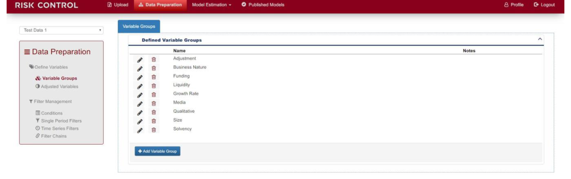
The first one, Ident, contains only information about the application. This allows Rating Engine to identify the uploaded workbook as Rating Engine data. The second sheet, VARIABLE_GROUP, lists the group names used for the analysis. We have defined the following in our demonstration: Adjustment, Business Nature, Funding, Liquidity, Growth Rate, Media, Size and Solvency, which are all assigned to continuous predictors, and Qualitative, which is assigned to all categorical variables. In fact, the names are not important. They are there to help users to group the variables in a sensible way at the modelling process. For example, one can simply define the name Raw Variables to all the continuous variables.
The third sheet has three columns: Adjusted Variable Name, Group and Definition. For each row we name the variable in the first column, the group it belongs to (no categorical variables should be listed here) and a unique ID of that variable. This unique ID under the column Definition should not contain any space characters and it is intended to be used in the application as references for combining variables to create new features.
The sheet VARIABLE_ADJUSTED_DISPLAY lists the continuous variable name (the first column value of VARIABLE_ADJUSTED_DEFINITON), the dataset name and a name to be displayed in the application.
VARIABLE_CATEGORY_DEFINITION is similar to VARIABLE_ADJUSTED_DEFINITION, but only lists information about categorical variables.
The last sheet contains the values of each categorical variables. For those variables discretized into bins, the boundaries of the bins must be specified. Note that the boundary value cannot be overlapped.
The parameter Excel workbook has a sheet “PARAMETER_SCALAR”, containing simulation, modelling and reporting parameters split into separate categories.
Uploading the variable input workbook can be done in the tab “Upload”, which should be the default first tab to be shown when the application starts.
3.2 Data Preparation
Once the variable input workbook has been successfully uploaded, one can click the tab “Data Preparation”, which collects two groups of functions to define more variable groups and combined variables, and to define filters. This can be seen in the left panel, where two groups “Define Variables” and “Filter Management” are presented. These two names can be clicked to collapse or expand their contents.
3.2.1 Define Variables
When the user clicks “Variable Groups” under “Define Variables”, the application displays the currently defined variable groups, i.e., those defined in the sheet VARIABLE_GROUP of the variable input workbook (see Figure 1).
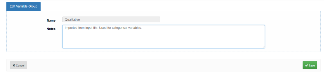
These variable groups defined in the workbook can also be edited here, for example, adding some note, by clicking the pencil icon as shown in Figure 2.
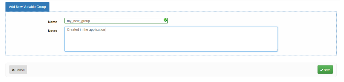
Besides defining variable groups in the input file, the user can also create new variable groups by clicking the button “Add Variable Group” in the application. This will bring up a new panel (Figure 3) in which one can provide the new group with a name and description. The name field is mandatory. A valid variable group name can be any Unicode character, such as numbers, “+”, underscores, Chinese characters, etc. But one cannot use a name that already exists.
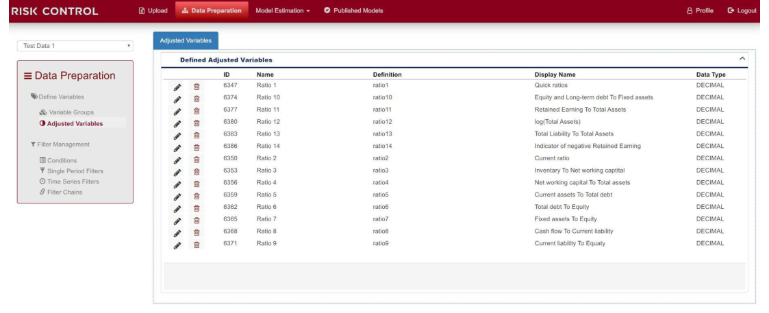
In the menu “Adjusted Variables”, the panel shows a list of variables that can be used as predictors (features) in building our model (see Figure 4). The “Name” column contains the names in the column ADJUSTED VARIABLE NAME in the uploaded input file. For variables in the Raw Variables group, the “Definition” column in this panel contains what is written in the Definition column of the input file. For categorical variables, a string of “Categorisation of” will be automatically added as a prefix.
Rating Engine can use the definition names to create new variables by combining existing ones with simple expressions. One can click the variable, or the pencil icon to edit it.
3.2.2 Filter Management
The Filter Management section groups functions to create filters. It is not uncommon during data analyses that one wishes to exclude certain records, such as those having unreasonable values for some variables, or those containing extreme numbers. Alternatively, one might wish to perform multiple analyses in each of which only a subset of the dataset is employed.
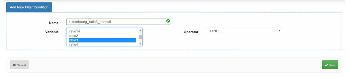
Once one is satisfied with the available variables, the next step is to click “Conditions” to define filters to exclude some data. For example, if one wishes to retain only loans for which ratio3 (Inventory to net working capital) is non-null, one may define a filter that serves to exclude observations with ratio3 variables equal to NULL. Note that the filters work by omitting data.
Figure 6: List of Defined Filter Conditions
Clicking “Add Filter Condition” will lead us to a new interface shown in Figure 5 through which one may define the filter name, the variable to which the filter is applied and the corresponding operator. Once all are specified, click “Save” and we will be back to the list of defined filters (Figure 6).
Note that the filters here defined are not yet applied to the data. They are merely definitions. Here the filters defined are simple. In other words, one may only express a variable to be null, non-null, greater, less, greater or equal, less or equal, not equal, or between or in certain value(s).
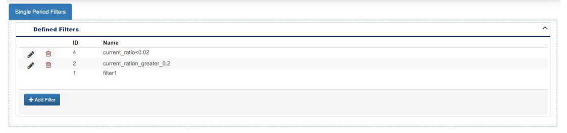
One may wonder how we specify more complex conditions, for example, requiring that ratio1 be non-null and that ratio2 is non-null at the same time? This is achieved in “Single Period Filters” (see Figure 7).
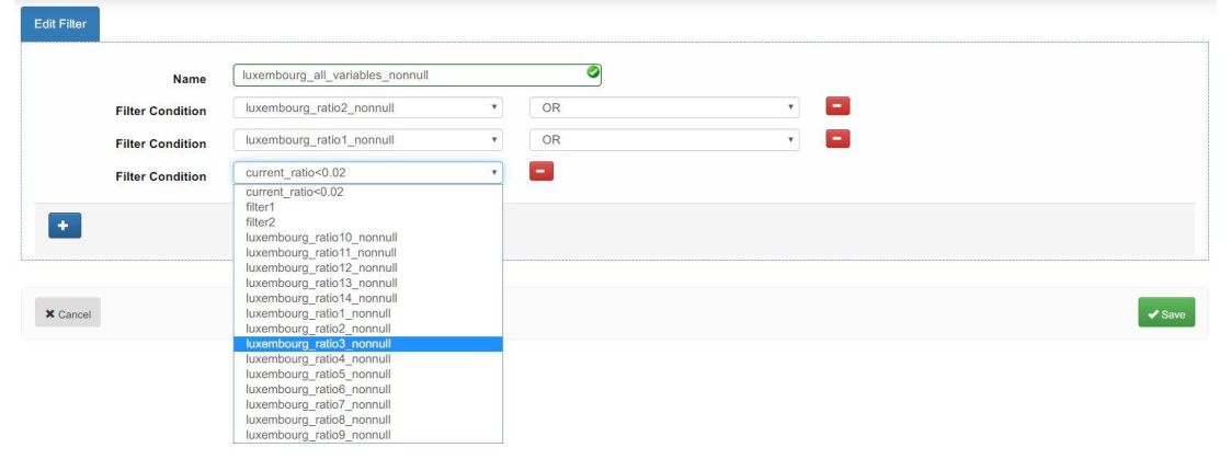
Here we will define more complex logic by combining those simple filters in Conditions. The logic operators AND, OR, NOR, XOR and AND NOT are available to us. In this demonstration, we will define a single period filter that is asking all the variables to be non-null as shown in Figure 8.
After naming the single period filter, one can build a more complex logical expression by pressing “+”, which will add a drop-down list containing the filters defined in Conditions, together with a drop-down list of logical operators. Note that although we want to apply all the simple non-null filters, we use the operator OR. This is due to the fact that filers perform actions of exclusion. One can understand it in the following way.
Suppose p represents ratio1 == NULL, and q represents ratio2 == NULL. The data we want to keep are those with ratio1 being non-null and ratio2 being non-null. To express it mathematically, one wishes to keep ¬p⋀¬q, where ¬ is logical NOT, and ⋀ is logical AND. Since a single-period filter also performs an excluding action, what we want to keep must start with ¬. Then according to de Morgan’s law, we have
¬p⋀¬q⟺¬(p∨q)
where ⋁ is logical OR. This means if we want to keep the data with ratio1 being non-null and ratio2 being nonnull, the single period filter should be defined as ratio1 being null or ratio2 being null.
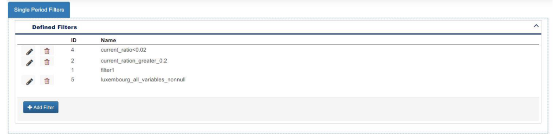
Once the filter is saved, one returns to the list of single period filters (Figure 9).
The next available option is to define time series filters. These filters allow the users to apply constraints on data from different years. Since we do not use it in this demonstration, this part will be skipped.
Finally, the last step of data preparation is to click “Filter Chains”. This part is used for combining multiple single period filters and time series filters. A filter chain is the ultimate filter that will be applied to the data for screening.
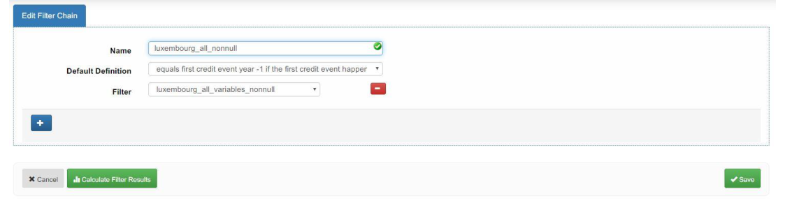
To define a filter chain (see Figure 10), one must name it and choose a definition for loan default. Then, a single period filter or time series filter can be chosen from the Filter drop-down list. If one wishes, more filters can be added and combined by clicking the “+” button.
To apply the filter chain, simply click the button “Calculate Filter Results”. Depending on the size of the dataset, this may take some time. After the calculation, three new tabs “Filter Chain Results”, “Filter Chain Cohort Results” and “Filter Chain Cohort Selection” appear in the same panel, and the bottom right button becomes “Finalise” from “Save” (Figure 11).
Figure 11: After Calculating Filter Results
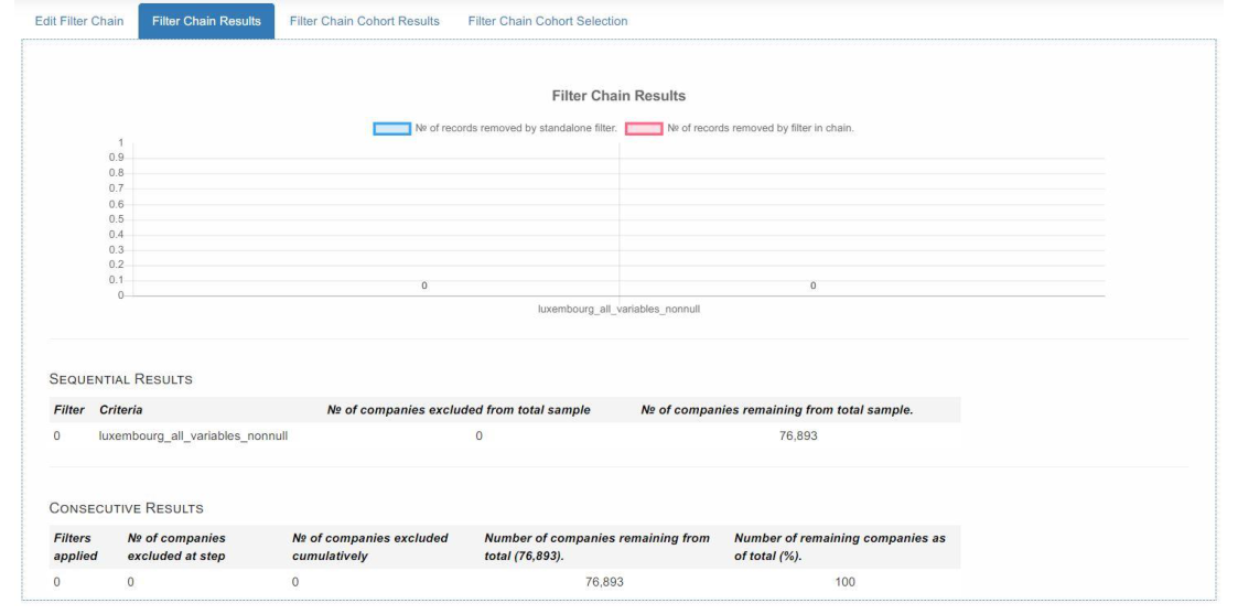
To go to the description of the data after applying the filter chain, one may click the tab “Filter Chain Results” (Figure 12). This displays the number of loans excluded by the filters one has just applied. From the image below, we may observe that, for our demonstrative example, no records were removed and all fields have nonnull values.
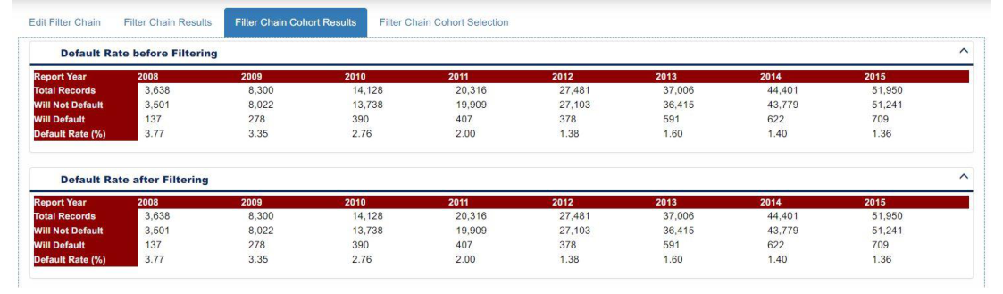
The “Filter Chain Cohort Results” tab (Figure 13) contains some statistics calculated by cohort. For example, the default rate before and after applying the filter chain.
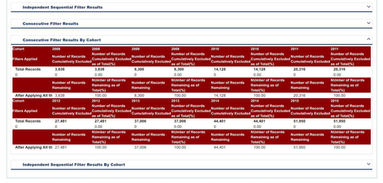
Our example shows a trend of decreasing default rate from 2008 to 2015, with the largest 3.77% in 2008. This tab also shows results of the number of records remained and removed by cohort. One can expand and collapse the results by clicking the titles (Figure 14).
The last tab “Filter Chain Cohort Selection” (Figure 15) gives the user the choice to select or deselect some cohort data based upon the results shown previously.
For this demonstration, we simply keep all the cohort years.
If one is not satisfied with the result, they can go back to edit the filter chain by clicking “Edit Filter Chain”. Otherwise, simply click “Finalise” in the bottom right corner. It will bring back the list of filter chains (Figure 16).
have already been published.
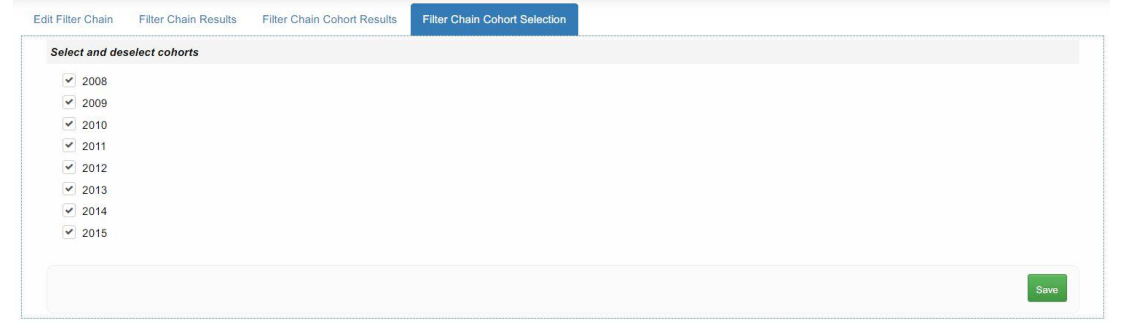
Note that once the selected cohort years are used in the modelling process, they cannot be changed anymore.
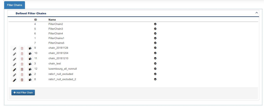
Note that in this list, those filter chains without icons at the front are those already employed in models that
3.3 Model Estimation
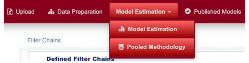
Having selected data as described above, one may turn to preparation of the model itself. Click “Model Estimation” at the top, and choose “Model Estimation” from the drop-down list (Figure 17). The other choice “Pooled Methodology” does not distinguish between different cohort years.
The user is then asked to create a model by providing a name, the used data set name and the applied filter chain. After that, click “Create Model” (Figure 18).
Figure 18: Model Creation
3.3.1 Model Creation
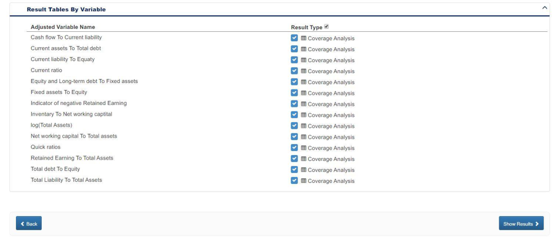
The first stage after a new model is created is “Model Creation.” At this point, the user selects all the variables that are likely to be included in the model (Figure 19). The variables can also be viewed by their groups. To select a variable, tick the box next the variable in the “Select” column. The tick boxes of the “View” column indicate whether we want coverage ratios to be calculated for the variables. Note that once a variable is decided to be left out at this stage, it can no longer be added to this model later on.
As a demonstration, we will simply select all the variables.
input workbook. Clicking “Finalise Selection” will ask Rating Engine to do coverage analyses if any box in the “View” column is ticked (Figure 20).
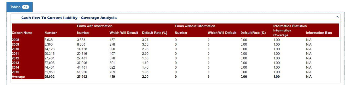
Once the calculation is complete, the user may click “Show Results”. The following image shows one example of the coverage analysis for the variable Cash flow To Current Liability (Figure 21).
These tabular results can also be exported as an Excel file by clicking “Export Tables” at the bottom. Once we are happy with the results, click “Finalise Selection”, and Rating Engine will enter into the next stage (Figure 22).
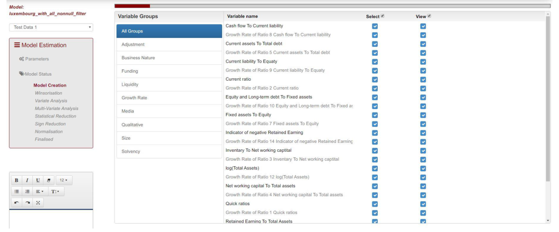
Note that the variable names when building the model are all shown with their display names we defined in the

3.3.2 Winsorisation
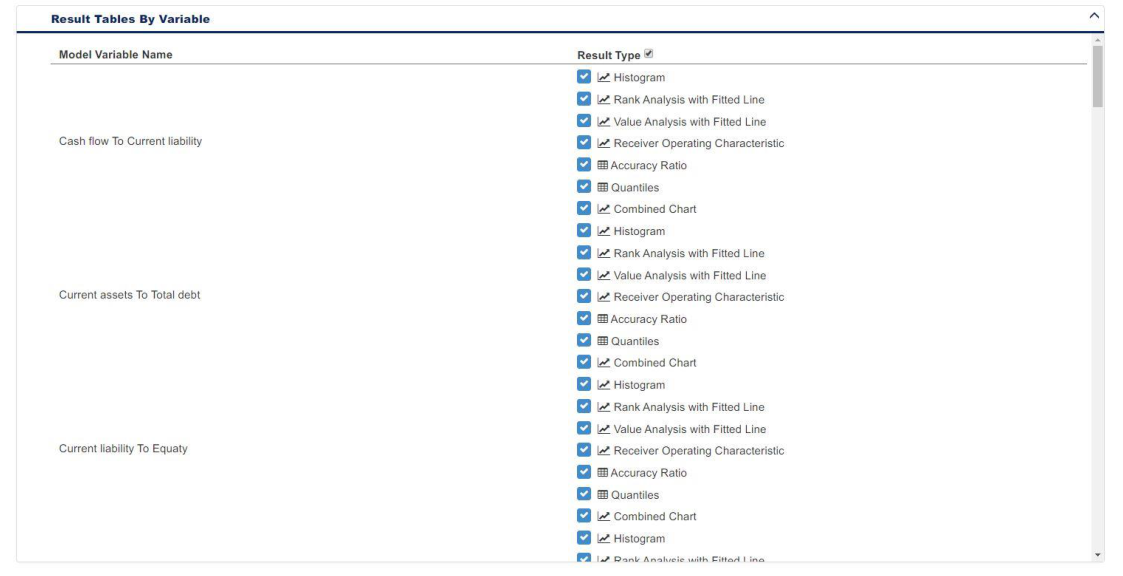
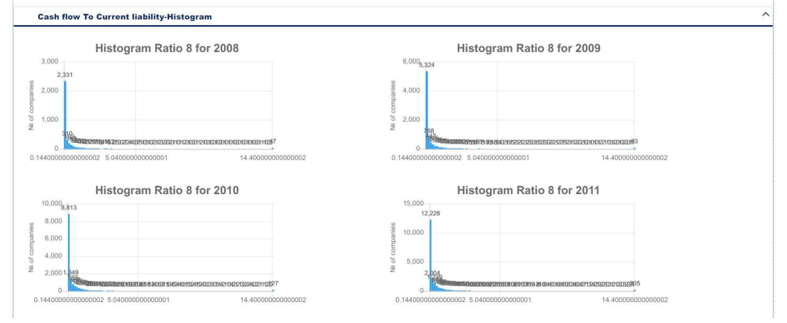
Once at the “Winsorisation” stage, we are shown a list of statistical analyses, such as histogram, rank/value regression, accuracy ratio, etc, for each variable (Figure 23). Each analysis has a tick box before it, which one can select or deselect whether or not to perform it. By default, all of them are selected.
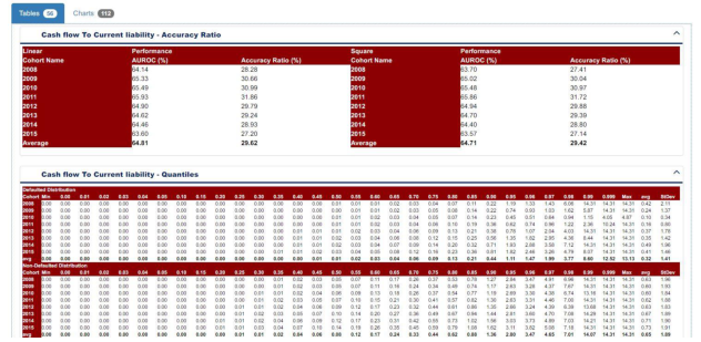
One can click “Show Results” to see histograms, rank analyses with fitted lines, quantiles, etc. These results are grouped into two tabs “Tables” and “Charts”. Figure 24 shows an example of accuracy ratio and quantiles in “Tables”.
The accuracy ratio table shows the accuracy ratios when the variable is used alone in the model as a linear term and combined with a squared term, respectively. The AUROC means the “area under the ROC curve”. The ROC curve of a binary classifier plots false positive rate versus true positive rate. The larger the area under the ROC curve, the better the performance of the classifier is. Thus, for a perfect model, AUROC is 1 or 100%. If the area is 50%, then it means the classifier is no better than random guessing. The accuracy ratio is calculated by 2 × AUROC −1. Figure 25 shows an example of histograms by cohort years produced by Rating Engine.
3.3.3 Variate Analysis
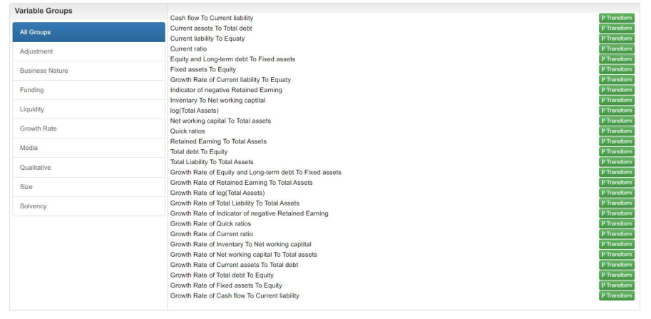
Next, click “Variables Transformation”. This leads the user to a page in which different transformations may be applied to the existing variables (Figure 26). The stage of “Variate Analysis” allows the users to perform the same statistical analyses (histogram, rank/value regression, accuracy ratio, etc.) on the transformed variables.
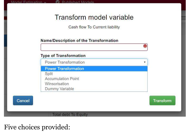
If one wishes to perform transformations, this may be achieved by clicking the “Transform” button next to the target variable. A model pop-up dialog box will show, allowing the user to choose a particular transformation (Figure 27).
• Power Transformation: for the selected variable, a logistic regression is run on all possible combinations of 2 power transformations, and based upon the AIC criterion, the best power combination will be proposed.
• Split: By providing a parameter v[0], two extra variables will be created, which are XN= min (X, v[0]) and XP= max (X, v[0]).
• Accumulation Point: By providing a parameter v[0], a dummy variable XVv[0] = 1{v[0]}(X) is created, where 1A(X) is the indicator function equal to 1 if and only if X∈A otherwise 0.
• Winsorisation: Winsorisation is also called thresholding, where an upper and a lower limit is specified and any values beyond these limits are replaced by the limiting values.
• Dummy Variable: By providing a range (v[1], v[2]], a dummy variable is created as XV= 1(v[1],v[2]](X).
For our example, we are not going to apply any transformations. In this case, one may simply click “Transform Variables” at the very bottom which will bring up a page listing all the analyses that can be performed on each variable, including the transformed ones. However, since one did not apply a transformation, this page is just like the one we were on at the stage of “Winsorisation”. Clicking “Show Results” asks Rating Engine to perform the required analyses indicated by the ticked boxes, and shows them in the tabs “Tables” and “Charts”. To proceed to the next stage, one may click “Select Variables”.
In summary, the stages “Winsorisation” and “Variate Analysis” are quite similar in that they both allow us to examine how well each variable is able to explain the data. The only difference is that we can add transformed variables at the stage of “Variate Analysis”.
One may wonder why such stages are needed as the ultimate goal is to build a multivariate model. The reason is, it is unwise to include all possible variables in the model. One must decide which predictors are likely best to explain responses. Hosmer and Lemeshow (2000) suggest to model each potential variable to determine which predictors are not contributing to the model. The two-stage approach permits one to examine variables in order to decide whether or not to include them at the next stage.
3.3.4 Multi-Variate Analysis
Users can now select different variables to build a multivariate logistic regression model. The idea is to find a linear combination of explanatory variables consisting of transformed and untransformed data, and to apply the sigmoid function to provide the best fit to the default events in the dataset. The sigmoid function commonly employed is:
σ(x) = 1 + e−βTx
Here, x is a column vector of features of the model, β is a column vector of coefficients that needs to be found. However, note that Rating Engine uses the following equation:
σ(x) = 1 + eβTx
The difference is in the signs of the coefficients.
There are different algorithms to find the “best” coefficient vector β. The one used in Rating Engine is the Maximum Likelihood method.
If a variable has been subjected to a power transformation, Rating Engine selects the best power based on the minimum AIC (Akaike Information Criterion) value. AIC is calculated as
AIC = 2k−2 ln(L̂),
Here, k is the number of estimated parameters in the model, and L̂ the Maximum Likelihood value of the model. Minimising AIC is equivalent to minimising the Kullback-Leibler divergence between the estimated model and the true unknown model.
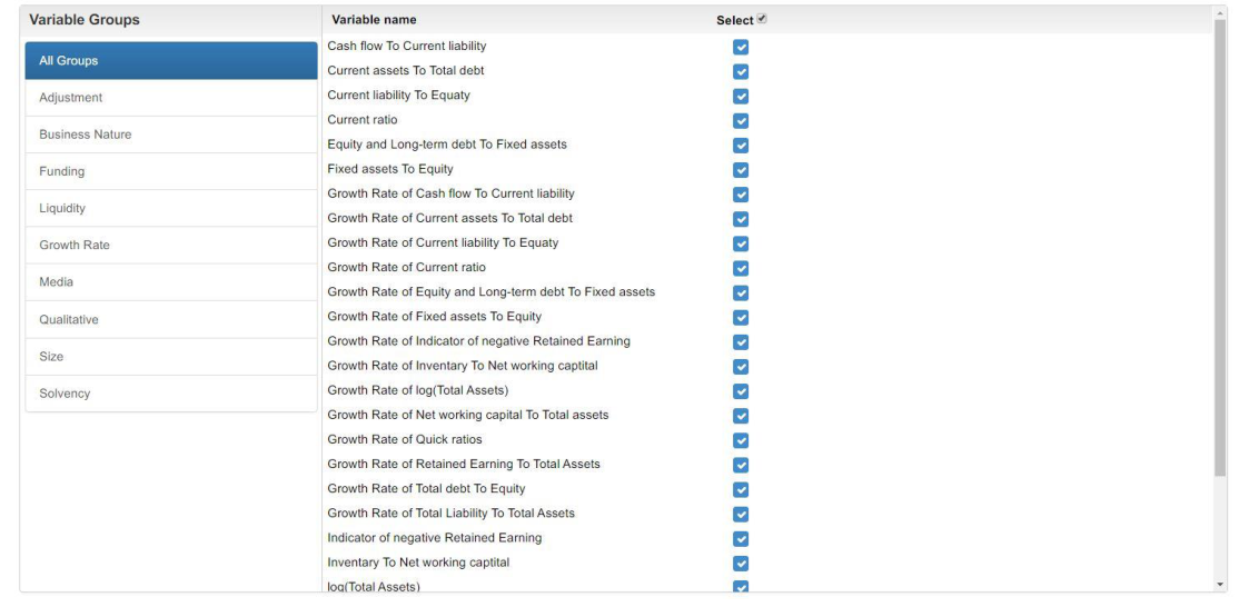
Having arrived at this stage, users are presented with a list of available variables and tick boxes to choose which are to be included as features in the multivariate model, after examining how each variable performs in a univariate model (Figure 28).
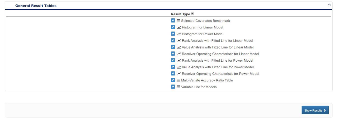
After selection, one may click “Finalise Selection”. Rating Engine will then perform analyses and select the best power transformations of variables and combinations. Once the analyses are finished, the user is prompted to choose which results he or she wishes to examine (Figure 29).
By default, every result type is selected. Rating Engine will create tables and charts after one clicks the button: “Show Results”.
3.3.5 Statistical Reduction
At this stage, Rating Engine calculates the t-statistics for the explanatory variables. Users may decide to remove certain variables based on their own judgements to reduce the number of variables. In fact, the software is testing the null hypothesis that a coefficient is 0, which means exclusion of the variable. The t-statistics tells us whether we can confidently reject the null hypothesis. Generally, high absolute values mean the corresponding variables are contributing to the model significantly.
3.3.6 Sign Reduction
Rating Engine checks whether the signs of the coefficients match those from the univariate analyses. Similar to “Statistical Reduction”, one can make a decision whether to remove those with opposite signs.
3.3.7 Normalisation
At this second to last stage, Rating Engine integrates the coefficients in different time periods. Three tasks are performed:
• For each time period, a normalisation process is realized to make sure the obtained z-score is standardized;
• The normalised coefficients are averaged over different time periods;
• The constant term is adjusted by using the real-life probability.
3.3.8 Finalised
The last stage is only a summary of the final model and the parameters in use. Once the model is finalised, it can be published by clicking the arrow before “Model ID”.
3.4 Published Models
Once the model has been published, all the information will be available for downstream systems to access default probability estimates by submitting data for one or more individual loans via web services. By clicking the “Published Models” tab, users can enter the page where all published models are shown. The “eye” button at the beginning of each model allows one to review all the tables and charts during the model building process. The “File” button at the end of each row is used to export all tables and charts generated.
4. Conclusion
This document provides a very detailed exposition of how an analyst can progress through the process of building a scoring model for loans to companies. Similar approaches may be applied to generate scoring models for other loan types like residential mortgages or consumer loans.
The novelty of the approach is that the framework offers a highly structured environment in which, subject to an agreed overall methodology, analysts perform a sequence of steps, exercising judgments at different stages, and end up with a scoring model. This process is, in fact, similar to what is commonly done in large banks that maintain loan scoring models for regulatory and business purposes.
In that context, senior managers typically determine a loan scoring methodology which may, depending on the model, also be submitted for inspection and approval by regulators and/or internal audit. The task of calibrating such models for subsets of the loan population and for updating the models over time is then delegated to less senior risk specialists. The approach implemented here facilitates such hierarchical processes of model methodology determination and delegated statistical implementation.
References
Hosmer, D.W. and S. Lemeshow (2000) Applied Logistic Regression, 2nd Edition. USA, John Wiley & Sons, Inc.
Risk Control Limited 13-14 Dean Street London W1D 3RS +44 (0)203 307 0730 www.riskcontrollimited.com
Notes
[1] The data are publicly available in the form of XBRL and iXBRL files.