

Research Paper
Estimates of Credit Spread Correlations
Date: 2002
Reference number: 2/3
Estimation of Credit Spread Correlations
Authors: William Perraudin, Marco Polenghi and Alex Taylor
Abstract The recent interest in portfolio credit risk modelling has concentrated attention on the
correlation structure of credit risk. This paper calculates long-holding period correlations for emerging market sovereign spreads and compares these with the correlations of equity market indices for the same countries.
1. Introduction
The academic literature on credit spreads has increased substantially in recent years but the focus has been on a few quite specific topics. Pitts and Selby (1983), Sarig and Warga (1989), Litterman and Iben (1991), Helwege and Turner (1999) have examined the shape of credit risk term structures (see also Kiesel, Perraudin and Taylor (1999)). Longstaff and Schwartz (1995), Morris, Neal and Rolph (1999), Duffee (1999) and Kiesel, Perraudin and Taylor (2000) study the correlation between changes in interest rates and in credit spreads. Ang and Patel (1975), Altman (1989), Kao and Wu (1990), Hand, Holthausen and Leftwich (1992), and Taylor and Perraudin (2000) investigate the relation between credit spreads and ratings.
Increased interest in the modelling returns on credit risk portfolios means the study of the correlation structure of credit risk is an important area of current research. In this field, very few studies have so far been attempted. In an important recent contribution, Varotto (2000) examines credit-related correlations in a large dataset of time series for individual Eurobonds. The interest of his study is augmented by the quality of the data employed which consists of daily observations of bond prices for several thousand straight coupon bonds, entirely free of the optionality that bedevils most empirical work on bond spreads.
Using cross-sectional regression techniques applied by Heston and Rouwenhorst (1994) to equity returns for different countries and industries, Varotto shows that there is more scope for reducing portfolio risk through cross-country diversification than through diversifying across industries. The average pair-wise correlation for bonds in Varotto’s sample is 19%. Within countries, the average correlations are 15% for bonds issued by US-domiciled obligors and 16% and 23% for bonds issued by obligors from Japan and the UK respectively.
This paper contributes to knowledge regarding credit risk correlations by studying a particular part of the credit markets, namely dollar-denominated sovereign Eurobond markets. There are three stages in the analysis. First, daily time series of spreads are extracted from bond prices. Second, correlations in long horizon changes in spreads and log equity prices are calculated, using overlapping daily data as suggested by Kiesel, Perraudin and Taylor (1999). Third, quadratic programming techniques are employed to merge the equity- and spread-based correlation matrices so as to obtain a single matrix that can be used in credit risk modelling.
2. Data
The data used in the study consisted of: A. Daily bond mid-prices for 20 countries: Argentina, Brazil, China, Colombia, Hungary, Iceland, Indonesia, Mexico, Russia, Slovenia, Thailand, Costa Rica, Croatia, Greece, Lithuania, Philippines, South Korea, Tunisia, Venezuela and Portugal. B. Time series yield data for US government pure discount bonds. These are necessary in order to infer spreads on the defaultable sovereign bonds. C. Equity index data for a large group of stock market indices (including both country and industry indices). The source of the bond price data is Bloomberg™. The bonds are selected according to the following criteria:
1. The currency is US dollar denominated.
2. The coupon is fixed.
3. The bond has not expired.
4. The bond is neither call nor put features has no sinking fund. Applying these stringent criteria, one obtains a dataset containing 49 individual bonds. When there are multiple bonds for a given sovereign, the bond with the largest number of daily price observations is selected.
The US strip yield data goes from 16th April, 1991 to the present and includes 3 months, six months, 1-5,7,10, 20 and 30 years maturities. Data for the additional maturities 8, 9,15 and 25 years starts on 10 April 1996. In calculating spreads, one needs yields for specific maturities including fractions of years. To obtain these, we interpolate the adjacent yields for annual maturities in a straightforward fashion.
The bonds in our data set are listed in Table 1. As is apparent, the sample periods in which individual bond prices are observed vary considerably. Some bonds are only observed for the last two years while others are observed for more than seven years. While this is not apparent from the table, the data suffers from the additional problem that for periods within the sample ranges, there are missing observations.
3.Techniques
The first task to be tackled is that of extracting a daily time series of spreads against US Treasury yields for each bond. In principle, one might expect that both spreads and default free yields would have their own term structure in that spreads and yields at long maturities would differ from those at short maturities. This would suggest that to extract spreads, one would have to employ term structure fitting techniques such as those used on defaultable bond prices by Schwartz (1998) and Perraudin and Taylor (2000). These techniques yield flexible estimates of credit term structures but require large numbers of bonds to produce reliable estimates. Since relatively few emerging market sovereign bonds are available and because we wished to infer spreads for individual sovereigns, it was necessary to consider simpler approaches.
We therefore assume that while the default free term structure is unrestricted, the term structure of credit spreads for individual sovereign borrowers is flat. In this case, given estimates of the default free term structure, one may extract a credit spread from a single observation of a defaultable bond price. This involves, for each date t in the data set, inverting the following equation to find a time series of values St
N Pt − ∑exp[− Rt,t( j) (t( j) − t) ] exp[− St (t( j) − t) ] d j = 0 . j=1
Here, Pt is the market price of the bond at date t and Rt,j is the yield at date t on a US Treasury strip with maturity T-t and dj is the coupon payment on the bond paid at date t(j).[1]
One may ask whether the assumption of flat term structures is too strong. Simulation of structural corporate bond pricing models suggests that high quality credit spreads are upward sloping and low credit quality spreads are hump shaped (see, for example, Selby and Pitts (1983)). Actual market data for credit spreads, however, suggests that spreads are much flatter than theoretical models imply (see the Bloomberg spread means provided in Kiesel, Perraudin and Taylor (1999)). Hence, the approximation in assuming flat spreads is probably not excessively strong.
The second step in our analysis is the estimation of correlations between different spreads. We are primarily interested in long holding period correlations relevant for credit risk modelling. Kiesel, Perraudin and Taylor (1999) show that spread correlations calculated for one day holding periods may be very different from those that apply over long holding periods such as six months or one year. They advocate simple nonparametric techniques for estimating long horizon moments of spread changes.
In essence, the Kiesel-Perraudin-Taylor technique consists of (i) estimating longhorizon moments of changes in the series using highly overlapping observations of changes (with daily data, an overlapping observation moment estimator for say a year will involve very substantial overlap between successive observations), and (ii) calculating asymptotic corrections for biases that arise from the use of overlapping observations. The bias corrections are calculated assuming that the series is a pure random walk. For a long horizon, the random walk component of the series will dominate so adjusting as though the series were a random walk is appropriate.
The moments that interest us here are correlation coefficients, i.e., the ratio of the covariance between two series to the product of the standard deviation of each series. If the numerator and denominator in this ratio were independent of each other, then since the bias corrections for the numerator and denominator are equal, the correction would cancel. In this case, one may simply calculate an unbiased correlation estimate using the uncorrected covariance and standard deviation estimates. Of course, the numerator and denominator are not independent but the order of bias induced is less than that created by the use of overlapping observations. We, therefore, follow the simple approach of working with a ratio of uncorrected moments.
A complication that arises with our data and which is absent from the data employed by Kiesel, Perraudin and Taylor is that the data periods covered by the different series are not the same. Even within the ranges of dates for which we observe spreads for two series, one of the series may have isolated missing observations. These problems mean that the number of observations available to us is quite small if we insist on calculating spread correlations using overlapping observations of, for example, spread changes over a fixed period, such as one year.
To cope with this problem, we (i) calculate individual correlations for spreads i and j, say, using all the observations for which both i and j spreads are observed for which there exists in the data set a change over at least as long a period as the given horizon. In other words, if we are interested in spread changes over six months, we employ any t-dated pair of i and j spreads for which there is a pair of spreads observed at least six months earlier in the sample. To be slightly more formal, if our desired horizon is K, for any date t, we include in the estimator suitable scaled squared spread changes from t minus K’ to t where K’ is the smallest integer greater than K for which we observe data at t-K’. This approach implies that data period for the i and j spread pairs is then not, in general, the same as the period for which i and k spreads are observed.
Mathematically, our covariance estimator is defined as:
N S − S K 1 ⎛ ,1t(N) ,1t(1) ⎞ S,1t( j) − S,1t( j)−k( j) − ∑ ⎜ ⎟ N −1 j=a k( j) ⎝ (t(N) − t)1()/ k( j) ⎠ S − S ⎛ ,2t(N) ,2t(1) ⎞ ×⎜ S,2t( j) − S,2t( j)−k( j) − ⎟ (t(N) − t)1()/ k( j) ⎝ ⎠
Here, the sample of observations j=1,…,N, consists of N successive observations which are not necessarily observed on successive days but for each of which, both the spreads
S1,t(j) and S2,t(j) are observed. By convention t(1)=1. The constant K is the number of days for which one wants to calculate the holding period covariance. For each observation date, t(j), the quantity t*(j) is the latest date for which t*(j)<t(j)-K and the spreads S1,t*(j) and S2,t*(j) are observed if this date exists and otherwise equals 0. k(j) is defined as t(j)-t*(j) and a ≡ min{2,1,..., N such that t *(i) > 0} . Finally, in order to obtain the correlation, we compute the two variances over the same period used to compute the covariance.
The equity correlations are also estimated using the overlapping observation approach described above except with a common sample period and with changes in the log equity indices always over the same period. (Their estimation is not therefore subject to the complications described above that affect the spread correlations.)
The ready availability of equity index data means that it is much easier to obtain country and industry factor correlations based on equity correlations than it is to derive spread-based correlations in the way described above. A reasonable approach is then to combine spread-based correlation matrix in some way with the equity-based correlation so as to create a more accurate estimate of the correlation structure of the complete set of factors.
The third task we, therefore, need to address is that of incorporating the spread correlation estimates into a larger matrix of equity correlations. It is not possible simply to replace sub-matrices within an estimated correlation matrix with a correlation matrix estimate generated using some other technique. The reason is that the resulting matrix will generally not be positive definite and so will not be useable in other statistical exercises required in credit risk modelling such as the generation of correlated random variables.
The approach we suggest consists of updating a matrix of equity-based correlations using the information contained in the spread correlation matrix by minimizing a quadratic distance function between a parameterised covariance matrix and the estimated equity- and spread-based matrices. The parameterised covariance function is assumed to have a factor structure since this provides a simple way of limiting the number of parameters to be fitted while maintaining positive definiteness.
To be precise, let E denote a 176x176 matrix of correlation coefficients for a large set of country and industry equity indices.[2] Let S denote an 18x18 correlation matrix estimated from spreads. Let E* denote the parameterised 176x176 estimator of E. Let
* ES denote the 18x18 sub-matrix of E* with rows and columns correspond to the countries in S.
Because all the matrices we encounter are symmetric and have unit diagonal elements, we can restrict our attention to elements contained in the lower diagonal part. The vech(.) operator applied to a matrix yields a the lower diagonal part of the matrix (i.e., the elements below the leading diagonal) in a vectorized form in which columns are stacked one above the other starting from the left-most column.
One may obtain an estimate E* of E by minimizing the following function over the elements of the vectors b[1], b[2], .. , bN.
2 * L = λ[vech(E*) − vech(E)] + (1−λ)[vech(ES ) − vech(S)]
N 2 2 2 where E* = ∑i=[1]bibi '+Q and Q is a matrix having 1− bi1, − bi,[2] − ..−bi,N in the diagonal element on the ith row, and zeros off the diagonal.
4.Results
Spread Estimates Spreads for the different sovereigns are extracted from bond prices for all the available days in the data set. The periods in which bond prices are available are listed in Table 1. Few of the bond price series have prices observed on every day in the periods specified in Table 1. The numbers of daily (working day) observations available for each bond is shown in Table 2. Countries with large numbers of observations include Argentina, Brazil, China, Indonesia, Russia and Portugal. Countries such as Costa Rica with relatively few observations are likely to produce less reliable correlation estimates.
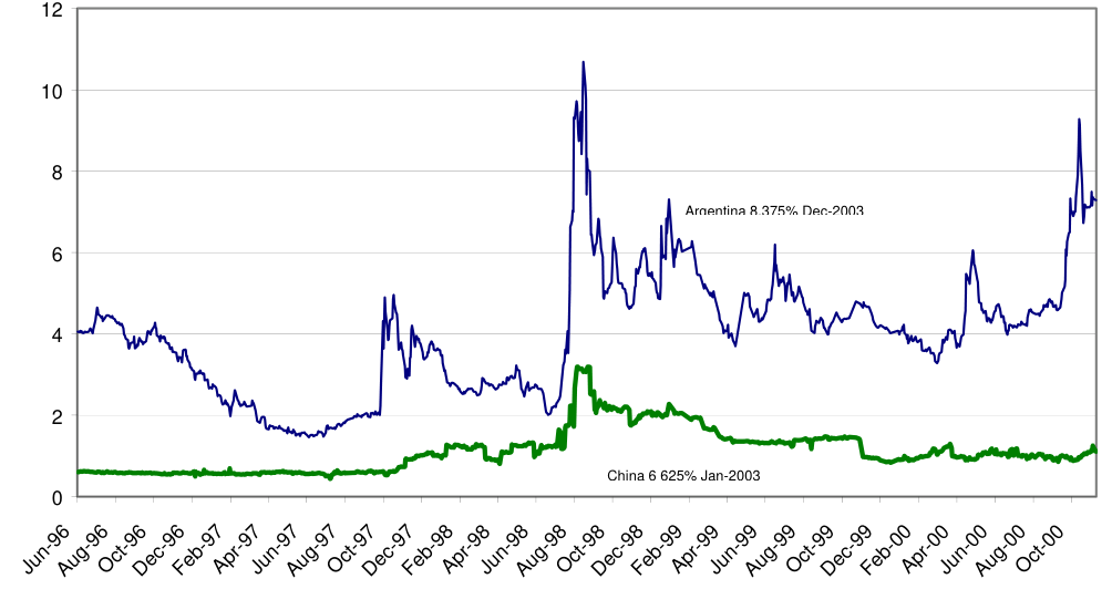
Examples of the spread time series are shown for Russia in Figure 1, and for China and Argentina in Figure 2. The Russian and Asian crises are clearly identifiable from the correlated jumps in the estimated spreads.
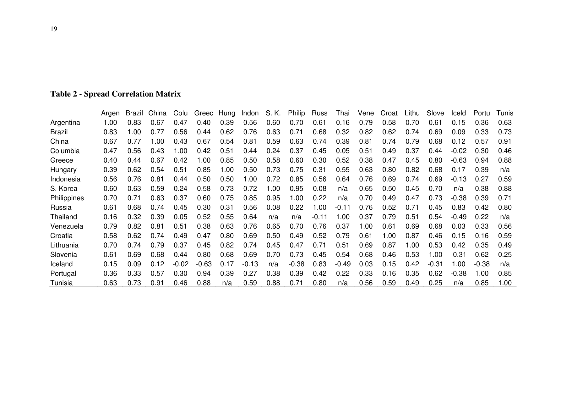
Correlation Estimates Estimates of one-year spread correlations are shown in Table 3. The correlations are virtually all positive and the over all average spread correlation between the emerging market countries (i.e., the average of available entries off the diagonal in the correlation matrix) is 0.45. Some correlations for pairs of countries that have limited overlapping estimated spread data are shown in Table 2 as not available. No correlations were estimated for Mexico or Costa Rica because the numbers of overlapping observations with most other countries were too few.
The estimates seem quite sensible in most cases. For example, Argentina spreads are closely correlated with Brazil for example, and more weakly correlated with European countries such as Hungary, Iceland etc. Some correlations like the relatively high correlation between Lithuania and Argentina seem less reasonable.
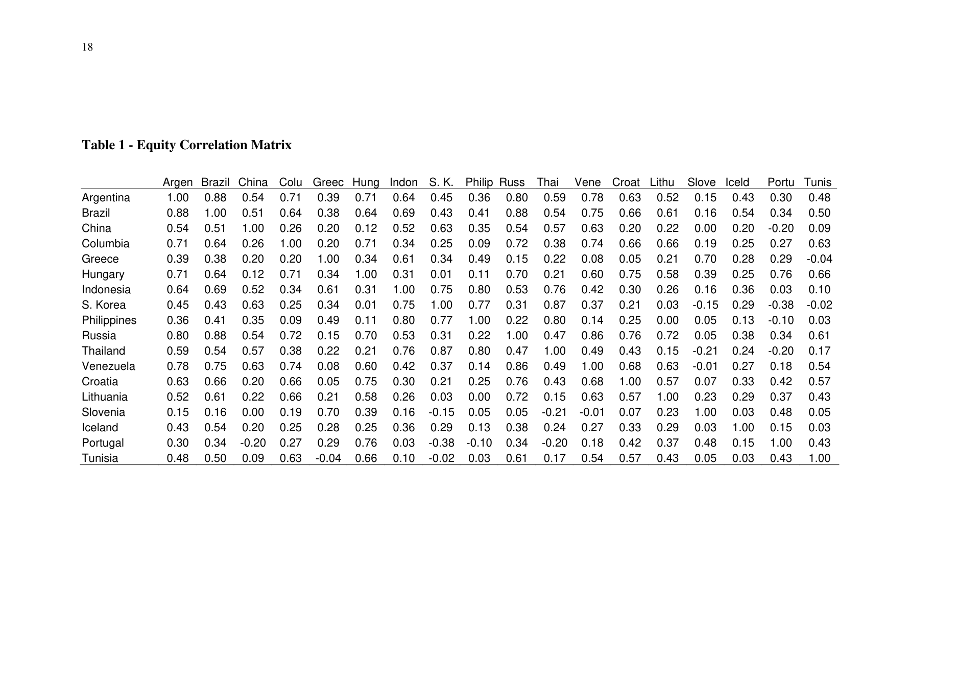
Equity correlations for the countries for which we estimate spread correlations are shown in Table 4. It is interesting that some features of the spread correlations that appear surprising reappear in the equity correlations. For example, equity returns for China and Argentina are relatively closely just as are Chinese and Argentine spreads. The same is true for Russian and Argentine equity returns and spreads.
Over all comparisons between the equity and the spread correlations are shown in Table 5. For the 18 countries for which we have both spread and equity correlations the average equity spread correlations is 49.56%, which is slightly lower but reasonably close to the average of the available spread correlations, i.e., 45.27%.
Merging Spread- and Equity-Based Correlation Estimates The estimated spread correlation matrix reported in Table 3 is not positive definite. This is not surprising because the elements of the correlation matrix are calculated using different sample periods. But the observation motivates the fitting of the correlation matrix to a parameterised matrix that is positive definite so it can be used in credit risk modelling to generate correlated random numbers.
The most convenient positive definite correlation matrix parameterisation is that described in the last section in which it is assumed that the correlation matrix is that of a vector of random variables satisfying a factor structure. In this case, the nxn dimensional correlation
N matrix may be written as ∑i=[1]bibi '+Q where the bi are n-dimensional vectors and Q is a
2 2 2 matrix having 1− bi1, − bi,[2] − ..−bi,N in the diagonal element on the ith row, and zeros off
the diagonal.
We minimize the distance function given in the last section with respect to the bi assuming different numbers of factors (i.e., different values of N in the above notation). A larger number of factors implies a larger number of parameters to fit the correlation matrix and hence a better approximation. Having minimized the distance function, one obtains a set of
N ˆ ˆ b bˆ '+Q fitted vectors bˆi and a fitted correlation matrix ∑i=[1] i i .
One way to measure the accuracy of fitted correlation matrices is to see how rapidly they stabilize as one increases the number of bi’s, i.e., N. Figure 3 shows the ratio of the ordered eigenvalues of matrices fitted with 1, 2, and 3 factors to the ordered eigenvalues of a matrix fitted with 4 factors. It is noticeable that the ratios settle down rapidly to values just above unity for the 3-factor case. This suggests that the approximation is reasonably close.
Another way to show how close the fitted matrix is to the approximating matrix is to examine the average discrepancy between the individual correlations in the original equity factor correlation matrix for 176 factors and the corresponding individual correlations in the fitted matrix. Figures 4-7 show histograms of the differences between the equity and the fitted correlations.
Lastly, one may examine the comparisons in average correlations contained in Table 3. The average correlation for all 67 equity index factors for countries in our dataset is 32.56% and this is exactly equal to the average of the fitted matrix for country correlations based on four factors. The average correlation for the large matrix of 176 country and industry equity factors and commodity prices is 28.59%. The average correlation for the fitted matrix with equity and spread correlations merged assuming four factors is 28.65. These results suggest (i) that four factors fit the correlation structure reasonably well, (ii) that the spread correlations are on average slightly lower than the equity indices for the same countries although not wholly out of line.
Russia 3% May 2003 Spreads in percent 30
Jun-96Aug-96Oct-96Dec-96Feb-97Apr-97Jun-97Aug-97Oct-97Dec-97Feb-98Apr-98Jun-98Aug-98Oct-98Dec-98Feb-99Apr-99Jun-99Aug-99Oct-99Dec-99Feb-00Apr-00Jun-00Aug-00Oct-00 Dates
Figure 2 - Spreads for Argentine and Chinese Government Bonds
3.5
2.5 λ1/λ4 2 λ2/λ3 Ratio 1.5 λ3/λ4
0.5
15 29 43 57 71 85 99 113 127 141 155 169 Eigenvalue number
Figure 3 - Eigenvalue ratios. We plot the ratios between the eigenvalues with 1, 2
Frequency
0.03 0.20 0.37 0.53 0.70 -0.81 -0.65 -0.48 -0.31 -0.14
Figure 4 - Error distributions of the difference between the original factor correlation matrix and the one estimated with 1 factor
Frequency
0.10 0.23 0.37 0.50 -0.72 -0.58 -0.45 -0.31 -0.18 -0.04
Figure 5 - Error distributions of the difference between the original factor correlation matrix and the one estimated with 2 factors
Frequency 10
0.11 0.25 0.39 0.53 -0.71 -0.58 -0.44 -0.30 -0.16 -0.02
Figure 6 - Error distributions of the difference between the orginal factor correlation matrix and the one estimated with 3 factors
Frequency
0.04 0.14 0.25 0.35 0.45 -0.48 -0.38 -0.28 -0.17 -0.07
Figure 7 - Error distributions of the difference between the original factor correlation matrix and the one estimated with 4 factors
Country Coupon Rate (%) Maturity Date First Obs Last Obs. Argentina 8.375 20-Dec-03 23-Sep-94 5-Dec-00 Brazil 8.875 05-Nov-01 22-Nov-96 5-Dec-00 China 6.625 15-Jan-03 23-Jan-96 5-Dec-00 Columbia 7.250 15-Feb-03 14-Feb-96 5-Dec-00 Hungary 8.800 01-Oct-02 1-Feb-93 16-Dec-99 Iceland 6.125 01-Feb-04 3-Feb-94 5-Dec-00 Indonesia 7.750 01-Aug-06 26-Jul-96 6-Nov-00 Mexico 8.500 15-Sep-02 11-Jan-93 5-Dec-00 Russia 3.000 14-May-03 28-Jun-96 5-Dec-00 Slovenia 7.000 06-Aug-01 22-Jul-96 5-Dec-00 Thailand 8.250 15-Mar-02 25-Mar-92 28-Feb-00 Costa Rica 8.000 01-May-03 23-Apr-98 11-Oct-00 Croatia 7.000 27-Feb-02 6-Feb-97 5-Dec-00 Greece 6.950 04-Mar-08 27-Feb-98 5-Dec-00 Lithuania 7.125 22-Jul-02 8-Jul-97 5-Dec-00 Philippines 8.875 15-Apr-08 2-Apr-98 5-Dec-00 South Korea 8.875 15-Apr-08 9-Apr-98 5-Dec-00 Tunisia 7.500 19-Sep-07 26-Feb-99 5-Dec-00 Venezuela 9.250 15-Sep-27 11-Sep-97 5-Dec-00 Portugal 5.750 08-Oct-03 20-Sep-93 5-Dec-00
Country Mean(%) Std. Dev. Max Num. Of obs. Argentina 4.323 1.613 10.689 1490 Brazil 3.304 2.358 17.741 1037 China 1.077 0.554 7.316 1267 Columbia 2.843 1.618 9.781 898 Hungary 0.981 0.416 3.267 635 Iceland 0.549 0.241 2.291 965 Indonesia 4.785 3.373 17.083 1012 Mexico 2.987 2.246 14.050 708 Russia 21.425 20.430 77.401 998 Slovenia 0.686 0.234 1.858 1085 Thailand 1.387 1.133 8.313 782 Costa Rica 2.126 0.733 3.957 178 Croatia 2.979 1.470 9.229 882 Greece 0.878 0.295 7.438 721 Lithuania 2.484 1.042 7.088 710 Philippines 3.835 1.234 9.206 687 South Korea 3.563 1.520 9.859 690 Tunisia 1.706 0.431 8.225 461 Venezuela 7.416 2.377 17.089 825 Portugal 0.321 0.229 6.880 1872 matrix and for the fitted sub-matrix for the country factors
Numbers of factors Large Small 1 0.28035 0.29744 2 0.28580 0.30124 3 0.28662 0.32277 4 0.28654 0.32567
| Country All factors Country factors | factors |
|---|---|
| with | spreads |
| Average equity 0.286 0.326 | 0.496 |
| correlations | |
| Average spread | 0.453 |
| correlations |
Bibliography Altman, E., 1989, “Measuring Corporate Bond Mortality and Performance.” Journal of Finance 44, 909-922.
Ang, J. and Patel, K., 1975, “Bond Rating Methods: Comparison and Validation.”, Journal of Finance, 30, 631-40.
Duffee, G.R., 1999, “Estimating the Price of Default Risk.” Review of Financial Studies 12, 197-226.
Hand, J., Holthausen, R. and Leftwich, R., “The Effect of Bonding Rating Agency Announcements on Bond and Stock Prices.” Journal of Finance 47, 733-52.
Hand, J., Holthausen, R. and Leftwich, R., “An orderd Probit Analysis of Transaction Stock Prices.” Journal of Financial Economics 31, 319-79.
Helwege, J., and C. Tuener, 1999,” The Slope of the Credit Yield Curve for Speculative Grade Issues” Journal of Finance 50, 789-819.
Kao, C. and Wu, C., 1990, “Two Step Estimation of Linear Models with Ordinal Unorbserved Variables: the Case of Corporate Bonds.” Journal of Business and Economic Statistics 8, 317-25.
Kiesel, R., Perraudin, W. and Tayor, A.P., 1999, “The Structure of Credit Risk.”, Working paper, Birbeck College, London.
Kiesel, R., Perraudin, W. and Tayor, A.P., 2000, “Credit and Interest Rate Risk” unpublished Bank of England mimeo.
Longstaff, F.A., and Schwartz, E.S., 1995, “A Simple Approach to Valuing Risky Fixed and Floating Rate Debt.” Journal of Finance 50, 789-819.
Litterman, R., and T. Iben, 1991, “Corporate Bond Valuation and the term Structure of Credit Spreads.” Journal of Portforlio Management, v17, 52-64.
Morris, C., Neal, R. and Rolph, D., 1999, “Credit Spreads and Interest Rates.” Indiana University mimeo, March.
Pitts, C.G.C, and M.J.P.Selby, 1983, “The Pricing of Corporate Debt: a Further Note.” Journal of Finance 38, 1311-1313.
Sarig, O. and A.Warga, 1989, “Bond Price Data and Bond Market Liquidity.” Journal of Financial and Quantitative Analysis 24, 367-378.
Schwartz, T., 1998, “Estimating the Term Structure of Corporate Debt.” Review of Derivatives Research 2(2-3), 193-230.
Varotto, S. 2000, “Credit Risk Diversification and Bank Capital” Bank of England Mimeo.
Notes
[1] The inversions were performed using a standard quasi-Newton root finding algorithm written in Gauss.
[2] In fact, the 176 include a small number of commodity price indices as well.