

Key findings
- Agency ratings cannot be ignored as measures of bank credit quality but they should be combined with other data sources
- Particularly since the crisis, bank ratings have appeared to show too much inertia
- In more normal times, agency ratings may be more reliable but in post crisis situations, their dynamics are questionable
- It is concerning that the rank order of ratings has recently been so little related to those of the other indicators
- The other measures are not fully convincing alternatives as they appear too volatile (equity-based measures), limited by illiquidity, availability and risk premia (CDS-based measures) and are not plausible discriminators of risk (in the case of risk weights)
- The lesson for investment institutions using credit risk indicators is that multiple indicators should be combined and used as inputs to internal rating processes
Introduction
Bank counter-party risk became a major issue for many market participants during the recent financial crisis. The risk was complex and involved multiple dimensions. Fluctuations in risk occurred not just as the financial state of banks fluctuated but also because the capacity and willingness of sovereigns to rescue banks changed over time.
Major corporates, non-bank financial firms and public bodies such as central banks struggled to monitor and manage bank counter-party risk during the crisis. Many made changes in their bank-related risk policies including altering the ways in which they set limits for bank counter-parties.
The risk of defaults by banks has significantly abated since the crisis as is evidenced by declines in spreads on bank debt and Credit Default Swaps (CDS). The reduction in such risks reflects the tightening of bank regulation since the crisis especially in the areas of capital and liquidity rules. But bank credit risk remains important and market participants should consider whether they have in place the infrastructure and procedures necessary for measuring bank credit risk in an accurate and timely fashion.
This note provides perspectives on different measures of credit risk applicable to bank exposures. We compare several approaches to, specifically (i) agency ratings, (ii) a combination of simple financial ratios suggested by regulators, (iii) Merton-style default probability estimates based on equity to liability ratios, and (iv) spreads on CDS.
The note is organised as follows. Section 1 describes the four credit risk indicators on which we focus. Section 2 gives information on the illustrative sample of banks we study. Section 3 presents results on how the risk measures have performed since the crisis. Section 4 concludes.
1. Credit Risk Measures
In this section, we describe four credit risk indicators applicable for banks. These are: agency ratings, a simple combination of financial ratios recently suggested by the Basel Committee, equity-based measures and spreads on CDS.
1) Agency ratings
Agency ratings for banks are the most obvious basis for bank counter-party risk measurement. Several thousand banks are rated worldwide and the vast majority of banks that provide counter risk for market participants are rated by one of the three major international ratings agencies.
However, bank ratings provided by agencies have been subject to criticism by regulators and researchers in recent years. For example, a recent ECB research paper, Hau, Langfield and Marques- Ibanez (2012) argues that the rank orderings implicit in ratings differ substantially from the rank orderings of equity-based risk indicators two years later. They analyse discrepancies between the two rank orderings and suggest that ratings agencies favour (i) large banks and (ii) banks that issue many securitisations. They speculate that this reflects competitive pressures on ratings agencies to confer favourable ratings on banks that provide them with significant income flows.
Certainly, bank rating criteria have in the past been insufficiently focussed on liquidity, access to stable and diversified funding sources and exposure to complex potentially illiquid investments like securitisations. But risk scoring systems employed by regulators such as the US OCC’s CAMELS and the UK FSA’s ARROW framework were similarly defective in emphasis. There is a danger of concluding too much from datasets heavily influenced by the last decade in which our understanding of banks’ vulnerability to liquidity crises has significantly changed.
2) Regulatory risk weights
A recent Basel Committee consultative paper, BCBS (2014b), sets out proposals for Standardised Approach bank risk weights for exposures to other banks. These risk weights are obtained from a simple lookup table in which entries depend on simple financial ratios: the bank’s Common Equity Tier 1 (CET1) ratio and its Net Non-Performing Asset (NNPA) ratio.
Table 1 shows how risk weights depend on these two indicators. The more dominant determinant among the two is CET1. Overall, risk weights vary from 30% for highly capitalised banks with low nonperforming assets to 300% for banks with a low CET1 ratio.
The approach to risk weights for exposures to banks proposed by BCBS (2014b) would replace the current Basel II approach in which such risk weights depend on agency ratings (either of the bank itself or of the sovereign of the country in which the bank is domiciled).
The motive for replacing agency ratings with financial ratios as determinants of risk weights for banks is that of reducing dependence on ratings. The US authorities have already gone down this path domestically with the Dodd-Frank Act while other jurisdictions such as the European Union have it as a long term goal.
BCBS (2014b) states that the calibration exercises the Basel Committee has through in calibrating the sensitivities in Table 1 suggest that the two financial ratios involved provide better predictions of bank default than do agency ratings.
A drawback of such financial ratios is that they are not available for many banks. (The denominator of the CET1 ratio equals the volume of Basel III risk weighted assets. This quantity is only available for a few banks and, for these, only for very recent time periods, CET1 and NNPA will certainly not provide very timely indicators of credit quality because of infrequency and delays in publishing such accounting measures.
| CET1>=12 | 12%>CET | 9.5%>CET | 7%>CET1 | 5.5%>CET | ||
|---|---|---|---|---|---|---|
| % | 1>=9.5% | 1>=7% | >=5.5% | 1>=4.5% | CET1>4.5 | |
| NNPA<=1% | 30% | 40% | 60% | 80% | 100% | 300% |
| 1%<NNPA<=3% | 45% | 60% | 80% | 100% | 120% | 300% |
| 3%<NNPA | 60% | 80% | 100% | 120% | 140% | 300% |
3) Equity-based indicators
The insights of Merton (1974) suggest how one can infer probabilities of default for corporate borrowers from bank equity capitalisation and debt data. Merton’s idea was that equity and debt are both options written on the underlying asset value of the firm.
From the time series behaviour of a firm’s equity market capitalisation, one may infer the volatility of its underlying assets. To work out the probability of default, one may then calculate how many standard deviations of asset value must be lost before the firm’s assets fall below its liabilities.
Banks are highly levered firms for which ratios of debt to equity are much higher than conventional corporations. Because of this, some have questioned whether equity-based modelling is applicable for banks. Also, the possibility of bank bailouts, which will certainly affect credit risk, will not be allowed for in models of the type Merton had in mind.
Nevertheless, equity-based indicators of bank credit quality have several advantages. First, they may be implemented for a large number of banks since high frequency equity capitalisation data and low frequency total liability data are readily available.
4) CDS spreads
Credit spreads are an obvious source of information on bank credit spreads. CDS spreads offer advantages in that they are available for standardised contracts and the market in which they are traded is generally regarded as quite liquid (more so than the market for bank bonds although less so than the equity market).
One may note that, unlike the equity-based indicators just described, spreads on CDS reflect risk adjusted expected losses rather than simple probabilities of default. In other words, they are affected by the recovery rate expected by the market on the bonds that a party writing the CDS would deliver.
Second, even if one knew the recovery rate and hence could infer the default probability, this latter would be risk adjusted. This means that it will be boosted by an amount that reflects how much the default tends to occur in states of the world in which investors are experiencing low returns.
A third drawback of CDS spreads as an indicator of credit quality is that they are not available for all banks that one might wish to analyse.
2. Data for a Sample of Banks
We will illustrate the risk indicators we consider using data on banks since the crisis. Our comparisons should be seen as illustrative rather than comprehensive but we believe they help to shed light on the issues involved.
We began by collecting data on 87 banks for which total assets exceeded €5 billion and the following information was available on Bloomberg: (i) S&P long time issuer rating, (ii) Tier 1 common equity ratio (CET 1 ratio), (iii) total loans, (iv) non-performing assets, (v) provisions for loan losses (the last three are used for approximating Net NPA ratio) and (vi) risk weighted assets.
Note that to approximate the NNPA ratio we used total loan, non-performing asset, provisions for loan losses from Bloomberg via the following formula:
non perfroming asset−provisions for loan losses Net NPA Ratio= (1) total loan
After deleting banks for which daily market capitalisation data is not reported for more than 100 working days during 01/01/2007-09/04/2015, we are left with 55 banks. Of these, 22 banks have CDS spread data available on Reuters (on 31/12/2014) so we restricted attention to these banks.
The methodology employed in calculating the equity-based default probabilities is described in the Appendix.
On CDS spreads, we adjust the spreads to obtain implied default probabilities. We achieve this in a simple fashion by dividing the spread by one minus the recovery rate assumed in the market.[1]
CDS spread PD≅ (1) (1−Recovery rate)
This recovery rate is conventionally assumed in the market to equal 40%. For a handful of banks, the available CDS spreads were binary with an effective recovery rate of zero.
3. Analysis
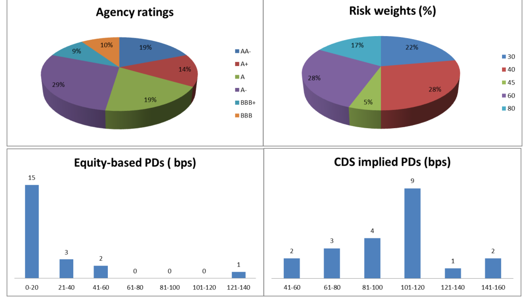
The breakdown of banks (as measured on 31/12/2014) by rating and risk weights is shown in the upper panels of Figure 1. The histograms in the lower panel of Figure 1 show the distribution by equity-based and CDSspread-implied PDs (again at year end 2014).
1 There are more complex ways of inferring an implied default probability from CDS spreads that (i) take account of the detailed cash flows of the CDS contract and (ii) attempt to strip out the risk premium in the spreads. For simplicity, we did not implement these more complex calculations.
The full results are shown in Table 2 which contains, for each bank, the four risk measures as measured at the end of 2008, 2010 2012 and 2014. Almost half the banks are either A or A- rated. Some A+ and AA banks are present. A small fraction of those included are either BBB+ or BBB rated.
About half the banks are on 30% or 40% risk weights using the lookup table in BCBS 307 that forms part of the proposed revision of the credit risk Standardised Approach. About another third have risk weights that are either 45% or 60% and just 17% of the bank exposures considered have 80% risk weights.
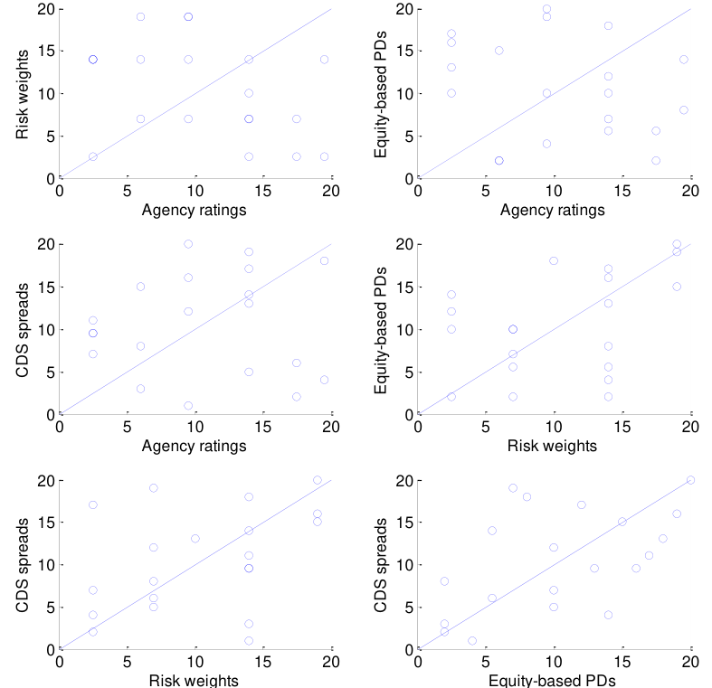
Table 2 shows the evolution of the different indicators in detail for each year end, bank by bank. (Figure 2 show the rank data graphically.) Several striking results emerge. Bank ratings have substantially more inertia than the other indicators, declining progressively over the period and showing no recovery in the latter years. In contrast, the market-based indicators indicate extreme credit risk at the end of 2008 just following the Lehman Brothers collapse. For North American banks, there is a steady and marked reduction in credit risk according to these indicators, especially in the equity-based measures. European banks show some recovery but with a temporary setback in 2012 reflecting the sovereign debt crisis in Europe in 2011-2012.
Table 3 shows rank correlations between the different risk indicators for end 2014. Rank correlations are calculated by assigning to each observation an integer rank for each of the underlying indicators and then calculating the correlation of the integer ranks. This approach tends to reveal how variables are related even when they are transformed in some nonlinear but monotonic way.
Very striking in Table 3 is the negative correlation between the order of bank credit quality implied by the agency ratings and the orders implied by the risk weights and equity-based PDs. The CDS spread implied PDs have a close to zero rank order correlation with agency ratings. The three non-rating indicators are all somewhat positively related as measured by the rank correlations although the correlation is no more than 51% (the rank correlation for the two market-data-based indicators).
Table 4 shows rank order correlations pooling data from each of the four year ends. (This yields 47 observations rather than the 20 available for the 2014 year end.) The negative relation between agency ratings and the other indicators is even more marked than for the end 2014 data. The correlations between the other three indicators are larger with CDS- and equity-implied PDs having a rank order correlation of 79%.
| Rating | Risk | Weight | (%) | PD | (bps) | CDS | (bps) | ||||||||||
|---|---|---|---|---|---|---|---|---|---|---|---|---|---|---|---|---|---|
| 2008 | 2010 | 2012 | 2014 | 2008 | 2010 | 2012 | 2014 | 2008 | 2010 | 2012 | 2014 | 2008 | 2010 | 2012 | 2014 | ||
| NATIONAL | AUSTRALIA BANK LTD | AA | AA | AA- | AA- | 60 | 384 | 103 | 56 | 26 | 105 | 105 | 61 | ||||
| AUST AND | NZ BANKING GROUP | AA | AA | AA- | AA- | 80 | 60 | 60 | 339 | 24 | 28 | 22 | 105 | 103 | 61 | ||
| COMERICA | INC | A | A- | A- | A- | 60 | 60 | 60 | 40 | 474 | 7 | 61 | 8 | 144 | 76 | 81 | 54 |
| WESTPAC | BANKING CORP | AA | AA | AA- | AA- | 60 | 60 | 142 | 44 | 19 | 16 | 105 | 105 | 61 | |||
| CREDIT | AGRICOLE SA | AA- | AA- | A | A | 100 | 80 | 398 | 151 | 312 | 45 | 163 | 167 | 71 | |||
| US BANCORP | AA | A+ | A+ | A+ | 100 | 60 | 60 | 40 | 37 | 19 | 8 | 1 | 161 | 76 | 60 | ||
| NATIONAL | BANK OF CANADA | A | A | A- | A | 60 | 178 | 6 | 5 | 2 | 68 | 72 | 51 | 41 | |||
| REGIONS | FINANCIAL CORP | A | BB+ | BBB- | BBB | 80 | 80 | 60 | 60 | 782 | 252 | 90 | 7 | 88 | |||
| BB&T CORP | A+ | A | A- | A- | 60 | 80 | 60 | 40 | 178 | 66 | 44 | 4 | 79 | 89 | |||
| JPMORGAN | CHASE & CO | A+ | A+ | A | A | 60 | 40 | 60 | 40 | 310 | 53 | 50 | 8 | 119 | 85 | 87 | 64 |
| KEYCORP | A- | BBB+ | BBB+ | BBB+ | 80 | 100 | 40 | 40 | 529 | 68 | 31 | 3 | 58 | ||||
| WELLS FARGO | & CO | AA | AA- | A+ | A+ | 300 | 80 | 60 | 60 | 243 | 30 | 17 | 1 | 105 | 77 | 48 | |
| PNC FINANCIAL | SERVICES GROUP | A+ | A | A- | A- | 60 | 60 | 60 | 473 | 32 | 40 | 3 | 68 | ||||
| BANK OF | AMERICA CORP | A+ | A | A- | A- | 100 | 60 | 60 | 45 | 569 | 240 | 206 | 27 | 177 | 130 | 67 | |
| AMERICAN | EXPRESS CO | A | BBB+ | BBB+ | BBB+ | 40 | 40 | 30 | 188 | 11 | 2 | 1 | 80 | 74 | 41 | ||
| CAPITAL ONE | FINANCIAL CORP | BBB+ | BBB | BBB | BBB | 60 | 40 | 30 | 529 | 210 | 129 | 19 | 264 | 125 | 94 | 49 | |
| BNP PARIBAS | AA+ | AA | A+ | A+ | 120 | 80 | 80 | 80 | 421 | 29 | 28 | 20 | 110 | 144 | 69 | ||
| UNITED | OVERSEAS BANK LTD | A+ | A+ | NR | AA- | 30 | 91 | 19 | 14 | 8 | 64 | 59 | |||||
| SOCIETE | GENERALE SA | AA- | A+ | A | A | 80 | 80 | 422 | 114 | 247 | 137 | 108 | 155 | 171 | 94 | ||
| CITIGROUP | INC | A | A | A- | A- | 300 | 40 | 30 | 30 | 925 | 86 | 93 | 10 | 185 | 144 | 127 | 74 |
| Agency ratings | 1.00 | -0.38 | -0.23 | 0.05 |
|---|---|---|---|---|
| Risk weights | -0.38 | 1.00 | 0.40 | 0.38 |
| Equity-based PDs | -0.23 | 0.40 | 1.00 | 0.51 |
| CDS spreads | 0.05 | 0.38 | 0.51 | 1.00 |
Note: 20 observations for each risk indicator
| Agency ratings | 1.00 | -0.48 | -0.09 | -0.12 |
|---|---|---|---|---|
| Risk weights | -0.48 | 1.00 | 0.45 | 0.49 |
| Equity-based PDs | -0.09 | 0.45 | 1.00 | 0.79 |
| CDS spreads | -0.12 | 0.49 | 0.79 | 1.00 |
Note: 47 observations for each risk indicator
4. Conclusion
What conclusions may one draw from the calculations presented above?
• Agency ratings cannot be ignored as measures of bank credit quality but they should be combined with other data sources
• Particularly since the crisis, bank ratings have appeared to show too much inertia
• In more normal times, agency ratings may be more reliable but in post crisis situations, their dynamics are questionable
• It is concerning that the rank order of ratings has recently been so little related to those of the other indicators
• The other measures are not fully convincing alternatives as they appear too volatile (equity-based measures), limited by illiquidity, availability and risk premia (CDS-based measures) and are not plausible discriminators of risk (in the case of risk weights)
• The lesson for investment institutions using credit risk indicators is that multiple indicators should be combined and used as inputs to internal rating processes
References
1. Basel Committee on Banking Supervision (2014a) “Capital Floors: The Design of a Framework Based on Standardised Approaches,” Consultative Document, December, (also known as BCBS 306), available at: http://www.bis.org/bcbs/publ/d306.pdf.
2. Basel Committee on Banking Supervision (2014b) “Revisions to the Standardised Approach for Credit Risk,” Consultative Document, December, (also known as BCBS 307), available at: http://www.bis.org/bcbs/publ/d307.pdf.
3. Hau, H., S. Langfield and D. Marques-Ibanez (2012) “Bank Ratings – What Determines Their Quality,” European Central Bnak Working Paper No. 1484, October, available at: https://www.ecb.europa.eu/pub/pdf/scpwps/ecbwp1484.pdf.
4. Merton, R. (1974) “On the pricing of corporate debt: the risk structure of interest rates,” Journal of Finance, 29, 449-470.
Appendix: Equity-based Default Probabilities
A.1. Modelling Approach To analyse the likelihood of default empirically, we develop a structural model of the bank’s equity. We start by assuming that the bank’s total underlying assets, denoted V, liabilities, D, and the market portfolio value, M, are described by the following set of geometric Brownian motions.
dVt = μvVtdt +σvVtdW[1]t (A1) dDt = μDDtdt (A2) dMt = μmMtdt +σmMtdW[2]t (A3)
. Here, we suppose that the correlation between asset and market portfolio is denoted ρ, i.e. dW[1]tdW[2]t = ρ dt We also assume that the bank’s earning flow is δ(Vt − Dt ) (with instantaneous dividend pay-out rate constant and equal to δ) and that the interest rate is constant and equal to r.
* * * It is immediate that the risk-adjusted drift term of V, D and M areμv = r −δ, μD = r −δ andμm = r . One can assume a logarithmic utility for a representative agent and derive the actual equilibrium drift terms as:
, and . μv = r −δ+σvσmρ μD = r −δ μm = r +σm
The above assumptions yield a parsimoniously expressed stochastic model of the evolution of the basic state variables. Given the processes V and D, by standard stochastic calculus, we can easily derive the process followed by the bank’s equity, X = X (V, D), which by no-arbitrage argument must satisfy:
σ * v 2 rX =δ(V − D) + μvVX v + μDDXD + V X vv 2 (A4)
Here, X v , X D and X vv denote the first derivative with respect to V, D and the second derivative with respect to V.
To derive the function X = X (V, D), we must lastly specify boundary conditions, namely under what conditions does bankruptcy occur. We suppose that insolvency takes place when the asset-liability ratio, denoted as k, falls below an exogenous trigger level. In our empirical work below, we assume that bankruptcy occurs at k levels equal to 0.95 or 1.00.
Using the homogeneity of equation (A5) and dividing quantities by liabilities D, we can find a simple solution to (rather than to ) where k = V / Dis defined to be the asset to liability ratio and Y(k) = X (k)1, X = X (V, D) Y(k) is the equity to liability ratio. Changing variables and by using appropriate boundary conditions ( limk→k Y(k) = 0 when insolvency occurs and limk→∞ Y(k) = k −1 when deposits become risk free), one obtains:
Y(k) = k −1− (k −1)(k / k)λ (A5)
2 4 2 σv / 2 − σv / 4 + 2σvδ with λ=[2] . (A6) σv
A.2. Statistical Implementation To implement the model statistically, we first calculate a time series of the ratio of equity market capitalisation to total liabilities for each company. While equity market capitalisation data is available daily, total liabilities data may be observed only quarterly, six monthly or annually depending on the firm. The annual data is sometimes not directly comparable to the more frequent observations since the former are audited. It is also desirable to follow a common approach for all firms.
We, therefore, base our analysis on the annual data, interpolating the annual observations using a cubic spline approach so as to obtain weekly observations. To bring the data up-to-date, we extrapolate the last annual observation using more recent quarterly or six monthly observations and then again perform an interpolation to obtain weekly observations to the present.
To estimate the parameters of the processes followed by each bank's asset-liability ratio, kt , Maximum Likelihood methods are employed. Three facts complicate the ML estimation. First, since our pricing expressions depend on the correlation parameter, ρ, we need to estimate a joint model of changes in kt and Mt .
Second, if the firm survives from t to t+Δ, kt must have remained above the insolvency trigger, k , in this interval of time. The likelihood is therefore constructed as the probability, conditional on observing kt and Mt , of (i) observing kt+Δ and Mt+Δ and (ii) that ks > k for all s∈[t,t + Δ]. The derivation of this density may be obtained from Risk Control. (The density for the univariate case is given in Cox and Miller (1973).)
Third, the equity-liability ratio will generally be a non-linear function, Y(kt ) of the asset-liability ratio, kt , and the function depends on the parameters of the kt process. In maximizing the likelihood, one must, therefore, for all the data points in the sample (which is, of course, computationally demanding) and multiply invert Y(.)
the density in the likelihood by a Jacobian adjustment term (because Yt is observed rather than kt ).
Having estimated the parameters for each bank's assets to liabilities ratio, one may invert Y(kt ) to obtain time series of the kt . Based on the level of kt at the end of the sample, various interesting quantities are calculated, including the value of implicit deposit insurance, the actuarially fair deposit insurance premium, and the probability of insolvency over different horizons.