

1. Introduction
This note presents a stress testing case study for a set of banks with inter-bank obligations, illustrating how stress testing may be accomplished using Risk Control’s Stress ControllerTM software. The calculations are performed for a banking sector comprising three individual banks (labelled A, B and C). The software may accommodate any number of banks and potentially other financial intermediaries.
We show how each bank’s balance sheet, P&L and key capital planning ratios are affected by macro scenarios including (i) a domestic country recession and (ii) a US recession. Note here that the “domestic country” is a notional small, open, emerging market economy. We also demonstrate (in scenario (iii)), how the software models a ‘contagion effect’ caused by the failure to fulfil inter-bank obligations resulting in a liquidity shock to one of the banks.
Changes in the credit quality of each bank’s loan book and fluctuations in the values of mark-to-market exposures affect the value of the banks’ balance-sheet items and the banks’ income through provisions and mark-to-market asset write-offs. A liquidity shortfall from a specific bank causes changes in that bank’s possible funding resources, as well as ‘inter-bank’ losses to other related banks resulting from inter-bank exposure insolvencies.
For a base case and for each of the stressed scenarios, predictions are supplied for the banks’ key variables. The results show how the impairment provisions rise and capital, asset growth, and profitability are depressed by the different recession scenarios. A US recession has a larger and more persistent impact than the domesticbased recession scenario.
The liquidity shock results also show that the rescue triggered by the liquidity shortfall increases the capital and funding of the distressed bank, as well as causing losses and capital reductions in the other banks.
Note that the framework described here may be used either with coarse, public data to perform high-level, topdown stress testing or with more granular internal data for bottom-up stress testing purposes. Financial statement modelling is highly flexible since equations may be written first in Excel, before being converted into scripts and then imported into the software for use at run-time to perform calculations.
2. Generating Consistent Macroeconomic Scenarios
To devise economic stress tests, one must generate consistent time paths for multiple macroeconomic variables. For example, to analyse the impact of a recession in the US on must model how such a recession affects macroeconomic variables in other countries and regions.
Risk Control’s Stress ControllerTM employs a statistical macroeconomic model in which users may specify shocks to particular variables and then calculate conditional forecasts of this and other variables. The statistical macroeconomic model is an example of the Global Vector Autoregressive or GVAR class of models. These have been widely used in economic forecasting and stress testing applications.
To allow for contagion between regions, GVAR models suppose that the vector of macroeconomic variables for a given region depends on its own lags and on weighted sums of variables form other regions.
The Stress ControllerTM GVAR model is flexible in that one may readily change the countries, regions and variables employed. In the exercise reported in this note, we employ as regions and countries the US, Europe excluding the UK, the UK, Asia and a set of emerging market countries including a mock country.
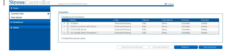
To create scenarios within Stress ControllerTM, the user may employ the web-based interface. Scenarios are stored within an underlying relational database and repeated calculations may be performed for a given scenario after amendments have been made to the scenario itself or after the underlying data has been updated. Figure 1 shows the list of scenarios within the Stress ControllerTM web-based interface.
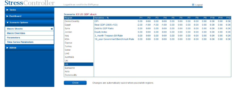
Figure 2 provides a screenshot of the software, illustrating how one may edit a scenario. In this case, the scenario consists of a sequence of period-by-period shocks to macroeconomic variables. Non-interest-rate macro time series are stored in log form times 100. Hence, a shock of negative one unit in a given quarter to a scenario variable such as GDP corresponds to a minus 1% innovation.
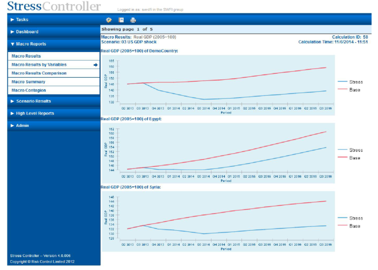
Stress ControllerTM produces time paths of macroeconomic variables such as those shown in Figure 3. These time series are the mean values of the variables in question conditional on the assumed shocks to the scenario variables.
a scenario in the form of a set of time series for different macroeconomic variables. Hence, one may work with scenarios generated by regulators or a bank’s economics department, importing the scenario time series into the application and then performing additional calculations with them.
In this study we interpolate the IMF World Economic Outlook released in October 2013 into a series of quarterly forecasts for the following 12 quarters and then employ them as our baseline results.
Note that, as an alternative to generating macroeconomic scenarios within Stress ControllerTM, one may import
3. Loan Portfolio Modelling
One may model loans within Stress ControllerTM either as individual rated exposures or as diversified pool exposures with a default rate that evolves over time. For the exercise reported in this paper, we use diversified pool exposures.
In separate publications, we show how to derive simple but rigorous models of the dynamic behaviour of loss rates on pools of homogeneous loans. These may be modelled unconditionally or conditional on macroeconomic variables. In the latter case, the default rate evolves as an auto-correlated time series driven by shocks to macro variables like GDP, interest rates or unemployment.
The sensitivities to the shocks are sector-specific and asset-class-specific. We have obtained estimates in a series of past studies of the macroeconomic impact on loan books using data from different banks and a range of public data sources. In this study, we have calibrated the sensitivities to be bank-specific to show how different banks react differently to the same recession.
4. Modelling Financial Statements
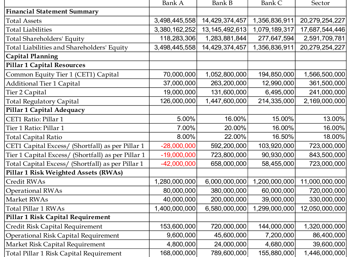
The Three Banks The banking sector created for this case study consists of 3 individual banks. Stress testing is performed for each of the banks and for the sector as a whole. The initial assets size and capital ratio for each of the banks and for the sector are summarized in Figure 4, below.
Modelling the Bank’s Balance Sheet For each individual bank, the financial and capital planning is treated as Balance Sheet driven. Both assets and liabilities depend on the forecasts of macro variables, provision calculations and on user-defined parameters. The Income Statement calculations rely mainly on the forecasted Balance Sheet variables.
At the sector level, the model allows the user to apply shocks to individual banks and to monitor the possibility of a liquidity shortfall and its associated contagion effects. The order of the calculations within each period is as follows:
For each bank:
(1) Risk factor driven BS items;
(2) Other BS items that are either dependent upon the risk factor driven items or are relatively stable over time;
(3) Off BS items;
(4) Income Statement (IS) items that are calculated based on the forecasted BS;
(5) Shareholder equity BS items, which take into account IS forecasts;
(6) Balancing the BS;
(7) Liquidity surplus/shortfall result;
After the above calculations are complete for each bank, the model starts another round of calculations for each bank:
(1) Inter-subsidiary contagion effect;
(2) Surplus/shortfall adjustments to BS and IS items
(3) Recalculating the BS and IS;
(4) Re-balancing the BS;
After the above calculations for each bank are completed, the model starts another round of calculations for each bank:
(1) ICAAP items
(2) Other report items
Finally, the model performs sector consolidation, sector ICAAP and report items calculations. The key assumptions we make in modelling the financial statements and capital planning are as follows.
1. We view the individual bank’s financial and capital planning as balance-sheet driven, and the sector result as driven by the results of individual banks.
2. For each individual bank, the risk factor driven balance sheet items are modelled first. Loans, investment portfolio and deposits are the most obvious risk factor driven balance-sheet items and they are assumed to be affected by the macro-economy. The asset side is also affected through the impact of macro shocks on provisions and changes in mark-to-market values.
3. Other balance sheet items are either dependent upon the risk factor driven items or are relatively stable over time.
4. Loans and deposits are assumed to be linked to (a) GDP growth in the relevant region, and (b) userdefined growth rate overrides. The relative importance of (a) and (b) and the sensitivity to macro shocks vary for different loans and deposits. The approach employed in this case study could be generalized to include interest rates or other macroeconomic variables such as unemployment rates but we have preferred in this exercise to keep the analysis as simple as possible.
5. Marked-to-market assets and liabilities are assumed to be sensitive to relevant macro indicators, in particular to GDP or national equity indices.
delled based on the forecasted balance sheet. Interest related items are
6. The Income Statement is mod calculated based on (a) interest-generating and interest-bearing items from forecasted balance sheet and (b) user-defined rate shocks.
7. The credit impairment charge is calculated as the expected losses of loans and advances to retail and wholesale customers, taking into account the lagged impact of macroeconomic variables on provisions.
8. To balance the financial position statement at the end of each forecasting period, we adjust the gap between forecast ‘Total Assets’ and ‘Total Liabilities and Shareholder Equities’, allowing this gap to be absorbed by multiple items employing user-defined weights.
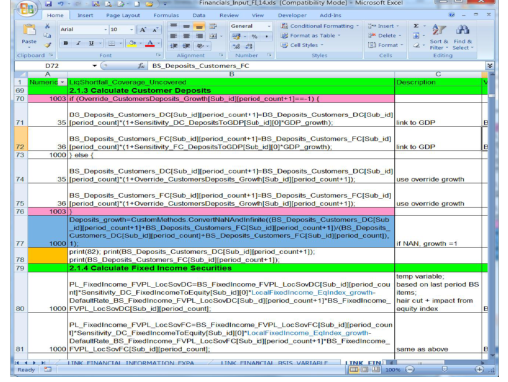
The equations for the financial statements analysis are treated in Stress ControllerTM as part of the model’s data. They are imported from a ‘feeder’ Excel workbook. A screenshot of the equations stored in such a workbook is provided in Figure 5.
Before the equations are executed, all the variables employed in the equation must be declared by importing a workbook containing the definition of each variable.
Note: All values are expressed in 1,000 of
5. Results
Using the approach described above, we perform an analysis of the impact of several stress scenarios on the banks’ financial and capital planning. Below, we present results for (i) a base case (i.e., an unconditional forecast), (ii) a domestic country recession, (iii) a US recession and (iv) a liquidity shock to one of the banks.
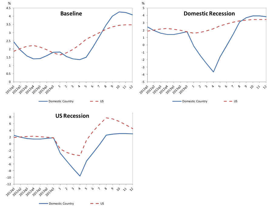
Recession Scenarios The recession scenarios consist of a sequence of shocks to real GDP in the geographic region in question. In both cases, the shocks are -2% in Q1 and -1% in Q2, Q3 and Q4. These shocks sum to a cumulative negative shock of 5% over 1 year. Conditional on a set of negative shocks to a specific region’s GDP, the model generates forecasts of all other macroeconomic variables including the GDP in other regions and market prices, including equity indices and interest rates by region.
We perform the analysis from the perspective of information available at the end of Quarter 3 of 2013. As mentioned earlier, the software allows the user either to forecast the baseline from historical data or to construct the baseline by importing a set of time series forecasts. In this study, we interpolate the IMF World Economic Outlook released in October 2013 into a series of quarterly forecasts for the following 12 quarters and employ them as our baseline results.
Figure 6 shows the effects of the base case and the 2 recession scenarios on GDP growth rates in different regions. We also include the historical growth rates from the beginning of 2012. One can see that the US Recession has a larger cumulative impact on domestic country GDP growth than do the shocks associated with the local recession scenario. At the end of Q4 the year-to-year real GDP growth rate of the domestic country is - 10% in the US recession scenario whereas it is only -4% in the domestic country recession. This reflects the fact that in our calibration the domestic country is a small, open, emerging market economy.
Figure 7 shows the time paths of US GDP under the baseline and US recession scenarios. One can see that the stressed result reverts after the shocks (i.e., after Q3 2014) and then converges to the baseline result. This recovery from shocks makes US GDP experience fast year-to-year growth, clearly visible in the ‘US Recession’ section in Figure 6. However, it can be seen in Figure 7 that US GDP has still not reached the baseline level by the end of the observed period.
Figure 7: Screenshot of US Recession scenario (Stress) Result
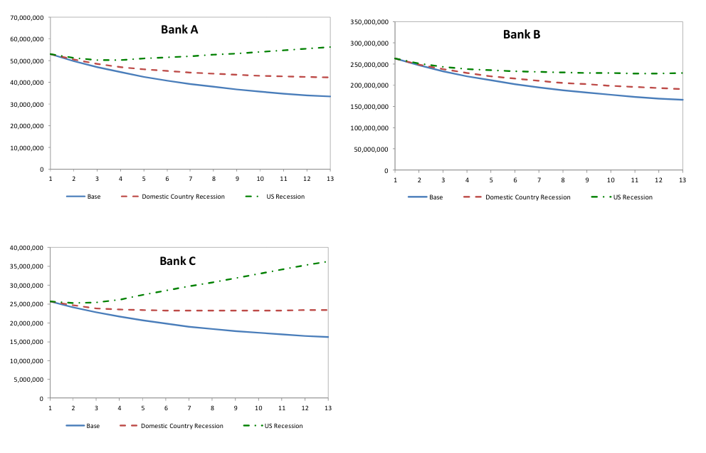
Within the model, the recession scenarios have impacts on the credit quality of the banks’ counter-parties and hence boost the credit impairment provisions of the banks’ loans, as shown in Figure 8. As one may observe, for all three banks, the impairment provisions are downward sloping in the baseline scenario but rise significantly away from the base case level in the US recession scenario. The increase in the domestic recession scenario’s provisions is of smaller magnitude than that of the US recession scenario, showing that the US recession has a stronger effect on the credit quality of the banks’ loans.
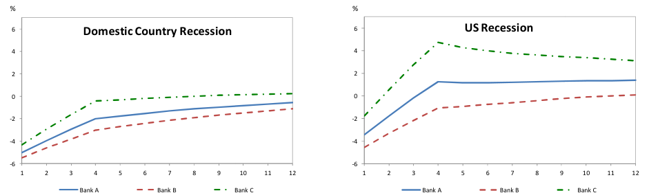
One may note that the three banks’ credit impairment provisions exhibit different sensitivities to the recessions, with Bank C appearing to be the most sensitive and Bank B the least. This observation is clearly illustrated in Figure 9, where we compare the credit impairment provision growth rates of different banks under the same scenario. One may observe that in both recessions the highest growth rate is that of Bank C and the lowest that of Bank B. The growth rates in the US recession scenario are in general larger than that in the domestic recession case.
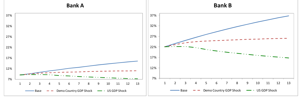
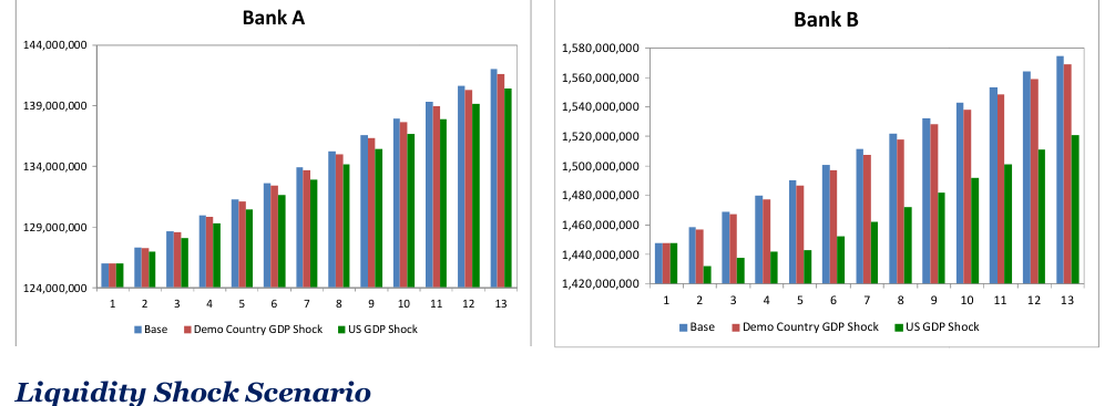
In Figures 10 and 11 we show the impact of the recession scenarios on the individual banks’ capital planning. One may note that the decrease in capital ratio and total regulatory capital is more significant in Bank B than that in Bank A. This reflects the fact that Bank B has a much more ‘loan dominated’ financial statements (‘Loans’ relative to ‘Total Assets’ and ‘Impairment Charge’ relative to ‘Net Profits’).
In the liquidity shock scenario, we assume there is significant funding run-off in Q1 for Bank A, which results in a liquidity shortfall for that subsidiary in that period.
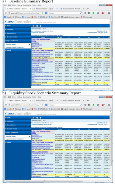
Figure 12 shows screenshots from the overall banking sector summary report under baseline and liquidity shock scenarios, where one can see that at the sector level, a liquidity shortfall in Q1 in the liquidity shock scenario is reported. (We only report results at the sector level in this note but all individual banks’ results can be viewed from the software’s interface).
Within the model, if any bank experiences a liquidity shortfall, a ‘rescue’ process will be triggered. In this ‘rescue’ process, the shortfall is covered by different funding sources, including:(1) a loan from the central bank and other banks, (2) capital injection from shareholders, and then finally (3) the remaining shortfall will be covered by the related banks by reducing the problematic bank’s inter-bank obligations.
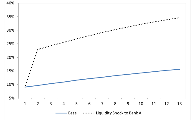
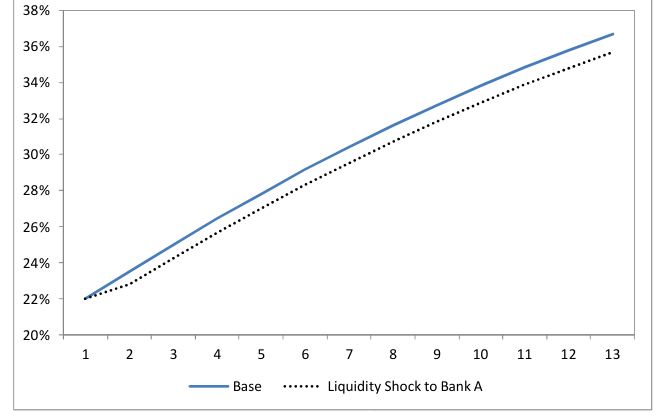
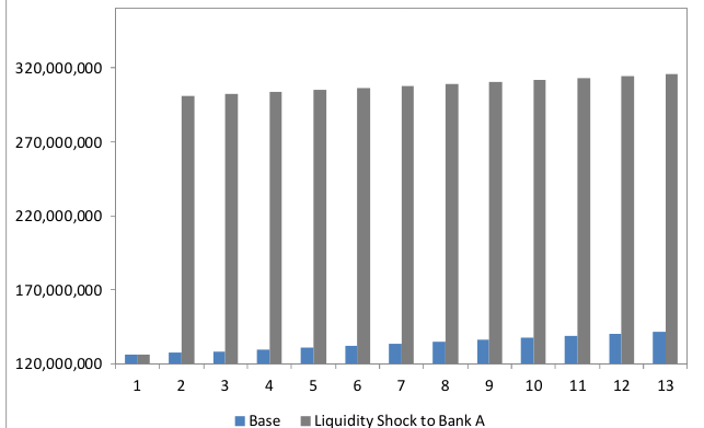
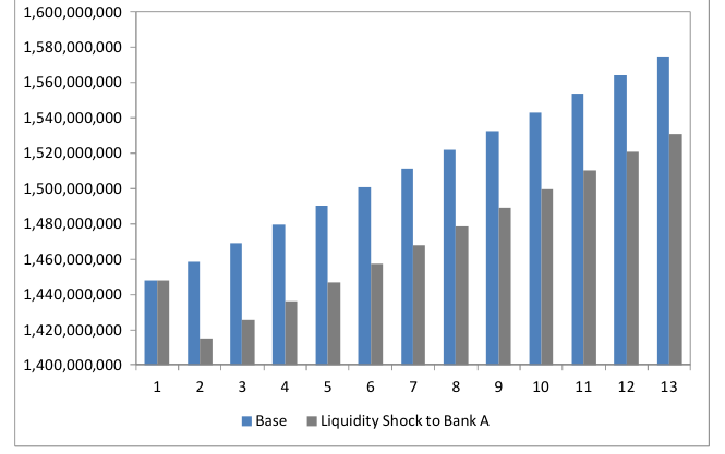
Due to both the rescue of the problematic bank and loss sharing between the related banks, one would expect the capital to increase for the problematic bank and to decrease for the related banks. Figures 11 to 14 show the results for Bank A and B.
6. Conclusion
The analysis in this note illustrates how Stress ControllerTM may be used to stress test a group of related banks. It is straightforward to change the logic of the modelling to accommodate quite different forms of analysis.
For example, one may include, as an input to the calculations, a central-case projection of the financial statements for each reporting entity and then model deviations from that base case as driven by shocks to macroeconomic and market variables.
Such an approach renders the analysis consistent with a set of projections generated by, for example, a forecasting function, while permitting the risk function to investigate the impact of a set of stress scenarios on the banking sector.
To this extent, Stress ControllerTM is an environment within which a wide range of company and sector specific financial statement and capital projections may be performed.
Risk Control Limited 13-14 Dean Street London W1D 3RS UK T: +44 (0)203 307 0730
www.riskcontrollimited.com