This paper generalizes a class of ratings-based credit derivative models proposed by Jarrow, Lando, and Turnbull (1997) and Kijima and Komoribayashi (1998) to allow for stochastic spreads and then applies this model to analyze empirically the pricing of large cross sections of corporate bonds and Asset Backed Securities. We show that measuring risk in credit portfolios is highly sensitive to the inclusion of randomness in spreads.
1 Introduction of credit spreads. As conditional probabilities, these evolve as martingale pro- \text{of credit spreads. As conditional probabilities, these evolve as martingale pro-} of credit spreads. As conditional probabilities, these evolve as martingale pro- from large cross sections of corporate bond and Asset Backed Security (ABS) \text{from large cross sections of corporate bond and Asset Backed Security (ABS)} from large cross sections of corporate bond and Asset Backed Security (ABS) ranges are more or less correlated with other parts of the market. Second, it \text{ranges are more or less correlated with other parts of the market. Second, it} ranges are more or less correlated with other parts of the market. Second, it in financial institutions. It is interesting to quantify how much the introduction \text{in financial institutions. It is interesting to quantify how much the introduction} in financial institutions. It is interesting to quantify how much the introduction 2.1 Notation matrix for each future period is the historical matrix with probability shifted off \text{matrix for each future period is the historical matrix with probability shifted off} matrix for each future period is the historical matrix with probability shifted off assume that shocks to the interest rates and those to credit risk are independent. \text{assume that shocks to the interest rates and those to credit risk are independent.} assume that shocks to the interest rates and those to credit risk are independent. exp [ S t , j ( k ) j ] = P r o b t ∗ ( τ d > t + j ∣ k ) + γ [ 1 − P r o b t ∗ ( τ d > t + j ∣ k ) ] \exp\left[S_{t,j}^{(k)} j\right] = \mathrm{Prob}_{\mathrm{t}}^{*}\left(\tau^{\mathrm{d}} > \mathrm{t}+\mathrm{j}|\mathrm{k}\right) + \gamma\left[1 - \mathrm{Prob}_{\mathrm{t}}^{*}\left(\tau^{\mathrm{d}} > \mathrm{t}+\mathrm{j}|\mathrm{k}\right)\right] exp [ S t , j ( k ) j ] = Prob t ∗ ( τ d > t + j ∣ k ) + γ [ 1 − Prob t ∗ ( τ d > t + j ∣ k ) ] (1) Here, Prob t ∗ ( . ) denotes the risk-adjusted probability conditional on information at date t . Also, τ d is the random time at which default occurs. Let Q t , j ( k ) denote \text{Here, Prob}^{*}_{\mathrm{t}}(.) \text{ denotes the risk-adjusted probability conditional on information at date } t. \text{ Also, } \tau^{d} \text{ is the random time at which default occurs. Let } Q^{(k)}_{t,j} \text{ denote} Here, Prob t ∗ ( . ) denotes the risk-adjusted probability conditional on information at date t . Also, τ d is the random time at which default occurs. Let Q t , j ( k ) denote Then: Q t , j ( k ) ≡ P r o b ( τ ∗ ∈ { t , t + 1 , . . . , t + j } ) = 1 − exp [ − S t , j ( k ) j ] 1 − γ \text{Then:}\quad Q_{t,j}^{(k)} \equiv \mathrm{Prob}\left(\tau^{*} \in \{\mathrm{t}, \mathrm{t}+1, ..., \mathrm{t}+\mathrm{j}\}\right) = \frac{1 - \exp[-\mathrm{S}_{\mathrm{t,j}}^{(\mathrm{k})}\mathrm{j}]}{1 - \gamma} Then: Q t , j ( k ) ≡ Prob ( τ ∗ ∈ { t , t + 1 , ... , t + j } ) = 1 − γ 1 − exp [ − S t , j ( k ) j ] (2) Let q t , j ( k ) be the probability that default occur between t+j-1 and t+j conditional on information at t and in particular conditional on the fact that the exposure \text{Let } q^{(k)}_{t,j} \text{ be the probability that default occur between t+j-1 and t+j conditional on information at } t \text{ and in particular conditional on the fact that the exposure} Let q t , j ( k ) be the probability that default occur between t+j-1 and t+j conditional on information at t and in particular conditional on the fact that the exposure q t , j ( k ) = P r o b t ( τ d = t + j ∣ rating at t = k ) = Q t , j ( k ) − Q t , j − 1 ( k ) . q_{t,j}^{(k)} = \mathrm{Prob}_{\mathrm{t}}(\tau^{\mathrm{d}} = \mathrm{t}+\mathrm{j}|\text{rating at t } = \mathrm{k}) = \mathrm{Q}_{\mathrm{t,j}}^{(\mathrm{k})} - \mathrm{Q}_{\mathrm{t,j-1}}^{(\mathrm{k})}. q t , j ( k ) = Prob t ( τ d = t + j ∣ rating at t = k ) = Q t , j ( k ) − Q t , j − 1 ( k ) . (3) The probabilities for different ratings are denoted q t , j ( k ) ≡ [ q t , j ( 1 ) , q t , j ( 2 ) , … , q t , j ( N ) ] . \text{The probabilities for different ratings are denoted } q^{(k)}_{t,j} \equiv \left[ q^{(1)}_{t,j}, q^{(2)}_{t,j}, \ldots, q^{(N)}_{t,j} \right]. The probabilities for different ratings are denoted q t , j ( k ) ≡ [ q t , j ( 1 ) , q t , j ( 2 ) , … , q t , j ( N ) ] . 2.2 Structure of the Transition Matrices matrices M t , 1 , M t , 2 , … . The ( k , l ) th element of M t , j represents the probability \text{matrices } M_{t,1}, M_{t,2}, \ldots. \text{ The } (k,l)\text{th element of } M_{t,j} \text{ represents the probability} matrices M t , 1 , M t , 2 , … . The ( k , l ) th element of M t , j represents the probability M t , j = [ M t , j ( − d ) ⋮ M t , j ( d ) … … … … 0 ⋮ 1 ] . M_{t,j} = \left[\begin{array}{ccc} M_{t,j}^{(-d)} & \vdots & M_{t,j}^{(d)} \\ \ldots & \ldots \ \ldots & \ldots \\ 0 & \vdots & 1 \end{array}\right]. M t , j = M t , j ( − d ) … 0 ⋮ … … ⋮ M t , j ( d ) … 1 . (4) Where M t , j ( − d ) is N × N and M t , j ( d ) is N × 1. For any M dimensional vector v , \text{Where } M^{(-d)}_{t,j} \text{ is } N \times N \text{ and } M^{(d)}_{t,j} \text{ is } N \times 1. \text{ For any } M \text{ dimensional vector } v, Where M t , j ( − d ) is N × N and M t , j ( d ) is N × 1. For any M dimensional vector v , adopt the notation: I ( v ) = [ v 1 0 … 0 0 v 2 … 0 ⋮ ⋮ ⋱ ⋮ 0 … 0 v M ] \text{adopt the notation: } I(v) = \begin{bmatrix} v_1 & 0 & \ldots & 0 \\ 0 & v_2 & \ldots & 0 \\ \vdots & \vdots & \ddots & \vdots \\ 0 & \ldots & 0 & v_M \end{bmatrix} adopt the notation: I ( v ) = v 1 0 ⋮ 0 0 v 2 ⋮ … … … ⋱ 0 0 0 ⋮ v M (5) is an N × N diagonal matrix for any N − vector v = ( v 1 , v 2 , . . . , v N ) ′ . \text{is an } N \times N \text{ diagonal matrix for any } N-\text{vector } v = (v_1, v_2, ..., v_N)'. is an N × N diagonal matrix for any N − vector v = ( v 1 , v 2 , ... , v N ) ′ . Assumption 1 Now, suppose M t , j ( − d ) M_{t,j}^{(-d)} M t , j ( − d )
M t , j ( − d ) ≡ I ( 1 N − M t , j ( d ) ) M ~ M^{(-d)}_{t,j} \equiv I(1_N - M^{(d)}_{t,j})\tilde{M} M t , j ( − d ) ≡ I ( 1 N − M t , j ( d ) ) M ~ (6) where M ~ is invertible. \textit{where } \tilde{M} \textit{ is invertible.} where M ~ is invertible. Here, note that M ~ is time homogenous and may be interpreted as the rating \text{Here, note that } \tilde{M} \text{ is time homogenous and may be interpreted as the rating} Here, note that M ~ is time homogenous and may be interpreted as the rating Proposition 1 Under Assumption 1, one may derive an explicit expression for the forward default probabilities conditional on information at t t t
M t , 1 ( d ) = 1 1 − γ [ 1 − exp [ − S t , 1 ( 1 ) ( j ) ] ⋮ 1 − exp [ − S t , 1 ( N ) ( j ) ] ] M^{(d)}_{t,1} = \frac{1}{1-\gamma} \begin{bmatrix} 1 - \exp[-S^{(1)}_{t,1}(j)] \\ \vdots \\ 1 - \exp[-S^{(N)}_{t,1}(j)] \end{bmatrix} M t , 1 ( d ) = 1 − γ 1 1 − exp [ − S t , 1 ( 1 ) ( j )] ⋮ 1 − exp [ − S t , 1 ( N ) ( j )] (7) M t , j ( d ) = 1 1 − γ ∏ k = 1 j − 1 ( I ( 1 N − M t , k ( d ) ) M ~ ) − 1 [ exp [ − S t , j − 1 ( 1 ) ( j − 1 ) ] − exp [ − S t , j ( 1 ) ( j ) ] ⋮ exp [ − S t , j − 1 ( N ) ( j − 1 ) ] − exp [ − S t , j ( N ) ( j ) ] ] M_{t,j}^{(d)} = \frac{1}{1-\gamma} \prod_{k=1}^{j-1} \left( I(1_N - M_{t,k}^{(d)}) \tilde{M} \right)^{-1} \left[ \begin{array}{c} \exp[-S_{t,j-1}^{(1)}(j-1)] - \exp[-S_{t,j}^{(1)}(j)] \\ \vdots \\ \exp[-S_{t,j-1}^{(N)}(j-1)] - \exp[-S_{t,j}^{(N)}(j)] \end{array} \right] M t , j ( d ) = 1 − γ 1 k = 1 ∏ j − 1 ( I ( 1 N − M t , k ( d ) ) M ~ ) − 1 exp [ − S t , j − 1 ( 1 ) ( j − 1 )] − exp [ − S t , j ( 1 ) ( j )] ⋮ exp [ − S t , j − 1 ( N ) ( j − 1 )] − exp [ − S t , j ( N ) ( j )] exp[−St,j(N−)[1](j − 1)] − exp[−St,j(N)(j)]
for j = 2 , 3 , … , \text{for } j = 2, 3, \ldots, for j = 2 , 3 , … , Conversely, the spreads S t , j ( n ) S_{t,j}^{(n)} S t , j ( n ) M t , j ( d ) M_{t,j}^{(d)} M t , j ( d )
2.3 Fitting Observed Spreads The above model provides a consistent set of risk-adjusted distributions for fu- \text{The above model provides a consistent set of risk-adjusted distributions for fu-} The above model provides a consistent set of risk-adjusted distributions for fu- benchmark the distributions from a single cross section of spreads observed at date t ( S t , j ( n ) for j = 1 , 2 , … and n = 1 , 2 , … , N ) by choosing the M t , j ( d ) appropri- \text{benchmark the distributions from a single cross section of spreads observed at date } t \ (S_{t,j}^{(n)} \text{ for } j = 1, 2, \ldots \text{ and } n = 1, 2, \ldots, N) \text{ by choosing the } M_{t,j}^{(d)} \text{ appropri-} benchmark the distributions from a single cross section of spreads observed at date t ( S t , j ( n ) for j = 1 , 2 , … and n = 1 , 2 , … , N ) by choosing the M t , j ( d ) appropri- the forward default probability for one rating k may be lower than that for a \text{the forward default probability for one rating } k \text{ may be lower than that for a} the forward default probability for one rating k may be lower than that for a min M t , j ( d ) ∑ [ S t , j ( n ) − h ( { M t , j ( d ) , j = 1 , 2 , … , J , n = 1 , … , N } ) ] 2 \min_{M_{t,j}^{(d)}} \sum \left[ S_{t,j}^{(n)} - h\left( \left\{ M_{t,j}^{(d)} \ , \ j = 1, 2, \ldots, J \ , \ n = 1, \ldots, N \right\} \right) \right]^2 M t , j ( d ) min ∑ [ S t , j ( n ) − h ( { M t , j ( d ) , j = 1 , 2 , … , J , n = 1 , … , N } ) ] 2 j = 1, . . . , J j = 1, 2, . . . n = 1, . . . N n = 1, . . . , N
subject to M t , j , n ( d ) > M t , j , n + 1 ( d ) for all j = 1 , 2 , … n = 1 , … , N − 1 . \text{subject to } M_{t,j,n}^{(d)} > M_{t,j,n+1}^{(d)} \text{ for all } j = 1, 2, \ldots \quad n = 1, \ldots, N-1 \ . subject to M t , j , n ( d ) > M t , j , n + 1 ( d ) for all j = 1 , 2 , … n = 1 , … , N − 1 . (8) Here, h ( . ) is the mapping from the M t , j ( d ) to the S t , j implied by the inverse of the \text{Here, } h(.) \text{ is the mapping from the } M_{t,j}^{(d)} \text{ to the } S_{t,j} \text{ implied by the inverse of the} Here, h ( . ) is the mapping from the M t , j ( d ) to the S t , j implied by the inverse of the fully predictable at some initial date 0. To see how spreads will vary, note that \text{fully predictable at some initial date } 0. \text{ To see how spreads will vary, note that} fully predictable at some initial date 0. To see how spreads will vary, note that [ M t , 1 ( − d ) M t , 1 ( d ) 0 N ′ 1 ] , [ M t , 2 ( − d ) M t , 2 ( d ) 0 N ′ 1 ] , ⋯ , [ M t , j − 1 ( − d ) M t , j − 1 ( d ) 0 N ′ 1 ] , [ M t , j ( − d ) M ] \left[ \begin{array}{cc} M_{t,1}^{(-d)} & M_{t,1}^{(d)} \\ 0_N' & 1 \end{array} \right] , \left[ \begin{array}{cc} M_{t,2}^{(-d)} & M_{t,2}^{(d)} \\ 0_N' & 1 \end{array} \right] , \ \cdots \ , \left[ \begin{array}{cc} M_{t,j-1}^{(-d)} & M_{t,j-1}^{(d)} \\ 0_N' & 1 \end{array} \right] , \left[ \begin{array}{cc} M_{t,j}^{(-d)} & M \end{array} \right] [ M t , 1 ( − d ) 0 N ′ M t , 1 ( d ) 1 ] , [ M t , 2 ( − d ) 0 N ′ M t , 2 ( d ) 1 ] , ⋯ , [ M t , j − 1 ( − d ) 0 N ′ M t , j − 1 ( d ) 1 ] , [ M t , j ( − d ) M ] (9) j − 2 , the two year spreads will be determined by the product of the last two j-2, \text{ the two year spreads will be determined by the product of the last two} j − 2 , the two year spreads will be determined by the product of the last two One may deduce the following proposition: \text{One may deduce the following proposition:} One may deduce the following proposition: Proposition 2 Under Assumption 1, spreads S t , j ( n ) S_{t,j}^{(n)} S t , j ( n ) n = 1 , 2 , … , N n = 1, 2, \ldots, N n = 1 , 2 , … , N j = 1 , 2 , … j = 1, 2, \ldots j = 1 , 2 , … t = 1 , 2 , … t = 1, 2, \ldots t = 1 , 2 , …
forward default probabilities are constant over time for any given j j j
M t 1 , j ( d ) = M t 2 , j ( d ) M_{t_1,j}^{(d)} = M_{t_2,j}^{(d)} M t 1 , j ( d ) = M t 2 , j ( d ) (10) for all t 1 and t 2 . \textit{for all } t_1 \textit{ and } t_2. for all t 1 and t 2 . 2.4 Stochastic Spreads in M t , j , d implies evolution in the risk adjusted transition matrices that market \text{in } M_{t,j,d} \text{ implies evolution in the risk adjusted transition matrices that market} in M t , j , d implies evolution in the risk adjusted transition matrices that market probabilities increase as the credit quality decreases. A simple way to ensure this \text{probabilities increase as the credit quality decreases. A simple way to ensure this} probabilities increase as the credit quality decreases. A simple way to ensure this [ M t + 1 , j − 1 , d 1 M t + 1 , j − 1 , d 2 ⋮ M t + 1 , j − 1 , d N ] = η t + 1 , j − 1 [ M t , j , d 1 M t , j , d 2 ⋮ M t , j , d N ] \left[\begin{array}{c} M^{1}_{t+1,j-1,d} \\ M^{2}_{t+1,j-1,d} \\ \vdots \\ M^{N}_{t+1,j-1,d} \end{array}\right] = \eta_{t+1,j-1} \left[\begin{array}{c} M^{1}_{t,j,d} \\ M^{2}_{t,j,d} \\ \vdots \\ M^{N}_{t,j,d} \end{array}\right] M t + 1 , j − 1 , d 1 M t + 1 , j − 1 , d 2 ⋮ M t + 1 , j − 1 , d N = η t + 1 , j − 1 M t , j , d 1 M t , j , d 2 ⋮ M t , j , d N (11) where η t + 1 , j − 1 is a common shock affecting all rating categories for a particular \text{where } \eta_{t+1,j-1} \text{ is a common shock affecting all rating categories for a particular} where η t + 1 , j − 1 is a common shock affecting all rating categories for a particular E t ( η t + 1 , j − 1 ) = 1 for all t , j . E_t(\eta_{t+1,j-1}) = 1 \ \text{ for all } t, j. E t ( η t + 1 , j − 1 ) = 1 for all t , j . (12) 3 Empirical Implementation 4.2 Extracting Forward Default Probabilities 4.3 Volatilities and Correlations picture is one of smooth decline in correlation as distance in maturity grows. This \text{picture is one of smooth decline in correlation as distance in maturity grows. This} picture is one of smooth decline in correlation as distance in maturity grows. This resents 46% of the eigenvalue sum. Two other eigenvalues are quite large in this \text{resents 46\% of the eigenvalue sum. Two other eigenvalues are quite large in this} resents 46% of the eigenvalue sum. Two other eigenvalues are quite large in this three substantial eigenvalues suggesting no simple factor structure. The eigen- \text{three substantial eigenvalues suggesting no simple factor structure. The eigen-} three substantial eigenvalues suggesting no simple factor structure. The eigen- 4.4 Expected Returns and Risk Premia years after the start of the sample). While the forward default probabilities should \text{years after the start of the sample). While the forward default probabilities should} years after the start of the sample). While the forward default probabilities should -6.6 over the 4 years of the sample period. In other words, the downward drift in \text{-6.6 over the 4 years of the sample period. In other words, the downward drift in} -6.6 over the 4 years of the sample period. In other words, the downward drift in This decline may be interpreted as the decline required to compensate agents \text{This decline may be interpreted as the decline required to compensate agents} This decline may be interpreted as the decline required to compensate agents for holding claims with spread risk, i.e., it is reflective of the spread-volatility risk \text{for holding claims with spread risk, i.e., it is reflective of the spread-volatility risk} for holding claims with spread risk, i.e., it is reflective of the spread-volatility risk 5 Portfolio Value Simulations to explore the economic significance of them in a portfolio context. In this section, \text{to explore the economic significance of them in a portfolio context. In this section,} to explore the economic significance of them in a portfolio context. In this section, maximum bond position face value is less than double the average value. The \text{maximum bond position face value is less than double the average value. The} maximum bond position face value is less than double the average value. The framework described in Section 2 except that correlation between rating transi- \text{framework described in Section 2 except that correlation between rating transi-} framework described in Section 2 except that correlation between rating transi- stochastic spreads with normal mixture shocks. The normal mixture shocks are \text{stochastic spreads with normal mixture shocks. The normal mixture shocks are} stochastic spreads with normal mixture shocks. The normal mixture shocks are sitive in the Gaussian case, especially in the case of the longer, 1-year holding \text{sitive in the Gaussian case, especially in the case of the longer, 1-year holding} sitive in the Gaussian case, especially in the case of the longer, 1-year holding 6 Conclusion ratings-based pricing model building on earlier contributions by Jarrow, Lando, \text{ratings-based pricing model building on earlier contributions by Jarrow, Lando,} ratings-based pricing model building on earlier contributions by Jarrow, Lando, abilities. Our results suggest there is a risk premium on spread risk and we doc- \text{abilities. Our results suggest there is a risk premium on spread risk and we doc-} abilities. Our results suggest there is a risk premium on spread risk and we doc- 7 Appendix A: Derivations 8 Appendix B: Term Structure Fitting Algo- rithm (2007). These involve fitting the bond prices using a time-homogeneous, risk- \text{(2007). These involve fitting the bond prices using a time-homogeneous, risk-} (2007). These involve fitting the bond prices using a time-homogeneous, risk- number of years. Maintainting the original yield to maturity, we then calculate \text{number of years. Maintainting the original yield to maturity, we then calculate} number of years. Maintainting the original yield to maturity, we then calculate sition matrix. We parameterize a tri-diagonal matrix quarterly transition \text{sition matrix. We parameterize a tri-diagonal matrix quarterly transition} sition matrix. We parameterize a tri-diagonal matrix quarterly transition 2. We then calculate the annual transition matrix, by taking the triangular \text{2. We then calculate the annual transition matrix, by taking the triangular} 2. We then calculate the annual transition matrix, by taking the triangular are equal to the right-hand column of the j power of the annual transition \text{are equal to the right-hand column of the j power of the annual transition} are equal to the right-hand column of the j power of the annual transition 4. We price the bonds. We assume that the mean recovery rate is 50 \text{4. We price the bonds. We assume that the mean recovery rate is 50} 4. We price the bonds. We assume that the mean recovery rate is 50 the maximum number of 2,000 iterations is exceeded, we report the vector \text{the maximum number of 2,000 iterations is exceeded, we report the vector} the maximum number of 2,000 iterations is exceeded, we report the vector References de Jong, F., and J. Driessen (2006): “Liquidity Risk Premia in Corporate \text{de Jong, F., and J. Driessen (2006): ``Liquidity Risk Premia in Corporate} de Jong, F., and J. Driessen (2006): “Liquidity Risk Premia in Corporate Spreads: Default, Recovery, Tax, Jumps, Liquidity, and Market Factors,” \text{Spreads: Default, Recovery, Tax, Jumps, Liquidity, and Market Factors,''} Spreads: Default, Recovery, Tax, Jumps, Liquidity, and Market Factors,” Driessen, J. (2005): “Is Default Event Risk Priced in Corporate Bonds?,” \text{Driessen, J. (2005): ``Is Default Event Risk Priced in Corporate Bonds?,''} Driessen, J. (2005): “Is Default Event Risk Priced in Corporate Bonds?,” Duffie, D., and K. Singleton (1997): “An Econometric Model of the Term \text{Duffie, D., and K. Singleton (1997): ``An Econometric Model of the Term} Duffie, D., and K. Singleton (1997): “An Econometric Model of the Term (1999): “Modeling Term Structure Models of Defaultable Bonds,” Re- \rule{3em}{0.4pt}\ \text{(1999): ``Modeling Term Structure Models of Defaultable Bonds,'' \textit{Re-}} (1999): “Modeling Term Structure Models of Defaultable Bonds,” Re- plaining the Rate Spread on Corporate Bonds,” Journal of Finance , 56(1), \text{plaining the Rate Spread on Corporate Bonds,'' \textit{Journal of Finance}, 56(1),} plaining the Rate Spread on Corporate Bonds,” Journal of Finance , 56(1), Bond Pricing: An Empirical Analysis,” Review of Financial Studies , 17(2), \text{Bond Pricing: An Empirical Analysis,'' \textit{Review of Financial Studies}, 17(2),} Bond Pricing: An Empirical Analysis,” Review of Financial Studies , 17(2), Ericsson, J., and O. Renault (2006): “Liquidity and Credit Risk,” Journal \text{Ericsson, J., and O. Renault (2006): ``Liquidity and Credit Risk,'' \textit{Journal}} Ericsson, J., and O. Renault (2006): “Liquidity and Credit Risk,” Journal ing Defaultable Bond Spreads by Rating Category,” mimeo, Imperial College, \text{ing Defaultable Bond Spreads by Rating Category,'' mimeo, Imperial College,} ing Defaultable Bond Spreads by Rating Category,” mimeo, Imperial College, H UANG , J.-Z., AND M. H UANG (2002): “How Much of the Corporate-Treasury \text{H\scriptsize UANG}, \text{J.-Z., \scriptsize AND M. H\scriptsize UANG (2002): ``How Much of the Corporate-Treasury} H UANG , J.-Z., AND M. HUANG (2002): “How Much of the Corporate-Treasury for the Term Structure of Credit Spreads,” Review of Financial Studies , 10, \text{for the Term Structure of Credit Spreads,'' \textit{Review of Financial Studies}, 10,} for the Term Structure of Credit Spreads,” Review of Financial Studies , 10, K IJIMA, M., AND K. K OMORIBAYASHI (1998): “A Markov Chain Model for \text{K\scriptsize IJIMA, M., \scriptsize AND K. K\scriptsize OMORIBAYASHI (1998): ``A Markov Chain Model for} K IJIMA, M., AND K. KOMORIBAYASHI (1998): “A Markov Chain Model for L ANDO, D. (1998): “On Cox Processes and Credit Risky Securities,” Review of \text{L\scriptsize ANDO, D. (1998): ``On Cox Processes and Credit Risky Securities,'' \textit{Review of}} L ANDO, D. (1998): “On Cox Processes and Credit Risky Securities,” Review of Default Risk or Liquidity? New Evidence from the Credit Default Swap Mar- \text{Default Risk or Liquidity? New Evidence from the Credit Default Swap Mar-} Default Risk or Liquidity? New Evidence from the Credit Default Swap Mar- P ERRAUDIN, W., AND A. T AYLOR (2007): “Liquidity, Bond Market Spreads \text{P\scriptsize ERRAUDIN, W., \scriptsize AND A. T\scriptsize AYLOR (2007): ``Liquidity, Bond Market Spreads} P ERRAUDIN, W., AND A. TAYLOR (2007): “Liquidity, Bond Market Spreads Table 1: Number of Observations by Maturity Maturity (yrs) ABS \text{Table 1: Number of Observations by Maturity Maturity (yrs) ABS} Table 1: Number of Observations by Maturity Maturity (yrs) ABS Years % Observations \text{Years \quad \% Observations} Years % Observations Table 2: Number of Observation by ABS Type \text{Table 2: Number of Observation by ABS Type} Table 2: Number of Observation by ABS Type ABS Sector ( % ) Total \text{ABS Sector} \qquad (\%)\ \text{Total} ABS Sector ( % ) Total ABS Home Equity Loans 40.3 \text{ABS Home Equity Loans} \qquad 40.3 ABS Home Equity Loans 40.3 Table 4: Volatilities of Log Change of Forward Default Probabilities by Rating \text{Table 4: Volatilities of Log Change of Forward Default Probabilities by Rating} Table 4: Volatilities of Log Change of Forward Default Probabilities by Rating 5Y 5.9 6.5 6.7 5.9 14.4 19.3 20.0 \text{5Y} \qquad 5.9 \qquad 6.5 \qquad 6.7 \qquad 5.9 \qquad 14.4 \qquad 19.3 \qquad 20.0 5Y 5.9 6.5 6.7 5.9 14.4 19.3 20.0 Table 5: Volatilities of Log Change of Forward Default Probabilities by Rating \text{Table 5: Volatilities of Log Change of Forward Default Probabilities by Rating} Table 5: Volatilities of Log Change of Forward Default Probabilities by Rating 2Y 13.2 9.2 9.5 22.7 \text{2Y} \qquad 13.2 \qquad 9.2 \qquad 9.5 \qquad 22.7 2Y 13.2 9.2 9.5 22.7 Table 7: Correlation Matrix of Log Changes of Forward Default Probabilities by \text{Table 7: Correlation Matrix of Log Changes of Forward Default Probabilities by} Table 7: Correlation Matrix of Log Changes of Forward Default Probabilities by A 71.0 93.9 100.0 44.0 21.3 16.0 13.9 \text{A} \qquad 71.0 \qquad 93.9 \qquad 100.0 \qquad 44.0 \qquad 21.3 \qquad 16.0 \qquad 13.9 A 71.0 93.9 100.0 44.0 21.3 16.0 13.9 Table 8: Correlations of Log Change of Forward Default Probabilities among \text{Table 8: Correlations of Log Change of Forward Default Probabilities among} Table 8: Correlations of Log Change of Forward Default Probabilities among 5Y 30.3 39.3 70.7 93.1 100.0 92.7 81.9 72.4 64.3 54.2 \text{5Y} \qquad 30.3 \qquad 39.3 \qquad 70.7 \qquad 93.1 \qquad 100.0 \qquad 92.7 \qquad 81.9 \qquad 72.4 \qquad 64.3 \qquad 54.2 5Y 30.3 39.3 70.7 93.1 100.0 92.7 81.9 72.4 64.3 54.2 Table 9: Correlations of Log Change of Forward Default Probabilities among \text{Table 9: Correlations of Log Change of Forward Default Probabilities among} Table 9: Correlations of Log Change of Forward Default Probabilities among 2Y 53.4 100.0 93.4 76.8 \text{2Y} \quad 53.4 \quad 100.0 \quad 93.4 \quad 76.8 2Y 53.4 100.0 93.4 76.8 Table 10: Eigenvalues from correlation matrices for corporate bonds \text{Table 10: Eigenvalues from correlation matrices for corporate bonds} Table 10: Eigenvalues from correlation matrices for corporate bonds 2 2.91 17.1 6.19 20.6 2 \quad 2.91 \quad 17.1 \quad 6.19 \quad 20.6 2 2.91 17.1 6.19 20.6 Correlations AAA to AA Correlations 1Y-4Y maturities Eigenvalue % Total Eigenvalue % Total 1 2.77 92.3 2.92 73.0 \begin{array}{lrrrr} & \text{Correlations AAA to AA} & & \text{Correlations 1Y-4Y maturities} & \\ & \text{Eigenvalue} & \% \text{ Total} & \text{Eigenvalue} & \% \text{ Total} \\ 1 & 2.77 & 92.3 & 2.92 & 73.0 \end{array} 1 Correlations AAA to AA Eigenvalue 2.77 % Total 92.3 Correlations 1Y-4Y maturities Eigenvalue 2.92 % Total 73.0 2 1.30 18.6 0.67 11.1 2 \quad 1.30 \quad 18.6 \quad 0.67 \quad 11.1 2 1.30 18.6 0.67 11.1 Table 11: Eigenvalues from correlation matrices for ABS \text{Table 11: Eigenvalues from correlation matrices for ABS} Table 11: Eigenvalues from correlation matrices for ABS 2 1.87 26.67 0.85 21.27 2 \quad 1.87 \quad 26.67 \quad 0.85 \quad 21.27 2 1.87 26.67 0.85 21.27 Table 12: Bond Principal and Recovery Assumptions \text{Table 12: Bond Principal and Recovery Assumptions} Table 12: Bond Principal and Recovery Assumptions Average Max. Min. \text{Average} \quad \text{Max.} \quad \text{Min.} Average Max. Min. Principal (Euro) 1587 2962 59 Recovery rate (%) 0.48 0.7 0.3
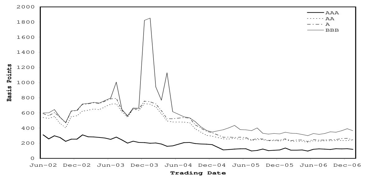
Notes: The portfolio comprises 150 bonds. \text{Notes: The portfolio comprises 150 bonds.} Notes: The portfolio comprises 150 bonds. Recoveries for each bond are assumed to be \text{Recoveries for each bond are assumed to be} Recoveries for each bond are assumed to be beta-distributed with a volatility of 0.25. \text{beta-distributed with a volatility of 0.25.} beta-distributed with a volatility of 0.25. Table 13: Portfolio Composition \text{Table 13: Portfolio Composition} Table 13: Portfolio Composition Portfolio Portfolio \text{Portfolio} \qquad \text{Portfolio} Portfolio Portfolio BB+ 0.080 0.076 \text{BB+} \qquad 0.080 \qquad 0.076 BB+ 0.080 0.076 Notes: The total value of the portfolio \text{Notes: The total value of the portfolio} Notes: The total value of the portfolio is Euro 238,035. \text{is Euro 238,035.} is Euro 238,035. Figure 6: Forward Default Probabilities for Investment Grade 2-Year Corporate \text{Figure 6: Forward Default Probabilities for Investment Grade 2-Year Corporate} Figure 6: Forward Default Probabilities for Investment Grade 2-Year Corporate AAA AA A BBB
Figure 7: Forward Default Probabilities for Investment Grade 5-Year Corporate \text{Figure 7: Forward Default Probabilities for Investment Grade 5-Year Corporate} Figure 7: Forward Default Probabilities for Investment Grade 5-Year Corporate BBB BB 4000 B CCC
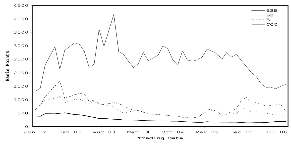
Figure 8: Forward Default Probabilities for Sub-Investment Grade 2-Year Cor- \text{Figure 8: Forward Default Probabilities for Sub-Investment Grade 2-Year Cor-} Figure 8: Forward Default Probabilities for Sub-Investment Grade 2-Year Cor- BBB BB B CCC
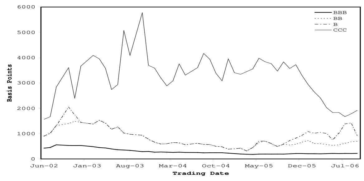
Figure 9: Forward Default Probabilities for Sub-Investment Grade 5-Year Cor- \text{Figure 9: Forward Default Probabilities for Sub-Investment Grade 5-Year Cor-} Figure 9: Forward Default Probabilities for Sub-Investment Grade 5-Year Cor- AAA AA 1800 A BBB
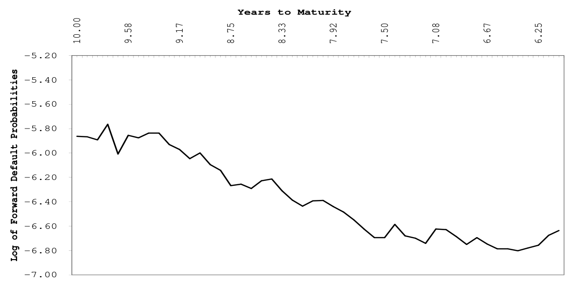
Figure 10: Forward Default Probabilities for 2-Year Maturity ABS (Recovery \text{Figure 10: Forward Default Probabilities for 2-Year Maturity ABS (Recovery} Figure 10: Forward Default Probabilities for 2-Year Maturity ABS (Recovery Years to Maturity 10.00 9.58 9.17 8.75 8.33 7.92 7.50 7.08 6.67 6.25 -5.20
-6.80 Log of Forward Default Probabilities
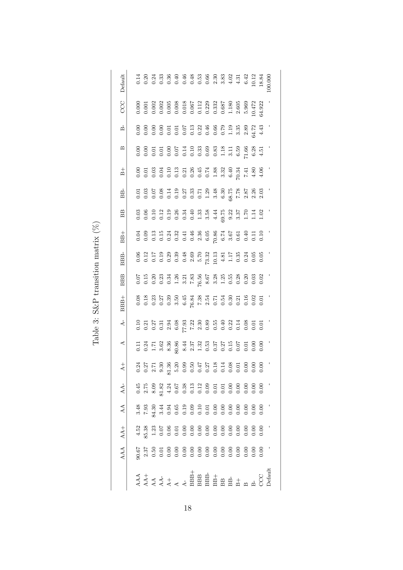
Figure 11: Constant-Calendar-Date Forward Default Probabilities for AAA Cor- \text{Figure 11: Constant-Calendar-Date Forward Default Probabilities for AAA Cor-} Figure 11: Constant-Calendar-Date Forward Default Probabilities for AAA Cor- Table 3 Copy link
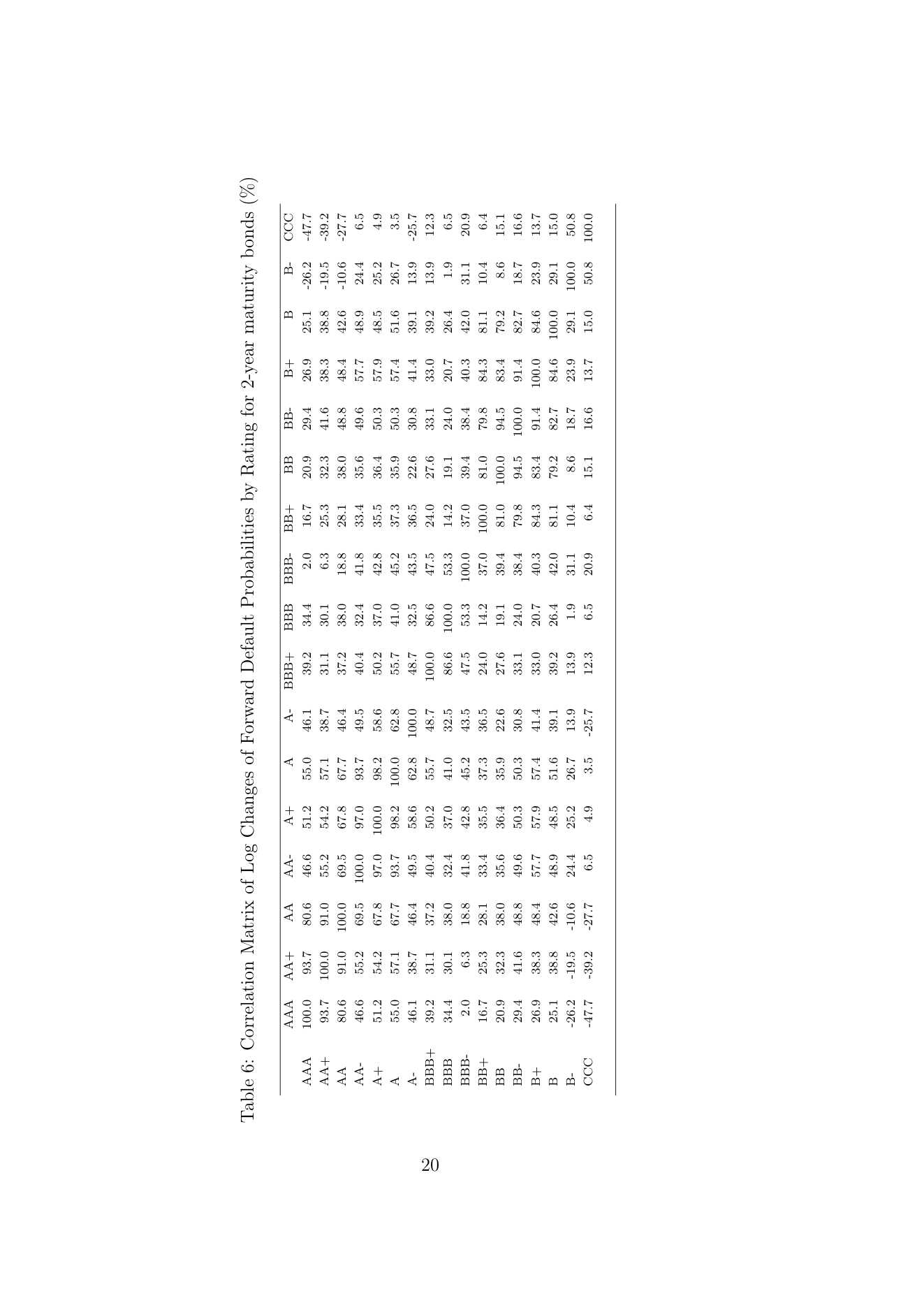
S&P transition matrix (%) Table 6 Copy link
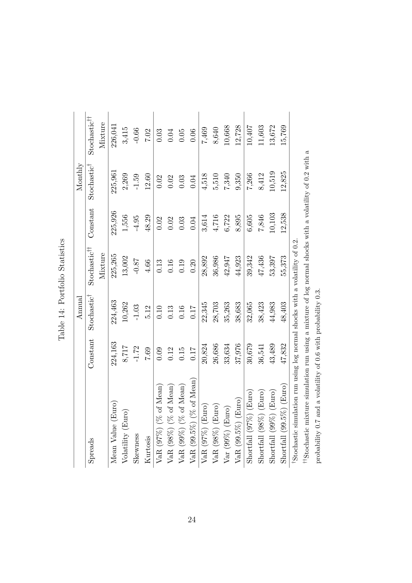
Correlation Matrix of Log Changes of Forward Default Probabilities by Rating for 2-year maturity bonds (%) Table 14 Copy link
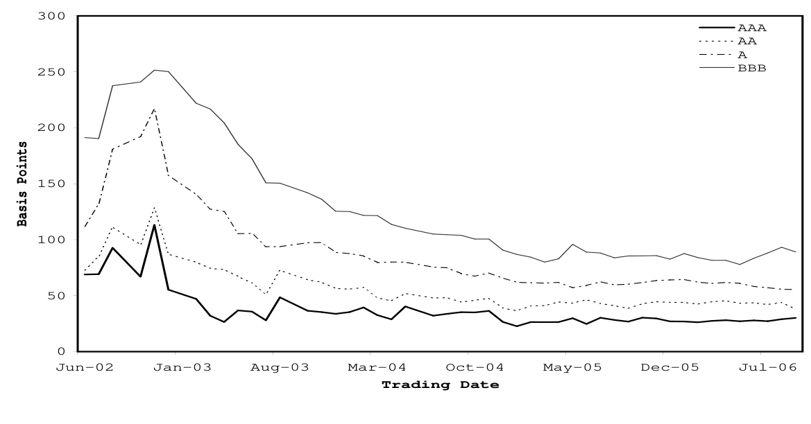
Portfolio Statistics Figure 1 Copy link
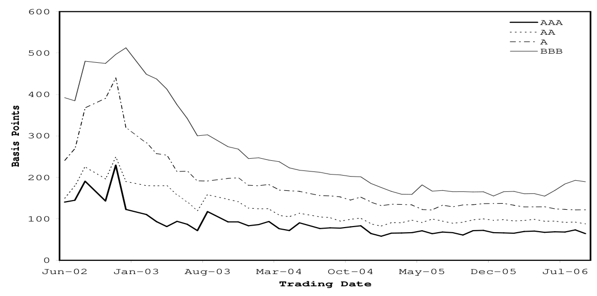
Investment Grade 2-Year Maturity Corporate Bond Spreads Figure 3 Copy link
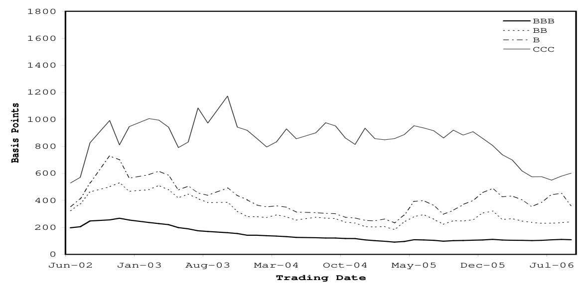
Sub-Investment Grade 2-Year Maturity Corporate Bond Spreads Figure 4 Copy link
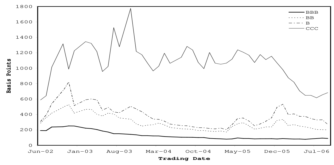
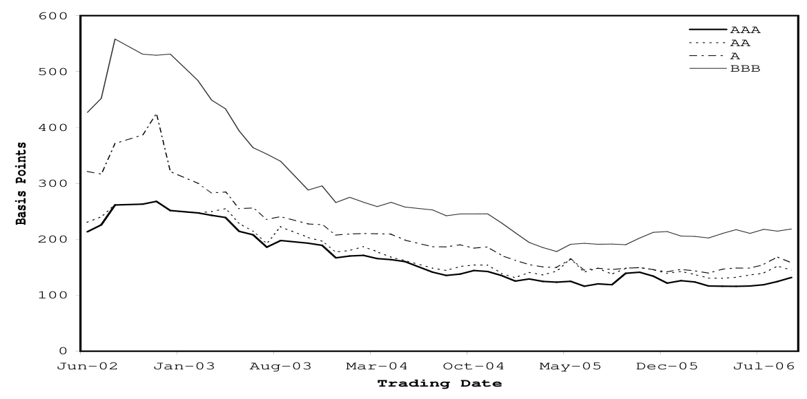
Sub-Investment Grade 5-Year Maturity Corporate Bond Spreads Figure 6 Copy link
Forward Default Probabilities for Investment Grade 2-Year Corporate Bonds Figure 7 Copy link
Forward Default Probabilities for Investment Grade 5-Year Corporate Bonds Figure 8 Copy link
Forward Default Probabilities for Sub-Investment Grade 2-Year Cor- porate Bonds Figure 9 Copy link
Forward Default Probabilities for Sub-Investment Grade 5-Year Cor- porate Bonds Figure 10 Copy link
Forward Default Probabilities for 2-Year Maturity ABS (Recovery 70%) Figure 11 Copy link
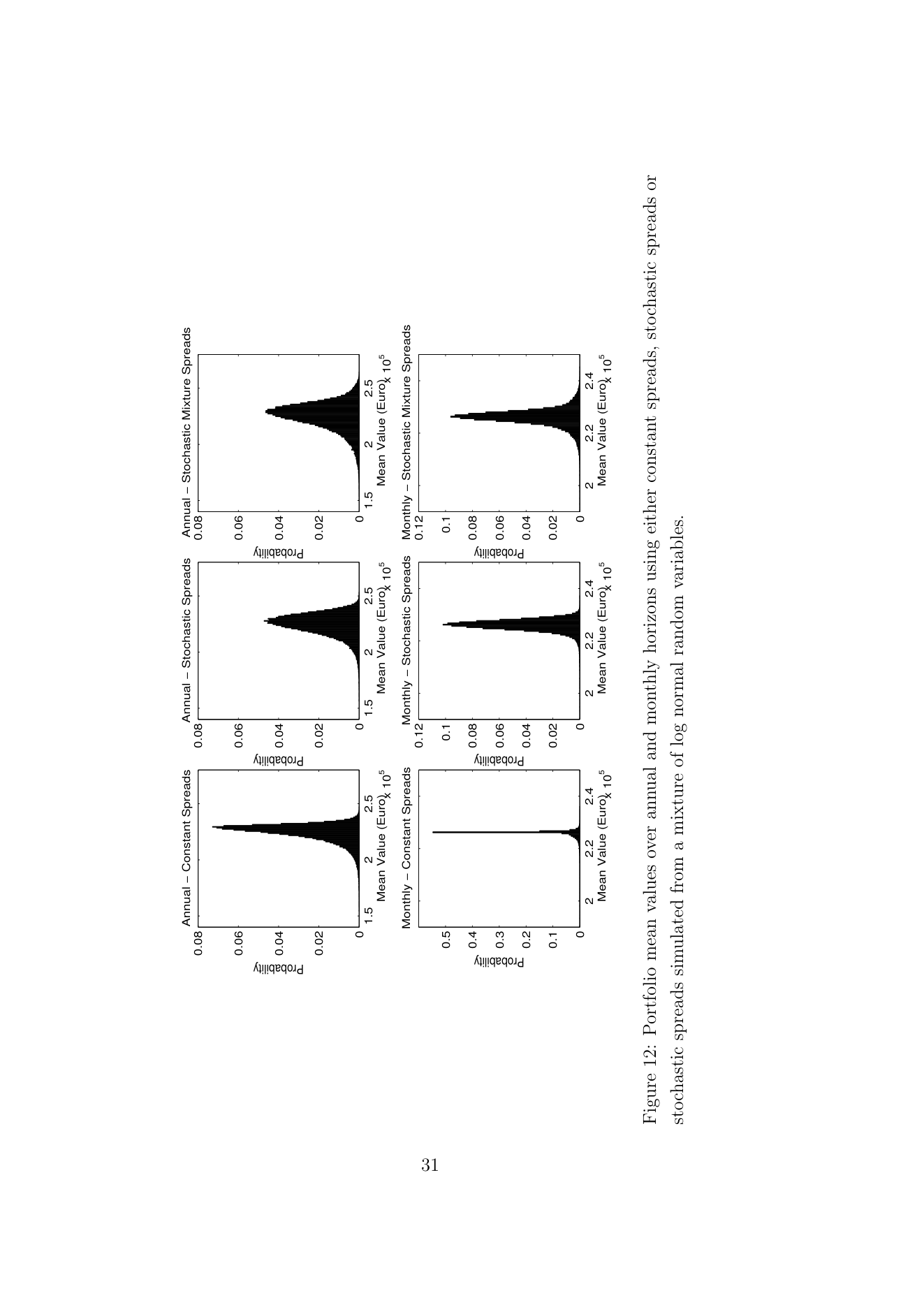
Constant-Calendar-Date Forward Default Probabilities for AAA Cor- porate Bonds Figure 12 Copy link
Portfolio mean values over annual and monthly horizons using either constant spreads, stochastic spreads or