

This note shows through a case study how Risk Control’s Stress ControllerTM software may be used to implement top down stress testing of a bank. The calculations are based on the publicly available financial statement and Pillar 3 disclosures of a large UK bank.
Top Down Stress Testing for Bank Financial Statements: A Case Study
Date: 19-11-2012 Number:12-62c
Executive Summary
This note shows through a case study how Risk Control’s Stress ControllerTM software may be used to implement top down stress testing of a bank. The calculations are based on the publicly available financial statement and Pillar 3 disclosures of a large UK bank.
We show how the balance sheet, P&L and key financial ratios are affected by scenarios involving recessions in America, Europe and the UK. A set of equations is constructed to describe the evolution of the bank’s financial statements.
Changes in the credit quality of the bank’s loan book and fluctuations in the value of mark-tomarket exposures affect asset values and income through provisions and mark-to-market asset write-offs. For a base case and for each of the stress scenarios, predictions are supplied for the bank’s key variables.
The results show how the bank’s impairment provisions rise, and capital, asset growth, returns on equity and profitability are depressed by the different recession scenarios. A UK-based recession has a larger impact than the other recession scenarios but shows a more rapid recovery.
Note that the framework used here may be used either with coarse, public data to perform top down stress testing or with highly granular internal bank data for bottom-up stress testing purposes. The financial statement modeling is highly flexible since equations may be written first in Excel, converted into scripts and then imported into the software for use at run-time to perform calculations.
For more information, contact: sales_enquiries@riskcontrollimited.com
Introduction
This note presents the results of an illustrative set of forecasts for the balance sheet of a major bank conditional on several macroeconomic scenarios.
The calculations are performed using Risk Control’s software Stress ControllerTM. This software permits the user to formulate a macroeconomic scenario and then to forecast conditional time paths for a wider set of macroeconomic variables for different geographical regions. The impact of the macroeconomic variable time paths on a bank’s portfolio may then be calculated and estimates of provisions may be fed into a model of the bank’s financial statements.
As an example bank, we have chosen Barclays Group PLC (hereafter referred to as the bank). The calculations presented here are based entirely on publicly disclosed data and have not been sanctioned or endorsed in any way by the bank. This bank has been selected as the example used in our case study because of its importance as a major UK bank with a strong international presence.
Using publicly available information from the bank’s annual report and Pillar 3 risk disclosures, we have:
1. Prepared appropriate historical macro data for the geographical regions within which the bank operates (i.e. Europe, UK, the Americas, Africa and the Middle East and Asia),
2. Extractedinformation from the bank’s annual report on its historical financial statements,
3. Generateda set of user-defined financial statements modeling equations.
4. Performed stressed financial forecasting calculations under different scenarios.
The scenarios we analyze are a base case and three stress scenarios. The three stress scenarios consist of 3-year recessions in (i) Europe, (ii) UK and (iii) the Americas respectively. In each case, the recession is specified to be negative shocks to real GDP of 2% and 1% in the first 2 quarters and of 0.5% in the subsequent 10 quarters.
The results are intuitive and convincing with capital ratios and indicators of profitability in the stress scenario cases following paths markedly below the baseline paths and with impairment provisions boosted and loan and deposit growth depressed compared to the base case.
Two important advantages of the software are as follows. First, the calculations presented here illustrate how one may use Stress ControllerTM to analyze bank financial statements and the vulnerability a bank exhibits with respect to macroeconomic shocks of different types even with relatively simple public data. Stress ControllerTM may also be used with complex and elaborate bank exposure data (for example, with tens or hundreds of thousands of underlying individual or semi-aggregated exposures) to perform bottom up stress analyses.
Second, the financial statement model employed consists of a set of equations linking balance sheet and P&L quantities (i) to macroeconomic variables, (ii) to provisions and mark-to-market write-offs based on exposures representing the bank’s assets, (iii) to user supplied parameters and variables (for example, capital injections and dividend payout rates). These equations may be created by the user of Stress ControllerTM and then imported as part of the data employed. At runtime, the software uses them to perform calculations. This approach ensures maximum flexibility.
1. Generating Consistent Macroeconomic Scenarios
In devising stress tests, one must first accomplish the (often challenging) task of generating consistent time paths for multiple macroeconomic variables. For example, one may wish to consider the impact of a recession in the US affecting say US GDP. However, this raises the issue of what is the impact on European or Asian GDP and also what happens to interest rates, exchange rates, inflation and commodity prices?
Risk Control’s Stress ControllerTM software contains an embedded macroeconomic model in which one may specify a series of shocks to a particular variable and calculate conditional forecasts of this and other variables into the future. The macroeconomic model employed is a statistical model commonly referred to as a Global Vector Autoregressive or GVAR model. Such models have been extensively used by academics and practitioners in economic forecasting units in central banks and other bodies to forecast macro time series.
It is important to allow for contagion between regions in the propagation of macroeconomic scenarios.GVAR models suppose that for each geographical region there exists a vector of macroeconomic variables which evolve linearly over time as non-stationary but cointegrated time series. The variables in each region are affected by their own lagged values and by weighted sums of variables from other regions.
The GVAR model included in Stress ControllerTM is highly flexible in that one may readily change the countries and regions. In the exercise reported in this note, we adopt a set of regions consistent with the bank’s approach to categorizing its loan exposures. Specifically, we suppose that the regions comprise: (a) UK, (b) Europe (excluding the UK), (c) the Americas (comprising South, Central and North American countries), (d) the Middle East and Africa, and (e) Asia.
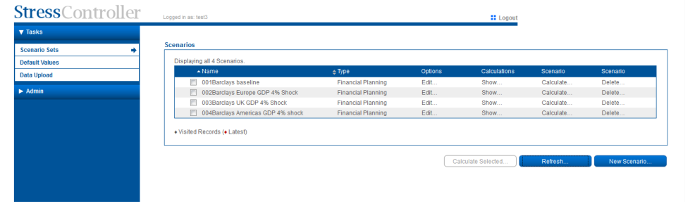
To set up scenarios within Stress ControllerTM, one operates through the web-based interface. Scenarios are stored within an underlying relational database and repeated calculations may be performed for a given scenario after amendments are made to the scenario itself or after the underlying data has been updated. Figure 1 shows the list of scenarios within the Stress ControllerTM web-based interface.
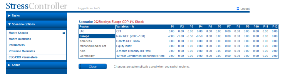
Figure 2 shows a screen shot during the editing of a scenario. Scenarios consist of sequences of period-by-period shocks to macroeconomic variables. Non-interest-rate macro time series are stored in log form. Hence, a shock of negative one unit in a given quarter to a scenario variable such as GDP corresponds to a minus 1% innovation.
Stress ControllerTM produces time paths of macroeconomic variables such as those shown in
Figure 3. These time series are the mean values of the variables in question conditional on the
one may import a scenario in the form of a set of time series for different macroeconomic variables. Hence, one may work with scenarios generated by regulators or a bank economicsdepartment, importing the scenario time series into the application and then performing additional calculations with them.
Figure 3: Results on GDP time paths for different regions
2. The Bank’s Loan Portfolio
Loan Data
This section presents a description of the bank’s loan books based on its Pillar 3 disclosures as recorded in its annual report. The bank provides information on the breakdown of its loan book by region, sector, credit quality, and asset class. Table 1 shows the matrix of sector and region loan volumes. These figures are taken directly from the bank’s 2011report except for small changes. (For example, the division between wholesale to customer and wholesale to bank for the Government and central bank category is based on other data disclosed by the bank.)
Table 2 shows the distribution by credit quality. The figures here reflect our assumption that the breakdown by credit quality of Wholesale to bank, Wholesale to customer and Other retail are the same. Table 3 contains information about the probability of default (PD) for different asset classes and credit quality groups. These figures are chosen to be representative numbers within PD ranges provided for each category by the bank. The bank provides information on both PDs and loss rates. Using these, we infer the recovery rates specified in the right hand column.
230,436 105,148 77,094 52,543 14,159 479,380 Source: the table ‘Loans by region and sector’ on page 93 of the bank’s Annual Report 2011.
In Table 4, we confirm that the calibrated loss rates approximately match the reported loss rates quoted by the bank. To achieve this we adjust the PD and recovery rates in Table 3 to ensure that, for each asset class, the loss given default rate from our model (displayed in second column of Table 4) matches the target loss rate disclosed by the bank (displayed in the third column of Table 4).
Loan Modeling and Sensitivities
One may model loans within Stress ControllerTM either as individual rated exposures or as diversified pool exposures with a default rate that evolves over time. For public data analysis such as the exercise reported in this paper, we use diversified pool exposures.
In separate publications, we have shown how to derive simple but rigorous models of the dynamic behavior of loss rates on pools of homogeneous loans. These may be modeled unconditionally or conditional on macroeconomic variables. In the latter case, the default rate evolves as an auto-correlated time series driven by shocks to macro variables like GDP, interest rates or unemployment.
The sensitivities we employ in this case study are sector-specificand asset-class-specific and draw on the estimates we have obtained in a series of past studies of the macroeconomic impact on loan books using data from different banks and a range of public data sources.
| Africa | and | |||||||||
|---|---|---|---|---|---|---|---|---|---|---|
| Middle | ||||||||||
| Industrial sectors | credit | class | UK | Europe | Americas | East | Asia | Total | ||
| Banks | Wholesale | to | bank | 9,251 | 13,503 | 13,349 | 2,956 | 5,648 | 44,707 | |
| Other financial | institutionsa | Wholesale | to | customer | 18,474 | 20,059 | 44,965 | 2,264 | 3,888 | 89,650 |
| Manufacturing | Wholesale | to | customer | 6,185 | 3,341 | 1,396 | 1,439 | 543 | 12,904 | |
| Construction | Wholesale | to | customer | 3,391 | 771 | 32 | 348 | 65 | 4,607 | |
| Property | Wholesale | to | customer | 16,230 | 3,193 | 869 | 3,600 | 212 | 24,104 | |
| Government and | central bank | Wholesale | to | customer | 341 | 2,326 | 627 | 2,123 | 713 | 6,129 |
| Government and | central bank | Wholesale | to | bank | 152 | 1,039 | 280 | 949 | 318 | 2,739 |
| Energy and water | Wholesale | to | customer | 1,599 | 2,448 | 2,165 | 818 | 384 | 7,414 | |
| Wholesale and | retail distribution and leisure | Wholesale | to | customer | 10,308 | 3,008 | 656 | 2,073 | 161 | 16,206 |
| Business and other | services | Wholesale | to | customer | 16,473 | 4,981 | 1,584 | 2,907 | 355 | 26,300 |
| Home loans | Home loans | 112,260 | 38,508 | 566 | 19,437 | 501 | 171,272 | |||
| Cards, unsecured | loans and other personal lending | Cards | 27,409 | 6,417 | 9,293 | 6,158 | 785 | 50,062 | ||
| Other wholesale | Wholesale | to | customer | 3,181 | 2,112 | 499 | 2,841 | 223 | 8,856 | |
| Other retail | Other retail | 5,182 | 3,442 | 813 | 4,630 | 363 | 14,430 |
| Performing | Performing | Performing Past | due not | Impaired Impaired | |||
|---|---|---|---|---|---|---|---|
| Asset classes strong | satisfactory | higher | risk | impaired | collectively individually | Total | |
| Wholesale to bank | 0.6516 | 0.2490 | 0.0193 | 0.0382 | 0.0033 | 0.0386 | 1 |
| Wholesale to customer | 0.6516 | 0.2490 | 0.0193 | 0.0382 | 0.0033 | 0.0386 | 1 |
| Home loans | 0.7786 | 0.1502 | 0.0063 | 0.0007 | 0.0620 | 0.0022 | 1 |
| Cards | 0.2061 | 0.6575 | 0.0150 | 0.0050 | 0.1062 | 0.0102 | 1 |
| Other retail | 0.6516 | 0.2490 | 0.0193 | 0.0382 | 0.0033 | 0.0386 | 1 |
Source: the table ‘Credit quality of L&A’ on page 104 of the bank’s Annual Report 2011.
| Performing | Performing | Performing | Past due | not Impaired | Impaired | recovery | |
|---|---|---|---|---|---|---|---|
| Asset classes strong | satisfactory | higher | risk impaired | collectively | individually | ratio | |
| Wholesale to bank | 0.01 | 0.02 | 0.03 | 15 | 20 | 20 | 0.99 |
| Wholesale to customer | 0.01 | 0.6 | 11 | 15 | 20 | 20 | 0.6 |
| Home loans | 0.3 | 2 | 10 | 15 | 20 | 20 | 0.7 |
| Cards | 0.6 | 5 | 12 | 15 | 20 | 20 | 0.5 |
| Other retail | 0.4 | 2 | 10 | 15 | 20 | 20 | 0.55 |
Source: the table ‘Internal measures of credit quality’ on page 105 of the bank’s Annual Report 2011.
| calibrated | ||||
|---|---|---|---|---|
| weighted | ||||
| amount | weight | average | LGD target | loss |
| Asset classes of each | class | (bps) rate | (bps) | |
| Wholesale to bank | 0.099 | 1.423 | 1.265 | |
| Wholesale to customer | 0.409 | 71.176 | 69.430 | |
| Home loans | 0.357 | 56.750 | 50.000 | |
| Cards | 0.104 | 299.733 | 300.000 | |
| Other retail | 0.030 | 106.326 | 102.730 |
3. Modeling Financial Statements
The Bank’s Financial Statements
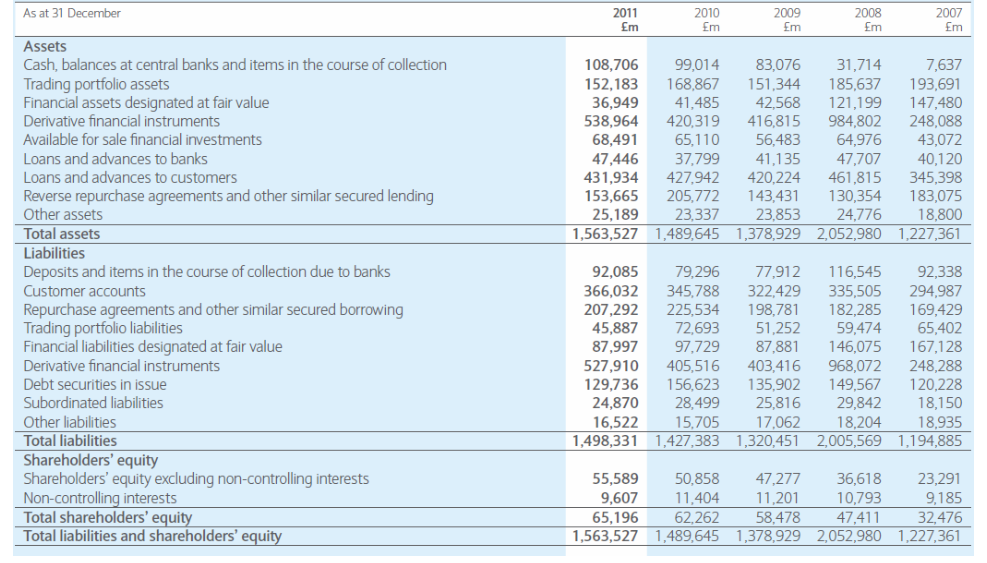
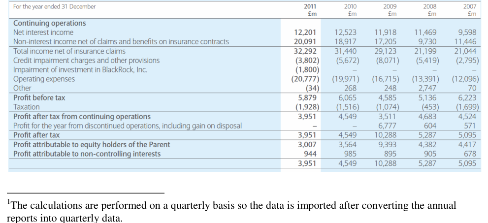
In Figures 4 and 5, the historical consolidated summary financial statements of the bank are presented for the past 5 years. These historical financial statements are imported into Stress ControllerTM and serve as the starting point for forecasts of future financial statements conditional on macroeconomic scenarios.[1]
Modeling the Bank’s Balance Sheet
Detailed description of the equations used in modeling the bank’s balance sheet and P&L are provided in the Appendix. Key assumptions of the modeling approach are as follows.
1. We view the bank’s financial statement as balance-sheet driven. Both sides of the balance sheet are assumed to be directly affected by the macro-economy. The asset side is also affected through the impact of macro shocks on provisions and changes in mark-tomarket values.
2. Loans and deposits are assumed to be linked to (a) GDP growth in the relevant region, and (b) its own historical trend. The relative importance of (a) and (b) and the sensitivity to macro shocks vary for different loans and deposits. The approach employed in this case study could easily be generalized to include interest rates or other macroeconomic variables such as unemployment rates but we have preferred in this exercise to keep the analysis as simple as possible.
3. Marked-to-market assets and liabilities are assumed to be sensitive to relevant macro indicators, in particular to GDP or national equity indices.
4. Items such as ‘Cash’ and ‘Others Assets/Liabilities/Expenses’ are modeled as moving averages of the previous balances.
5. All Balance Sheet items, except ‘Cash’ and ‘Other Assets/Liabilities’, have been modeled taking into account inflation.
6. Income is modeled based on the forecasted balance-sheet. Both interest and non-interest income are modeled as being affected by the combined changes in loan-type assets and non-loan type assets, but with different weights on different types of assets (e.g. weight of loan-type assets on interest income is 0.8 but on non-interest income is 0.2) and the weights are user-defined parameters. For interest income, the impact from changes of forecasted interest rates is modeled
7. The credit impairment charge is calculated as the expected losses of loans and advances to retail and wholesale customers, taking into account the lagged impact of macroeconomic variables on provisions. (Recall that loans are modeled as diversified pool exposures.)
8. We view the operating expenses of the bank as controlled by the management rather than reacting passively to changes in the size of the bank’s balance-sheet. We therefore allow the user to input the forecasted rate of change of operating expenses.
9. To balance the balance sheet at the end of each forecasting, we adjust the gap between forecast ‘Total Assets’ and ‘Total Liabilities and Shareholder Equities’, allowing this gap to be absorbed by multiple items employing user-defined weights. The items adjusted to balance assets and liabilities are referred to as the B/S ‘balancing items’.
10. We model shareholders’ equity changes as influenced by: (i) retained earnings from the forecast Income Statements, (ii) dividend payouts based on user defined ‘dividend payout ratios’ and (iii) reserve and employee share scheme changes which are also user-defined.
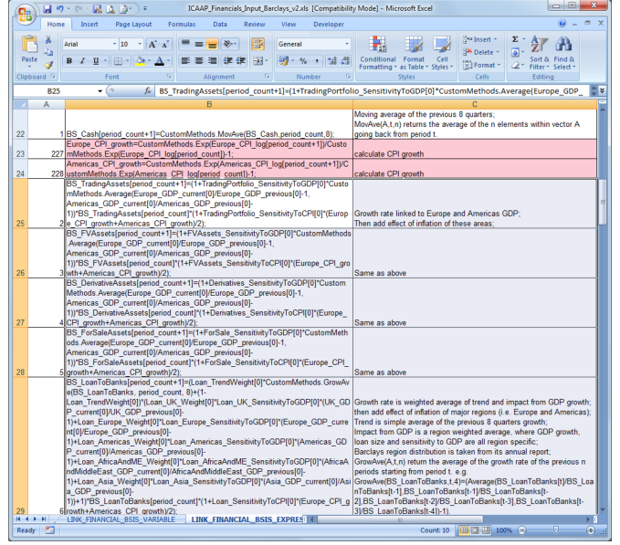
The equations for the financial statements analysis are treated in Stress ControllerTMas part of the data of the model. They are imported from a ‘feeder’ Excel workbook. A screenshot of the equations stored in such a workbook is provided in Figure 6.
To take an example, the item ‘Trading portfolio assets’ is modeled as: BS_TradingAssets[period_count+1]=(1+TradingPortfolio_SensitivityToGDP[0]*Custom Methods.Average(Europe_GDP_current[0]/Europe_GDP_previous[0]-1, Americas_GDP_current[0]/Americas_GDP_previous[0]- 1))*BS_TradingAssets[period_count]*(1+TradingPortfolio_SensitivityToCPI[0]*(Europ e_CPI_growth+Americas_CPI_growth)/2);
Figure 7:ForecastedGDPyear-on-year growth under 4 scenarios
Europe Recession Base Case
Americas Recession UK Recession
Note: In Figure 1 we plot out, in each scenario, the historical year-on-year GDP growth for the past 8 quarters and the forecasted year-on-year GDP growth for the future 12 quarters.
Before the above equation is executed, all the variables employed in the equation must be declared by importing a user workbook containing the definition of each variable. Further details of how the equations are specified and used within Stress ControllerTM are provided in the Appendix.
4. Results
Using the approach described above, we performed an analysis of the impact of several stress scenarios on the bank’s financial statements and key risk indicators. We present below results for
(i) a base case (i.e., an unconditional forecast), (ii) a European recession, (iii) a UK recession, and (iv) a recession in America.
Figure 7 shows the time paths of real GDP 1-year growth rates for the UK, Europe and America. The time paths are shown for the base case and the three stress cases described above. We display quarterly data up to the end of 2011 followed by projections quarter by quarter until the end of
2014. Note that we start the forecast calculations in Q1 2012 because the financial statement data available is for the end of 2011.
The recession scenarios assume a sequence of shocks to real GDP in the geographical region in question. In all cases, the shocks are -2% in Q1, -1% in Q2 and -0.5% in Q3, Q4,.., Q12. These shocks sum to a cumulative negative shocks of 8% over 3 years.
As one might expect, the impact of a recession is greatest for the region itself. However, recessions in each region have serious implications for outcomes in other regions. Note that the fact that American and European GDP growth rates are affected by a UK recession does not imply a direct causal relationship. Instead, the implication is that when a recession occurs in the UK, on average one would expect recessions of the magnitude shown in the other regions.
Figure 8 shows the path of credit impairment provisions under the four scenarios considered. The impairments are driven by the impact of GDP shocks on the expected losses of the diversified pool exposures included in the software to describe the bank’s loan book. These are broken down by sector, credit quality and geographical region.
As one may observe from Figure 8, impairment provisions are slightly downward sloping in the base case but rise significantly in the three recession scenarios, showing particular ly striking growth in the UK recession scenario. In this latter scenario, one may note that provisions start to decline towards the end of the period, reflecting the bounce back in growth that occurs in the UK when the recession is primarily a UK phenomenon (see Figure 7).
Figure 9 presents a series of plots of key financial indicators under the four scenarios. Capital, measured in different ways, is down in all three recession scenarios. Capital recovers towards the baseline path in the UK recession scenario by the end of the period but remains stubbornly low in the Europe and Americas recession scenarios.
The figures for returns on equity and Risk Weighted Assets shown in Figure 9 again show consistent patterns of decline as the recessions emerge. In the case of the UK recession scenario, returns recover towards baseline levels towards the end of the period under consideration.
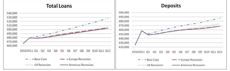
Tables 5 and 6 and Figures 10 and 11 show selected items from the bank’s balance sheet and income statements. Loan and deposit growth are depressed in the recession scenarios. Total income and profits are down, the latter being hit most badly in the UK recession scenario but then recovering relatively quickly in this case.
Figure 11: Extracted items from forecasted quarterly income statements (£m)
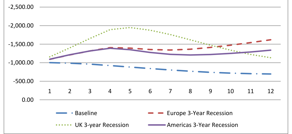
Note: based on the credit risk modeling of a static credit portfolio, we have also taken into account (a) the variation of the loans over the forecasted period and (b) the lag effect of GDP shock to the provision of credit loans.
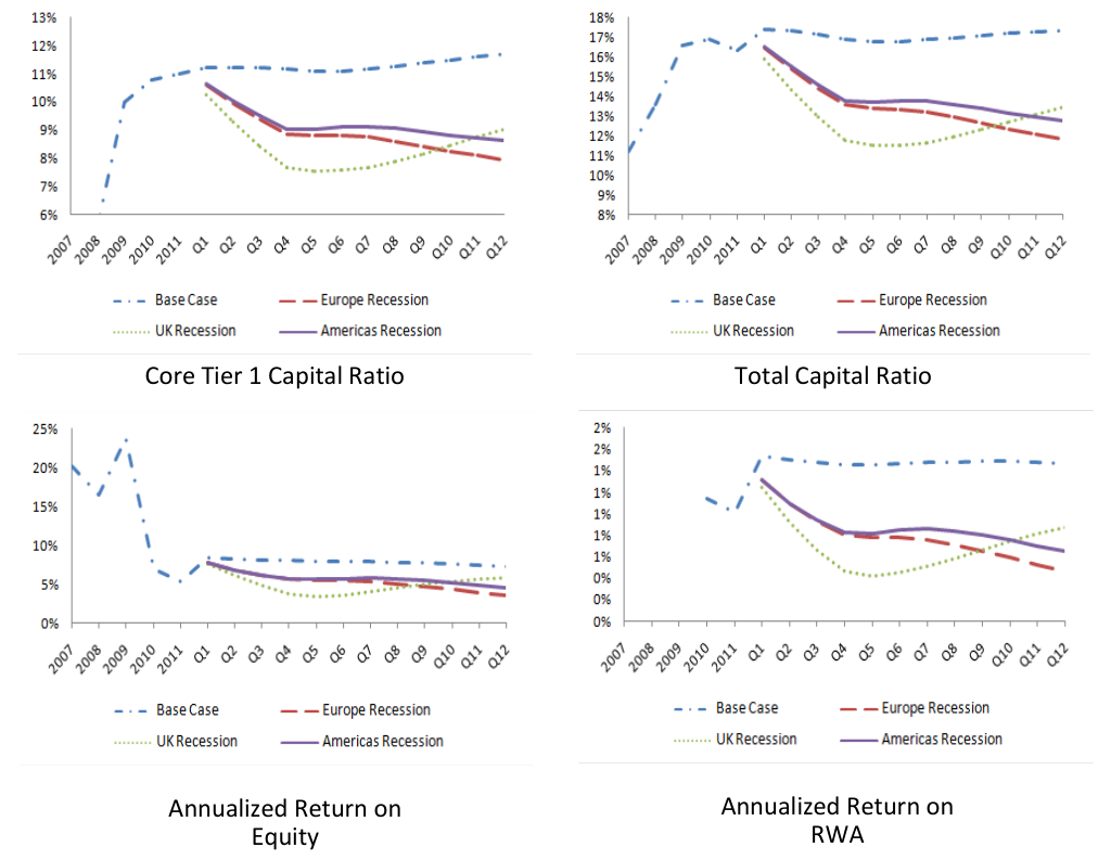
Note: We plot out the KPI measure for the previous 5 years and future 12 forecasted quarters.
| Base | Case | 2010 | 2011 | Q1 | Q2 | Q3 | Q4 | Q5 | Q6 | Q7 | Q8 | Q9 | Q10 | Q11 | Q12 |
|---|---|---|---|---|---|---|---|---|---|---|---|---|---|---|---|
| Cash and | Mark-to-Market Assets | 794,795 | 905,293 | 901,894 | 907,980 | 914,382 | 920,548 | 926,410 | 932,096 | 937,563 | 942,768 | 947,664 | 953,655 | 959,594 | 965,447 |
| Total Loans | 465,741 | 479,380 | 482,535 | 485,911 | 489,488 | 493,243 | 497,160 | 501,214 | 505,381 | 509,642 | 513,982 | 518,383 | 522,833 | 527,321 | |
| Other Assets | 229,109 | 178,854 | 202,718 | 204,878 | 205,730 | 204,747 | 201,700 | 199,846 | 199,333 | 200,332 | 203,031 | 203,075 | 202,852 | 202,494 | |
| Total Assets | 1,489,645 | 1,563,527 | 1,587,148 | 1,598,769 | 1,609,600 | 1,618,538 | 1,625,270 | 1,633,155 | 1,642,277 | 1,652,742 | 1,664,677 | 1,675,113 | 1,685,279 | 1,695,261 | |
| Deposits | 425,084 | 458,117 | 451,050 | 454,604 | 458,673 | 462,526 | 465,923 | 469,050 | 471,938 | 474,577 | 476,931 | 480,471 | 483,984 | 487,406 | |
| Mark-to-Market | Liabilities | 801,472 | 869,086 | 881,228 | 886,616 | 891,438 | 895,583 | 898,938 | 902,792 | 907,190 | 912,187 | 917,848 | 922,650 | 927,345 | 932,000 |
| Other Liabilities | 200,827 | 171,128 | 187,936 | 188,869 | 189,042 | 188,185 | 186,340 | 185,382 | 185,318 | 186,215 | 188,173 | 188,283 | 188,242 | 188,137 | |
| Total Liabilities | 1,427,383 | 1,498,331 | 1,520,214 | 1,530,088 | 1,539,152 | 1,546,295 | 1,551,201 | 1,557,223 | 1,564,446 | 1,572,978 | 1,582,951 | 1,591,404 | 1,599,572 | 1,607,544 | |
| Total Equity | 62,262 | 65,196 | 66,934 | 68,681 | 70,448 | 72,243 | 74,069 | 75,932 | 77,831 | 79,764 | 81,726 | 83,709 | 85,707 | 87,717 | |
| Total Liabilities | and Equity | 1,489,645 | 1,563,527 | 1,587,148 | 1,598,769 | 1,609,600 | 1,618,538 | 1,625,270 | 1,633,155 | 1,642,277 | 1,652,742 | 1,664,677 | 1,675,113 | 1,685,279 | 1,695,261 |
| UK | Recession | 2010 | 2011 | Q1 | Q2 | Q3 | Q4 | Q5 | Q6 | Q7 | Q8 | Q9 | Q10 | Q11 | Q12 |
| Cash and | Mark-to-Market Assets | 794,795 | 905,293 | 898,512 | 902,084 | 906,901 | 911,864 | 916,580 | 921,152 | 925,517 | 929,620 | 933,405 | 938,179 | 942,911 | 947,562 |
| Total Loans | 465,741 | 479,380 | 478,178 | 479,167 | 481,288 | 483,448 | 485,659 | 488,054 | 490,682 | 493,538 | 496,603 | 499,855 | 503,266 | 506,704 | |
| Other Assets | 229,109 | 178,854 | 202,855 | 204,917 | 205,643 | 204,648 | 201,586 | 199,713 | 199,180 | 200,153 | 202,824 | 202,820 | 202,557 | 202,171 | |
| Total Assets | 1,489,645 | 1,563,527 | 1,579,545 | 1,586,169 | 1,593,832 | 1,599,959 | 1,603,825 | 1,608,919 | 1,615,379 | 1,623,311 | 1,632,832 | 1,640,855 | 1,648,734 | 1,656,437 | |
| Deposits | 425,084 | 458,117 | 448,628 | 449,990 | 452,585 | 455,418 | 457,882 | 460,149 | 462,259 | 464,191 | 465,905 | 468,731 | 471,567 | 474,287 | |
| Mark-to-Market | Liabilities | 801,472 | 869,086 | 876,543 | 879,859 | 883,662 | 886,773 | 889,134 | 892,013 | 895,438 | 899,453 | 904,114 | 907,946 | 911,634 | 915,252 |
| Other Liabilities | 200,827 | 171,128 | 187,605 | 188,188 | 188,294 | 187,510 | 185,637 | 184,621 | 184,492 | 185,315 | 187,192 | 187,187 | 187,089 | 186,939 | |
| Total Liabilities | 1,427,383 | 1,498,331 | 1,512,776 | 1,518,036 | 1,524,541 | 1,529,701 | 1,532,654 | 1,536,783 | 1,542,189 | 1,548,960 | 1,557,210 | 1,563,864 | 1,570,291 | 1,576,478 | |
| Total Equity | 62,262 | 65,196 | 66,769 | 68,133 | 69,292 | 70,258 | 71,171 | 72,137 | 73,191 | 74,351 | 75,622 | 76,990 | 78,443 | 79,959 | |
| Total Liabilities | and Equity | 1,489,645 | 1,563,527 | 1,579,545 | 1,586,169 | 1,593,832 | 1,599,959 | 1,603,825 | 1,608,919 | 1,615,379 | 1,623,311 | 1,632,832 | 1,640,855 | 1,648,734 | 1,656,437 |
| Total | Income | 31,440 | 32,292 | 8,126 | 8,181 | 8,238 | 8,297 | 8,357 | 8,419 | 8,481 | 8,544 | 8,607 | 8,671 | 8,735 | 8,799 |
|---|---|---|---|---|---|---|---|---|---|---|---|---|---|---|---|
| Credit | Impairment Charge | -5,672 | -3,802 | -1,003 | -988 | -962 | -923 | -883 | -843 | -804 | -770 | -741 | -719 | -704 | -695 |
| Total | Expenses | -19,703 | -22,611 | -5,217 | -5,274 | -5,332 | -5,392 | -5,453 | -5,505 | -5,558 | -5,612 | -5,665 | -5,724 | -5,783 | -5,841 |
| Profit | before Tax | 6,065 | 5,879 | 1,906 | 1,919 | 1,944 | 1,982 | 2,022 | 2,071 | 2,118 | 2,162 | 2,201 | 2,228 | 2,249 | 2,263 |
| Profit | after Tax | 4,549 | 3,951 | 1,525 | 1,535 | 1,555 | 1,586 | 1,617 | 1,656 | 1,695 | 1,730 | 1,761 | 1,783 | 1,799 | 1,810 |
| 2010 | 2011 | ||||||||||||||
| UK Recession | annual | annual | Q1 | Q2 | Q3 | Q4 | Q5 | Q6 | Q7 | Q8 | Q9 | Q10 | Q11 | Q12 | |
| Total | Income | 31,440 | 32,292 | 8,064 | 8,088 | 8,131 | 8,176 | 8,224 | 8,274 | 8,325 | 8,377 | 8,430 | 8,483 | 8,537 | 8,590 |
| Credit | Impairment Charge | -5,672 | -3,802 | -1,157 | -1,399 | -1,652 | -1,892 | -1,948 | -1,877 | -1,759 | -1,617 | -1,472 | -1,338 | -1,223 | -1,133 |
| Total | Expenses | -19,703 | -22,611 | -5,217 | -5,274 | -5,332 | -5,392 | -5,453 | -5,505 | -5,558 | -5,612 | -5,665 | -5,724 | -5,783 | -5,841 |
| Profit | before Tax | 6,065 | 5,879 | 1,690 | 1,415 | 1,147 | 893 | 824 | 892 | 1,008 | 1,149 | 1,293 | 1,421 | 1,531 | 1,615 |
| Profit | after Tax | 4,549 | 3,951 | 1,352 | 1,132 | 917 | 714 | 659 | 714 | 807 | 919 | 1,034 | 1,137 | 1,225 | 1,292 |
Contacts:
William Perraudin, Director Telephone: +44 20 3307 0731 (o), +44 7968 328 459 (m) Email: william.perraudin@riskcontrollimited.com
FrederikBurlage, Sales Telephone: +44 20 3307 0739 (o), +44 7834 542 020 (m) Email: frederik.burlage@riskcontrollimited.co.uk
Appendix
Section A.1: Introduction
This Appendix provides information on how one may write a financial statement model for a bank for use in Stress ControllerTM. We present an illustrative model fora particular bank, namely the Barclays Group PLC. TheAppendix is organized as follows.In section A.2, we give a specific example of how to declare all the variables that will be employed in an example equation. In section A.3, we explain how each balance sheet (B/S) item within the ‘Assets’ and ‘Liabilities’ categories are forecast. In section A.4, we illustrate the forecasting of the income statement (I/S) and in section A.5, the forecasting of B/S items within the ‘Shareholders’ equity’ category. Finally, in A.6, we show how one balance the B/S by recalculating the ‘balancing items’.
Section A.2: Variables Declaration
Before the equations of financial statements modeling can be executed, variables employed in the equations must be loaded into the database by importing a user workbook in which the definition of each variable is specified.
The definition of each variable is stored in a string consisting of four sections. Each section must adhere to certain rules. The four sections are:
(1) Major category:
(2) Name of the variable
(3) Minor category
(4) Indicators for database management
The sections are separated by hyphens. (Note that the hyphen symbol is therefore a reserved character that should not be used for other purposes.)
To illustrate the declaration of variables, consider the B/S variable: ‘Trading portfolio assets’. This is modeled as:
BS_TradingAssets[t+1]=(1+TradingPortfolio_SensitivityToGDP[0]* CustomMethods.Average(Europe_GDP[t+1]/Europe_GDP[t]-1, Americas_GDP[t+1]/Americas_GDP[t]- 1))*BS_TradingAssets[t]*(1+TradingPortfolio_SensitivityToCPI [0]*(Europe_CPI_growth+Americas_CPI_growth)/2);
For the above equation to be valid, the user must declare the variables it includes as follow:
(1) BS_TradingAssets Group-Trading portfolio assets-BS-1-1-3-0
• ‘Group’: this indicates the variable is group level data;
• ‘BS’: this indicates the variable is from the B/S;
• ‘Trading portfolio assets’: this is the name of the variable as it appears in the B/S;
• ‘1-1-3-0’: this code specifies that the variable (i) will be saved in the database, (ii) will be displayed in the interface, (iii) will have the relative position 3 in the interface and (iv) will not be highlighted.
The time series indicator [t+1] implies that this variable has a time dimension, and [t+1] represents the period to be calculated and [t] the first lag.
(2) TradingPortfolio_SensitivityToGDP Parameter-Group TradingPortfolio_SensitivityToGDP-SCALAR-1-1-1-0
‘Parameter’: this is a user-defined parameter that will be imported from a user-supplied workbook;
‘SCALAR’: this indicates the parameter is scalar valued (and has no time dimension);
‘Group TradingPortfolio’: this is the name of the parameter in the user-supplied workbook;
The time series indicator [0] implies that this variable has no time-series dimension.
(3) Europe_GDP Macro-Europe:Real GDP (2005=100)-MACRORESULT-1-1-1-0
‘Macro’: this indicates the variable is a variable supplied by the macro model;
‘MACRORESULT’: this item should be fetched from the macro results within Stress ControllerTM;
‘Europe:Real GDP (2005=100)’: this is the name of the macro variable;
The time series indicator [t+1] implies that this variable has time dimension, and [t+1] represents the period to be calculated and [t] its first lag.
Section A.3: B/S-Assets and Liabilities
In this section, we explain the modeling of each B/S item.
Assets
1. Cash, balance at central banks and items in the course of collection
This item is estimated as the average of the previous 8 quarters.Note that this item may be adjusted in the rebalancing of the balance sheet.
BS_Cash[t+1]=CustomMethods.MovAve(BS_Cash,t,8);
2. Trading portfolio assets
The growth rate of this item is estimated as being sensitive to the GDP growth rates of Europe and Americas, where sensitivity is a user-defined parameter. Modeling has taken into account inflation changes. Please note that this item might be recalculated for rebalancing the balance sheet.
3. BS_TradingAssets[period_count+1]=(1+TradingPortfolio_SensitivityToGDP[0]*Custom Methods.Average(Europe_GDP_current[0]/Europe_GDP_previous[0]-1, Americas_GDP_current[0]/Americas_GDP_previous[0]- 1))*BS_TradingAssets[period_count]*(1+TradingPortfolio_SensitivityToCPI[0]*(Europ e_CPI_growth+Americas_CPI_growth)/2);Financial assets designated at fair value
Same as above, while sensitivity set as a separate parameter. Modeling has taken into account the inflation changes.
BS_FVAssets[t+1]=(1+FVAssets_SensitivityToGDP[0]*CustomMethods.Average(Euro pe_GDP[t+1]/Europe_GDP[t]-1, Americas_GDP[t+1]/Americas_GDP[t]- 1))*BS_FVAssets[t] *(1+FVAssets_SensitivityToCPI[0]*(Europe_CPI_growth+Americas_CPI_growth)/2);
4. Derivative financial instruments assets
As above except that the sensitivity is set as a separate parameter. Modeling has taken into account inflation.
BS_DerivativeAssets[t+1]=(1+Derivatives_SensitivityToGDP[0]*CustomMethods.Avera ge(Europe_GDP[t+1]/Europe_GDP[t]-1, Americas_GDP[t+1]/Americas_GDP[t]- 1))*BS_DerivativeAssets[t] *(1+Derivatives_SensitivityToCPI[0]*(Europe_CPI_growth+Americas_CPI_growth)/2);
5. Available for sale financial investments
Same as above except that the sensitivity set as a separate parameter. Modeling has taken into account inflation.
BS_ForSaleAssets[t+1]=(1+ForSale_SensitivityToGDP[0]*CustomMethods.Average(Eu rope_GDP[t+1]/Europe_GDP[t]-1, Americas_GDP[t+1]/Americas_GDP[t]- 1))*BS_ForSaleAssets[t] *(1+ForSale_SensitivityToCPI[0]*(Europe_CPI_growth+Americas_CPI_growth)/2);
6. Gross loans and advances to banks
The growth rate of this item is estimated as the weighted average of (1) impact from trend and (2) GDP growth. The weights are user-defined parameters and impact from trend is calculated as the average growth rate of previous 8 quarters. The GDP growth is a regionweighted average where the weights are taken from the bank’s annual report but can be user-defined. Modeling has taken into account inflation.
BS_LoanToBanks[t+1]=(Loan_TrendWeight[0]*CustomMethods.GrowAve(BS_LoanTo Banks, t, 8)+(1- Loan_TrendWeight[0])*(Loan_UK_Weight[0]*Loan_UK_SensitivityToGDP[0]*(UK_G
DP[t+1]/UK_GDP[t]- 1)+Loan_Europe_Weight[0]*Loan_Europe_SensitivityToGDP[0]*(Europe_GDP[t+1]/E urope_GDP[t]- 1)+Loan_Americas_Weight[0]*Loan_Americas_SensitivityToGDP[0]*(Americas_GDP[ t+1]/Americas_GDP[t]- 1)+Loan_AfricaAndME_Weight[0]*Loan_AfricaAndME_SensitivityToGDP[0]*(Africa AndMiddleEast_GDP[t+1]/AfricaAndMiddleEast_GDP[t]- 1)+Loan_Asia_Weight[0]*Loan_Asia_SensitivityToGDP[0]*(Asia_GDP[t+1]/Asia_GD P[t]-1))+1)*BS_LoanToBanks[t] *(1+Loan_SensitivityToCPI[0]*(Europe_CPI_growth+Americas_CPI_growth)/2);
7. Less: bank allowance for impairment
This item should be calculated as the balance from last period plus a fraction of the total credit provision estimated for this period minus the write-off occurring in this period.
The total credit provision is estimated based on the provision calculation results from the risk modeling section of Stress ControllerTM, taking into account (1) the lagged effects of macro-economic shock on the credit quality of loans and (2) changes in the forecast volume of loans.The relative impact and write-offsare user-defined input parameters.
BS_Allowance_Banks[period_count+1]=BS_Allowance_Banks[period_count]+Ave_Cre ditPoolProvision_current*BS_LAToBanks_Scaling/4.0*Credit_Provision_FractionOfBa nk[period_count+1]- Loan_WriteOff_banks[period_count+1]*(Ave_CreditPoolProvision_current/Ave_Credit PoolProvision_previous);
8. Loans and advances to banks
This is a dependent item.
BS_NetLoanToBanks[t+1]=BS_LoanToBanks[t+1]-BS_Allowance_Banks[t+1];
9. Gross loans and advances to customers
The treatment is similar to that of Gross loans and advances to banks. Modeling allows for inflation changes.
BS_LoanToCustomers[t+1]=(Loan_TrendWeight[0]*CustomMethods.GrowAve(BS_Lo anToCustomers, t, 8)+(1- Loan_TrendWeight[0])*(Loan_UK_Weight[0]*Loan_UK_SensitivityToGDP[0]*(UK_G DP[t+1]/UK_GDP[t]- 1)+Loan_Europe_Weight[0]*Loan_Europe_SensitivityToGDP[0]*(Europe_GDP[t+1]/E urope_GDP[t]- 1)+Loan_Americas_Weight[0]*Loan_Americas_SensitivityToGDP[0]*(Americas_GDP[ t+1]/Americas_GDP[t]- 1)+Loan_AfricaAndME_Weight[0]*Loan_AfricaAndME_SensitivityToGDP[0]*(Africa
AndMiddleEast_GDP[t+1]/AfricaAndMiddleEast_GDP[t]- 1)+Loan_Asia_Weight[0]*Loan_Asia_SensitivityToGDP[0]*(Asia_GDP[t+1]/Asia_GD P[t]-1))+1)*BS_LoanToCustomers[t] *(1+Loan_SensitivityToCPI[0]*(Europe_CPI_growth+Americas_CPI_growth)/2);
10. Less: customers allowance for impairment
The treatment is similar to that of item 7 ‘Less: bank allowance for impairment’.
BS_Allowance_Customers[period_count+1]=BS_Allowance_Customers[period_count]+ BS_LAToCustomers_Scaling*Ave_CreditPoolProvision_current/4.0*(1- Credit_Provision_FractionOfBank[period_count+1])- Loan_WriteOff_customers[period_count+1]*(Ave_CreditPoolProvision_current/Ave_Cr editPoolProvision_previous);
11. Loans and advances to customers
This is a dependent item.
BS_NetLoanToCustomers[t+1]=BS_LoanToCustomers[t+1]- BS_Allowance_Customers[t+1];
12. Reverse repurchase agreements and other similar secured lending
This item is estimated as the average of the previous 8 quarters. Modeling allows for the effect of inflation.
BS_RepoAssets[t+1]=CustomMethods.MovAve(BS_RepoAssets,t,8) *(1+Other_SensitivityToCPI[0]*(Europe_CPI_growth+Americas_CPI_growth)/2);
13. Other assets
This item is estimated as the average of the previous 8 quarters. Please be noted that this item might be recalculated for rebalancing the balance sheet.
BS_OtherAssets[t+1]=CustomMethods.MovAve(BS_OtherAssets,t,8);
14. Total assets
This is a dependent item.
BS_TotalAssets[t+1]=BS_Cash[t+1]+BS_TradingAssets[t+1]+BS_FVAssets[t+1]+BS_ DerivativeAssets[t+1]+BS_ForSaleAssets[t+1]+BS_NetLoanToBanks[t+1]+BS_NetLoa nToCustomers[t+1]+BS_RepoAssets[t+1]+BS_OtherAssets[t+1];
Liabilities
15. Deposits and items in the course of collection due to banks
This item is estimated as the average of the previous 8 quarters. Modeling has taken into account the inflation changes. Note that this item may be recalculated when the balance sheet is rebalanced.
BS_DueToBanks[t+1]=CustomMethods.MovAve(BS_DueToBanks,t,8) *(1+Deposit_SensitivityToCPI[0]*(Europe_CPI_growth+Americas_CPI_growth)/2);
16. Customer accounts
This item is calculated similarly to the gross loans and advances items. It shares the same region weights that are used in estimating ‘Gross loans and advances to banks’ and ‘Gross loans and advances to customers’. Modeling allows for the impact of inflation. Note that this item may be recalculated when the balance sheet is rebalanced.
BS_Deposits[t+1]=(Deposit_TrendWeight[0]*CustomMethods.GrowAve(BS_Deposits, t, 8)+(1- Deposit_TrendWeight[0])*(Loan_UK_Weight[0]*Deposit_UK_SensitivityToGDP[0]*( UK_GDP[t+1]/UK_GDP[t]- 1)+Loan_Europe_Weight[0]*Deposit_Europe_SensitivityToGDP[0]*(Europe_GDP[t+1] /Europe_GDP[t]- 1)+Loan_Americas_Weight[0]*Deposit_Americas_SensitivityToGDP[0]*(Americas_GD P[t+1]/Americas_GDP[t]- 1)+Loan_AfricaAndME_Weight[0]*Deposit_AfricaAndME_SensitivityToGDP[0]*(Afri caAndMiddleEast_GDP[t+1]/AfricaAndMiddleEast_GDP[t]- 1)+Loan_Asia_Weight[0]*Deposit_Asia_SensitivityToGDP[0]*(Asia_GDP[t+1]/Asia_G DP[t]-1))+1)*BS_Deposits[t] *(1+Deposit_SensitivityToCPI[0]*(Europe_CPI_growth+Americas_CPI_growth)/2);
17. Repurchase agreements and other similar secured borrowing
This item is estimated as the average of the previous 8 quarters. Modeling allows for the impact of inflation.
BS_RepoLiabilities[t+1]=CustomMethods.MovAve(BS_RepoLiabilities,t,8) *(1+Other_SensitivityToCPI[0]*(Europe_CPI_growth+Americas_CPI_growth)/2);
18. Trading portfolio liabilities
The growth rate of this item is estimated in the same way as that of item ‘Trading portfolio assets’: linked to average GDP growth in Europe and Americas. It also shares the parameters of sensitivity to GDP as that used in estimating item ‘Trading portfolio assets’. Modeling allows for the impact of inflation.
BS_TradingLiabilities[t+1]=(1+TradingPortfolio_SensitivityToGDP[0]*CustomMethods .Average(Europe_GDP[t+1]/Europe_GDP[t]-1, Americas_GDP[t+1]/Americas_GDP[t]- 1))*BS_TradingLiabilities[t]
*(1+TradingPortfolio_SensitivityToCPI[0]*(Europe_CPI_growth+Americas_CPI_growt h)/2);
19. Financial liabilities designated at fair value
The growth rate of this item is estimated in the same way as that of item ‘Financial assets designated at fair value’ in that it is linked to average GDP growth in Europe and Americas. It also shares the GDP sensitivity parameters used in estimating item‘Financial assets designated at fair value’. Modeling allows for the impact of inflation.
BS_FVLiabilities[t+1]=(1+FVAssets_SensitivityToGDP[0]*CustomMethods.Average(E urope_GDP[t+1]/Europe_GDP[t]-1, Americas_GDP[t+1]/Americas_GDP[t]- 1))*BS_FVLiabilities[t] *(1+FVAssets_SensitivityToCPI[0]*(Europe_CPI_growth+Americas_CPI_growth)/2);
20. Derivative financial instruments liabilities
The growth rate of this item is estimated in the same way as that of item ‘Derivative financial instruments assets’: linked to average GDP growth in Europe and Americas. It also share the parameters of sensitivity to GDP as that used in estimating item ‘Derivative financial instruments assets’. Modeling has taken into account the inflation changes.
BS_DerivativeLiabilities[t+1]=(1+Derivatives_SensitivityToGDP[0]*CustomMethods.A verage(Europe_GDP[t+1]/Europe_GDP[t]-1, Americas_GDP[t+1]/Americas_GDP[t]- 1))*BS_DerivativeLiabilities[t] *(1+Other_SensitivityToCPI[0]*(Europe_CPI_growth+Americas_CPI_growth)/2);
21. Debt securities in issue
This item is estimated as the average of the previous 8 quarters. Please be noted that this item might be recalculated for rebalancing the balance sheet.Modeling has taken into account the inflation changes.
BS_DebtIssue[t+1]=CustomMethods.MovAve(BS_DebtIssue,t,8) *(1+Other_SensitivityToCPI[0]*(Europe_CPI_growth+Americas_CPI_growth)/2);
22. Subordinated liabilities
This item is estimated as the average of the previous 8 quarters. Modeling has taken into account the inflation changes.
BS_SubDebt[t+1]=CustomMethods.MovAve(BS_SubDebt,t,8) *(1+Other_SensitivityToCPI[0]*(Europe_CPI_growth+Americas_CPI_growth)/2);
23. Other liabilities
This item is estimated as the average of the previous 8 quarters. Please be noted that this item might be recalculated for rebalancing the balance sheet.
BS_OtherLiabilities[t+1]=CustomMethods.MovAve(BS_OtherLiabilities,t,8);
24. Total liabilities
This is a dependent item.
BS_TotalLiabilities[t+1]=BS_DueToBanks[t+1]+BS_Deposits[t+1]+BS_RepoLiabilities [t+1]+BS_TradingLiabilities[t+1]+BS_FVLiabilities[t+1]+BS_DerivativeLiabilities[t+1] +BS_DebtIssue[t+1]+BS_SubDebt[t+1]+BS_OtherLiabilities[t+1];
Section A.4: I/S
Continuing operations
25. Net interest income
The growth rate of this item linked to the growth rate of both loan-type and non-loan-type assets. We also model the impact from the changes in the forecasted interest rates.
26. IS_IntIncome[period_count+1]=IS_IntIncome[period_count]*(IntIncome_Weight_On_L oan[0]*LoanAsset_growth+IntIncome_Weight_On_NonLoan[0]*NonLoanAsset_growth )*(1+IntIncome_Sensitivity_IntRate[0]*Average_Int_Change);Noninterest income net of claims and benefits on insurance contracts
The growth rate of this item is linked to both loan-type and non-loan type assets forecasted in B/S.
IS_NonIntIncome[period_count+1]=IS_NonIntIncome[period_count]*(NonIntIncome_ Weight_On_Loan[0]*LoanAsset_growth+NonIntIncome_Weight_On_NonLoan[0]*Non LoanAsset_growth);
27. Total income net of insurance claims
This is a dependent item.
IS_TotalIncome[t+1]=IS_IntIncome[t+1]+IS_NonIntIncome[t+1];
28. Credit impairment charges and other provisions
This item is estimated based on the provision calculation results from the risk modeling section of Stress ControllerTM, taking into account (1) the lagged effect of macroeconomic shocks on the credit quality of loans and (2) forecast changes in the volume of loans. The sign is then changed and the annual amount is converted into a quarterly amount (Note that the calculation of risk modeling is based on the assumption of annual quantities.).
IS_CreditCharges[t+1]=-1*BS_LATotal_Scaling*Ave_CreditPoolProvision_current/4.0;
29. Impairment of investment in BlackRock, Inc.
This item reports the extraordinary impairment associated with the Blackrock holding.
IS_ExtroImpairment[t+1]=Extrodinary_Impairment[t+1];
30. Operating expenses
The growth rate of this item is user-supplied.
IS_OPExpenses[t+1]=IS_OPExpenses[t]*(1+OperationExpense_growth[t+1]);
31. Other
This item is estimated as the average of the previous 8 quarters.
IS_OtherExpenses[t+1]=CustomMethods.MovAve(IS_OtherExpenses,t,8);
32. Profit before tax
This is a dependent item.
IS_PBT[t+1]=IS_TotalIncome[t+1]+IS_CreditCharges[t+1]+IS_ExtroImpairment[t+1]+I S_OPExpenses[t+1]+IS_OtherExpenses[t+1];
33. Taxation
The average tax rate is a user-supplied parameter. The calculation of this item is then the bigger of zero and the user-supplied tax rate.
IS_Tax[t+1]=-1*CustomMethods.Max(0,1*Tax_AverageRate[0]*IS_PBT[t+1]);
34. Profit after tax from continuing operations
This is a dependent item.
IS_PAT_ConOperation[t+1]=IS_PBT[t+1]+IS_Tax[t+1];
35. Profit for the year from discontinued operations, including gain on disposal
This item will be user-defined.
IS_DisconOperation[t+1]=Discontinued_GainLoss[t+1];
36. Profit after tax
This is a dependent item.
IS_PAT[t+1]=IS_PAT_ConOperation[t+1]-IS_DisconOperation[t+1];
37. Profit attributable to equity holders of the Parent
This item is calculated using the user-supplied profit attribution ratio.
IS_ProfitToEq[t+1]=IS_PAT[t+1]*Profit_Attributable_Ratio[t+1];
38. Profit attributable to noncontrolling interests
This is a dependent item.
IS_ProfitToMI[t+1]=IS_PAT[t+1]-IS_ProfitToEq[t+1];
Section A.5: B/S
Shareholders equity
39. Shareholders equity excluding non-controlling interests
This item is estimated as balance from last period plus any capital injection, which is a user-defined parameter in this case, attribution from profit of this period which has been calculated in the previous steps, dividend payout, reserve changes and employee share scheme changes.
BS_Equity_Control[period_count+1]=BS_Equity_Control[period_count]+Capital_Injecti on[period_count+1]+IS_ProfitToEq[period_count+1]*(1- Dividend_Payout_Ratio[period_count+1])+Reserve_Control_Change[period_count+1]+ Employee_Share_Schemes[period_count+1];
40. Noncontrolling interests
Similar as the above item, the estimate of this items equals the balance from last period plus the contribution from profit of this period and other changes.
BS_Equity_NoControl[period_count+1]=BS_Equity_NoControl[period_count]+IS_Profi tToMI[period_count+1]+MI_Equity_Change[period_count+1];
41. Total shareholders equity
This is a dependent item.
BS_TotalEquity[t+1]=BS_Equity_Control[t+1]+BS_Equity_NoControl[t+1];
42. Total liabilities and shareholders equity
This is a dependent item.
BS_TotalLiaAndEquity[t+1]=BS_TotalLiabilities[t+1]+BS_TotalEquity[t+1];
43. Cash, balance at central banks and items in the course of collection
Dividend is assumed to be cash dividend so deduction is modeled.
BS_Cash[period_count+1]=BS_Cash[period_count+1]- IS_ProfitToEq[period_count+1]*Dividend_Payout_Ratio[period_count+1];
44. Recalculate ‘Total Assets’, ‘Total Liabilites’ and ‘Total Liabilities and Shareholder Equities’ before rebalancing calculation
Section A.6: B/S
Balancing items
The ‘balancing items’ are chosen by the user to absorb the gap between total assets and total liabilities and equity generated during the item-by-item forecasting. They are re-calculated based on the results completed after Sections II to IV.
45. Cash, balance at central banks and items in the course of collection
Here, we adopt the ‘one-side’ absorbing approach, under which the ‘balancing items’ within the assets category are only updated if total liabilities and equities is higher than he total assets in the period in question. If so, a user-supplied absorbing ratio is employed.
BS_Cash[t+1]=BS_Cash[t+1]+CustomMethods.Max(0,BS_TotalLiaAndEquity[t+1]- BS_TotalAssets[t+1])*GapAbsorb_Asset_Cash[0];
46. Trading portfolio assets
As above.
BS_TradingAssets[t+1]=BS_TradingAssets[t+1]+CustomMethods.Max(0,BS_TotalLiaA ndEquity[t+1]-BS_TotalAssets[t+1])*GapAbsorb_Asset_TradingPortfolio[0];
47. Other assets
As above.
BS_OtherAssets[t+1]=BS_OtherAssets[t+1]+CustomMethods.Max(0,BS_TotalLiaAndE quity[t+1]-BS_TotalAssets[t+1])*GapAbsorb_Asset_Other[0];
48. Deposits and items in the course of collection due to banks
Similar to assets ‘balancing items’, the ‘balancing items’ within the liabilities category are only updated if total assets exceed total liabilities and equities in the period in question. If so, a user-supplied absorbing ratio is employed.
BS_DueToBanks[t+1]=BS_DueToBanks[t+1]+CustomMethods.Max(0,BS_TotalAssets[t +1]-BS_TotalLiaAndEquity[t+1])*GapAbsorb_Liability_DueToBanks[0];
49. Customer accounts
As above
BS_Deposits[t+1]=BS_Deposits[t+1]+CustomMethods.Max(0,BS_TotalAssets[t+1]- BS_TotalLiaAndEquity[t+1])*GapAbsorb_Liability_CustomerAccount[0];
50. Debt securities in issue
As above
BS_DebtIssue[t+1]=BS_DebtIssue[t+1]+CustomMethods.Max(0,BS_TotalAssets[t+1]- BS_TotalLiaAndEquity[t+1])*GapAbsorb_Liability_DebtIssue[0];
51. Other liabilities
As above
BS_OtherLiabilities[t+1]=BS_OtherLiabilities[t+1]+CustomMethods.Max(0,BS_TotalAs sets[t+1]-BS_TotalLiaAndEquity[t+1])*GapAbsorb_Liability_Other[0];
52. Total assets
This is a dependent item.
BS_TotalAssets[t+1]=BS_Cash[t+1]+BS_TradingAssets[t+1]+BS_FVAssets[t+1]+BS_ DerivativeAssets[t+1]+BS_ForSaleAssets[t+1]+BS_NetLoanToBanks[t+1]+BS_NetLoa nToCustomers[t+1]+BS_RepoAssets[t+1]+BS_OtherAssets[t+1];
53. Total liabilities
This is a dependent item.
BS_TotalLiabilities[t+1]=BS_DueToBanks[t+1]+BS_DueToBanks[t+1]+BS_Deposits[t +1]+BS_RepoLiabilities[t+1]+BS_TradingLiabilities[t+1]+BS_FVLiabilities[t+1]+BS_ DerivativeLiabilities[t+1]+BS_DebtIssue[t+1]+BS_SubDebt[t+1]+BS_OtherLiabilities[t +1];
54. Total liabilities and shareholders’ equity
This is a dependent item.
BS_TotalLiaAndEquity[t+1]=BS_TotalLiabilities[t+1]+BS_TotalEquity[t+1];