

1. Introduction
Securitisation exposures[1] depend non-linearly on the performance of the underlying loan pools against which they are typically secured. The non-linear dependence means that return volatility may change significantly over time as the effective level of subordination changes. Apparent regime changes in the riskiness of returns are simply the result of the non-linear dependence of tranche values on underlying pools.
Effective and robust risk management of securitisation portfolios should take account of such non-linearity. This note explains how to analyse risk in a securitisation portfolio using a ‘look through’ approach. This approach involves modelling the cash flow waterfall of securitisation deals constructed on top of a stochastic model of pool asset performance. The model we describe is implemented using Monte Carlo methods and can represent realistically complex cash flow waterfalls in a rigorous fashion.
We implement this Monte Carlo approach within a flexible portfolio modelling software called RC-Capital Model. The software supports analysis of multi-currency portfolios comprising bonds, equities and derivatives of various types. Hence, the contribution of securitisation exposures to wider portfolios of instruments may be accurately computed.
To illustrate the approach, we analyse a portfolio of Spanish and Portuguese Small and Medium Enterprise (SME) deals. We calculate portfolio risk statistics such as Value at Risk (VaR) and Expected Shortfall (ES) and marginal VaRs (denoted MVaRs) for individual securitisation exposures. We study features of the securitisation exposure that increase MVaRs for individual tranches. We find that MVaRs are strongly positively associated with low attachment points, long Weighted Average Life (WAL) and low ratings.
We compare the marginal VaRs generated using the Monte Carlo model with those implied by a dynamic version of the Arbitrage Free Approach (AFA) developed in Duponcheele, Perraudin and Totouom-Tangho (2013). This latter model is a stylised but rigorous model for calculating the capital for individual securitisation exposures. It is employed by the authors to shed light on appropriate levels of regulatory capital.
We also compare numerically obtained Monte Carlo MVaRs with capital figures implied by regulatory formulae contained in BCBS (2014), namely the SEC-IRBA and SEC-SA approaches. These have been calibrated by the authorities using an ad hoc formula (the Simplified Supervisory Formula Approach (SSFA)) as an approximation to a model reportedly similar to the AFA. Again, we find high associations with R-squared statistics for a regression of the Monte Carlo MVaRs on the regulatory capital calculations of 88%.
These comparisons underline the robust nature of the numerical calculations involved in the Monte Carlo MVaR calculations. The AFA and regulatory formulae approaches presume that a single risk factor drives the bank balance sheet while another drives each individual securitisation pool. Such assumptions are not appropriate in the context of analysing risk in a portfolio of securitisations from different geographical regions and pool asset classes. The exercises reported here involve a portfolio limited to a single pool asset class (SME loans) and all originated in a single geographical region (Spain and Portugal). In this case, the number of underlying risk factors is small and one may regard the Monte Carlo and analytical approaches (the latter or which assumes a single common risk factor) as comparable.
Note that even when the Monte Carlo model is applied assuming few risk factors, it yields results that differ somewhat from the AFA (and the regulatory capital models) because in the Monte Carlo model a more realistic representation of cash flow is allowed for. To investigate how this affects the results, we regress the differences in MVaRs from the numerical model and the AFA on a set of capital drivers and find that for higher deal duration and attachment points, the numerical MVaRs are lower than the AFA-implied MVaRs. This may reflect the fact that in actual deals (as described more accurately in the numerical model) excess spread accumulates and protects senior tranches against defaults.
The structure of this note is as follows. Section 2 describes the securitisation portfolio we examine, setting out the assumptions adopted in calibrating the model. Sections 3 and 4 set out the methodology employed. Section 5 presents the results of our analysis. We first look at the performance of the securitisations in isolation, and then examine how the marginal VaRs of the securitisation exposures vary according to various exposure characteristics. Section 6 summarises the AFA capital model for securitisation tranches, and compares the risk statistics it implies with those supplied by the Monte Carlo model. It also compares results with regulatory capital calculations. Section 7 concludes.
2. Description of the securitisation portfolio
This paper describes a Monte Carlo approach to modelling capital on securitisation portfolios and then applies it to a portfolio of Spanish and Portuguese securitisations. The portfolio employed in the illustrative calculations consists of 72 tranches from 25 SME-loan backed securitisations. 24 of the securitisations are Spanish, and 1 is Portuguese. The total value of the tranches is EUR 4.255 billion, and the total amount held in reserve is EUR 650 million.
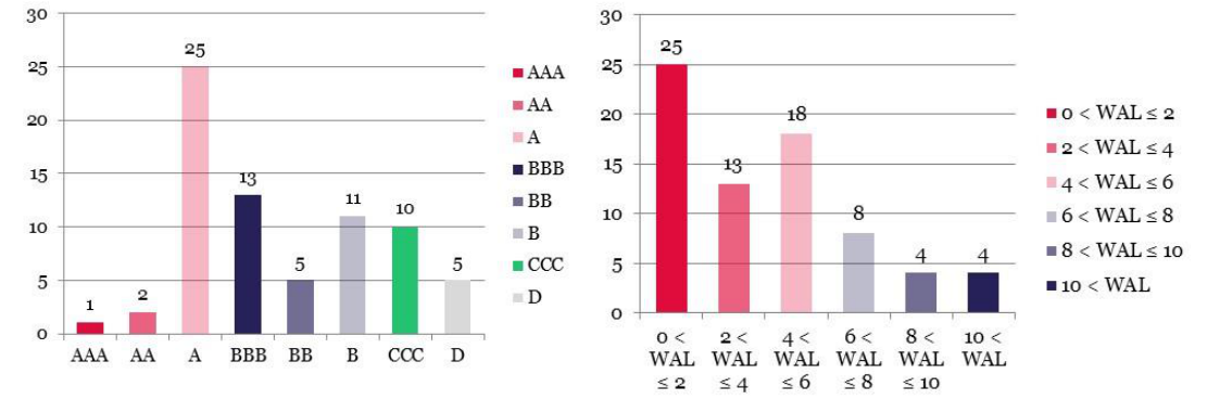
Figure 1 shows the breakdown of the exposures by rating. As one may observe, the portfolio contains very few AAA-rated tranches. Most tranches have ratings of A or BBB but there are substantial numbers of exposures rated BB, B, CCC and even default. Interpretation of ratings is, in this case, complicated by the fact that the ratings agencies apply sovereign rating caps for Spain and Portugal. If the deals involved were located in other countries, the tranches we study would no doubt bear distinctly higher ratings.
Figure 2 shows the portfolio breakdown by Weighted Average Life (WAL). The WAL for most tranches is less than 4 years. Three quarters of tranches have WALs less than 6 years. Perhaps the most representative tranche in the portfolio has a par value of EUR 50 million, a rating of BBB, and a maturity of 3 years.
3. Modelling loan losses
In this and the next section, we describe the methodology we employ to calculate risk statistics for portfolios of securitisation tranches. The methodology involves modelling the stochastic behaviour of loan pools and then building a representation of the cash flow waterfalls on top. To explain the methodology, we describe in this section how loan pools are modelled (and how we calibrate their distributions). In the next section, we describe the approach we take in modelling cash-flow waterfalls.
To model loan pools, we simulate the loss rate, θt, through time of a homogeneous pool of underlying loans, t. The methodology employed may be described as follows. Define the transformed loss rate θ̃t = Φ−1(θt) o a homogeneous loan pool. Here, Φ−1(∙) is the inverse of the standard Gaussian distribution function. Lamb and Perraudin (2008) show that, under suitable assumptions, the transformed loss rate, θ̃t, follows the Gaussian autoregressive process:
1 −√β √1 −β (1) θ̃t+1 = √βθ̃t + Φ−1(qt) − √ρ εt √1 −ρPool √1 −ρPool
Here, qt is an unconditional probability of default of individual loans (which may vary over time), β and ρPool are mean reversion and correlation parameters, and εt is a standard Gaussian shock equal to
(2) εt = −√1 −η[2] ft + η ζt
The random variables ft and ζt are standard Gaussian shocks, with ft being a factor specific to the country and industry of the securitisation pool loans, while ζt is an idiosyncratic shock specific to the securitisation in question. η is a parameter describing the weight of the idiosyncratic factor.
To calibrate these processes for each securitisation asset pool, we take the following approach. Within the RC- Capital Model software, users supply parameters for each securitisation. These parameters include an initial loss rate, θ[0], and the β, ρPool and η parameters. Users also input cumulative default rates and spreads, for maturities of 0 to 30 years which are used to calculate the unconditional pool probability of default at time t. The factor shock ft is assumed to equal a weighted sum of sector and country factors with user supplied weights.
Lamb and Perraudin (2008) provide an estimate of 0.91 for the value of β for corporate and industrial loans. This is based on aggregate data. Autocorrelation for individual securitisation pool loss rates is probably lower so we opt for a value of 0.8. The cumulative default rates used are those provided in Table 24 in Vazza et al. (2014). These go up to a time horizon of 15 years which is sufficient given the maturities of the exposures we study here. The factor shock is calculated based on a single country factor.
We choose the parameters ρPool and η based on values suggested in Duponcheele et al. (2013). In this paper the authors consider a granular securitisation pool, and suppose that a default for the ith loan depends on the value of a latent variable, Zi, which is assumed to satisfy the factor structure
(3) Zi = √ρPoolYS + √1 − ρPoolεi
Here, YS and εi are standard Gaussian shocks, with YS being a factor common to all exposures in the pool. YS, in turn, exhibits the following factor structure:
√ρ X (4) YS = YB + √1 −ρ√ρ∗ √ρPool √ρPool
Here, YB and X are standard Gaussian shocks. YB is the factor common to all the exposures in the bank portfolio and X is a factor orthogonal to YB. In order that YS be standard Gaussian, we set ρPool = ρ+ (1 −ρ)ρ∗. The authors recommend using the values ρ= 0.2 and ρ∗ = 0.1, giving a value of 0.28 for ρPool. η is analogous to the coefficient of X in (4). This is approximately equal to 0.5.
Once loss rates θ[1], … , θT for the loan pool have been calculated, the price Vt of the pool at time t may be calculated using the formula
T i T
(5) ) Vt = ∑cexp(−rt,t+ii) (∏(1 −θj)) + Qexp(−rt,t+TT) (∏(1 −θj)
i=1 j=1 j=1
Here, T is the time to maturity, c is the coupon rate, Q is the principal, and rt,t+i is the i-period interest from time t.
4. Modelling cash flow waterfalls
Having constructed a model of loan pools, one may construct a representation of the securitisation cash-flow waterfalls. Cash payments to the holders of a securitisation tranche are determined by a set of rules collectively referred to as a cash-flow waterfall. These rules describe how income on the loan pool including coupon and principal repayments and recoveries in the event of defaults are allocated to the holders of tranches of notes or bonds enjoying different levels of seniority. Contractual coupon and principal payments to the most senior tranches are paid first. Remaining monies are used to meet contractual liabilities to other tranches in order of seniority.
Given a set of cash flows and rules on the rights of different tranche holders, one may straightforwardly allocate payments among the various tranches. Hence, if one simulates pool cash flows using the approach described in the last section, by implementing the cash flow waterfall rules numerically, one may also simulate the cash flows to the tranche holders.
If one wishes to calculate risk statistics (like Value at Risk (VaR) or Expected Shortfall (ES)) for a portfolio of securitisation tranches over a holding period that exceeds the final maturity of the longest dated securitisation, then simulating the loan exposures and then using the cash flow waterfall rules to simulate the tranche cash flows is sufficient to estimate, via Monte Carlo methods, the distribution of tranche payoffs. From this risk statistics like VaRs and risk return trade-offs may be estimated.
More commonly, however, one wishes to calculate VaRs using a holding period shorter than the maturities of the securitisations in question. In this case, one may simulate cash-flows up to the investment horizon and add these cash-flows (discounted up) to the prices of the tranches at the VaR horizon. But, to do this requires that one be able to value the tranche at the horizon in question, which is generally difficult except using a numerical routine like an embedded Monte Carlo. Such embedded or nested Monte Carlo exercises are numerically infeasible since they involve a very substantial computational cost.
To avoid this difficulty of implementing nested Monte Carlos, we use a conditional regression approach similar to that used by Longstaff and Schwartz in the context of American option valuation. To be more precise, to calculate risk statistics for a securitisation with maturity T and J tranches, RC-Capital Model follows the following steps:
1. A grid of plausible transformed loss rates at the VaR horizon, t[1], is constructed. For each grid node, loss rates are simulated forward until maturity, and this process is repeated N times.
(n) be the cash flow at time t, on the jth tranche and on the nth simulation. The summed discounted
2. Let cj,t
(n) , and given by the formula cash flow at t[1], on tranche j and simulation m, is denoted DCFt,j,t[1]
T
(6)
(n) = ∑cj,i(n)Pt,t1,i DCFt,j,t1 i=t1+1
Here, Pt,t[1],i is the forward discount factor at time t for discounting a cash flow at time i back to time t[1].
(n) is defined for the loss rate history up to t[1] for simulation m:
3. For s= 1, … , S a statistic ℎt[1],s
(7)
(n) = Ht[1],s((θt: t= 1, … , t[1])) ℎt1,s
(n) , a pricing function F is By regressing the summed discounted cash flows DCFt,j,t(n)[1] on the statistics ℎt[1],s obtained, which assigns to every loss rate history up to t[1] cash flows to each of the tranches:
(8) (cj,t: j= 1, … , J, t= 1, … , T) = F((θt: t= 1, … , t[1]))
4. A further Monte Carlo is performed to calculate risk statistics at t[1] using the pricing function F.
We use 2,000,000 replications for the latter Monte Carlo. In modelling the portfolio, we assume that the underlying loans are paid off at a constant rate until maturity. For each tranche we have an estimate of the weighted average life (WAL), calculated assuming a constant prepayment rate, and taking into account the payment structure of the securitisation. We choose a value for the maturity of the underlying loans that results in a WAL equal to the sum of the WALs of the tranches, weighted by their value as a fraction of the value of the entire deal. Given the linear amortisation schedule, the maturity should be set to twice this weighted sum. We obtain yield data for the underlying loans from Bloomberg.
5. Results
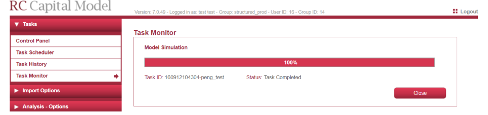
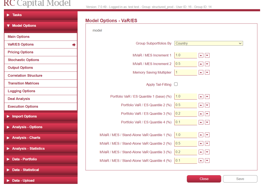
In this section, we present an analysis of our example SME-loan-backed securitisation portfolio implemented using RC-Capital Model. Figure 3 shows the task monitor window of RC-Capital Model when the simulation is performed. Throughout this section, unless otherwise specified, all VaRs are calculated over a horizon of one year and at a 99.9% confidence level, and are presented as a fraction of the current value. Multiple confidence intervals can be specified in the software, as shown in Figure 4, along with other model options.
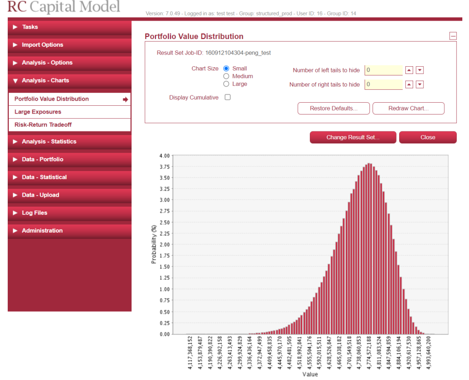
Figure 5 shows a histogram of the total value of the securitisation portfolio at the one year horizon. Note that the distribution is in monetary terms and not in returns. Its left skewed appearance reflects the significant influence of downside credit risk.
A summary of the results is presented in Figure 6. As well as the left skew referred to above, the distribution exhibits slight positive excess kurtosis. The 99.9% VaR as a fraction of the expected forward value of the portfolio is 8.20%, just slightly higher than the Basel I capital percentage of 8%. The Expected Shortfall (ES) is, of course, higher but not very substantially so.
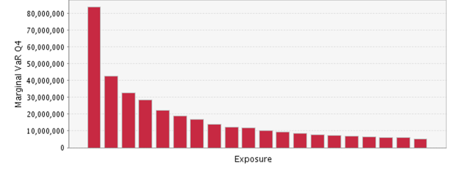
We now consider risk statistics for individual exposures considered as part of the wider portfolio. Figure 7 shows the 20 exposures for which the marginal VaRs are largest. The largest MVaR is €84 million, more than 20% of the total portfolio VaR. The top two exposures are both from BBVA-originated deals, and were assigned credit ratings of B- and BBB respectively. After the top ten MVaRs, the risk on individual exposure is quite low.
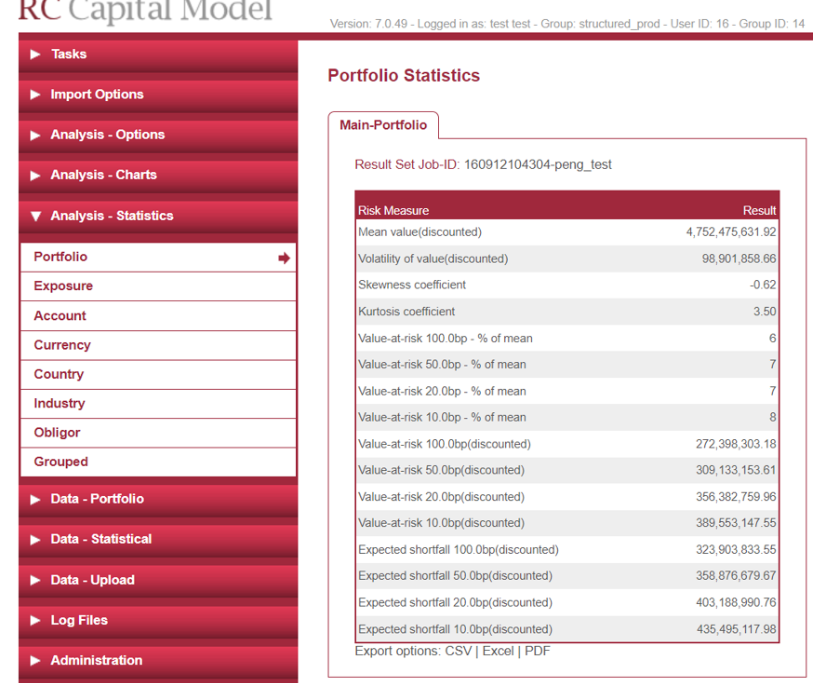
Note: The table presents summary statistics for the portfolio, calculated using Monte Carlos. All figures are given in Euros and are discounted to the present.
6. Comparison with AFA
In this section, we benchmark the marginal VaRs obtained from RC-Capital Model to those calculated using the Arbitrage Free Approach (AFA) described in Duponcheele et al. (2013). We begin by giving a brief summary of the AFA. The latter is a stylised analytical measure of the marginal VaR of a securitisation exposure suitable for use within a regulatory capital framework.
Here, we employ the AFA as a benchmark for the more realistic (less stylised) approach possible if one employs our Monte Carlo methodology. Specifically, the Monte Carlo approach permits one to use a realistically complicated representation of the cash flows on pool assets and securitisation tranches. It also permits one, if one wishes, to use a more general factor and hence correlation structure for the underlying risks.
Note that the scope to employ a more general factor structure is slightly less important when one is examining a portfolio comprising a single asset class (here, SME-loan-backed deals) within effectively a single geographical region (here Spain and Portugal). With more general portfolios (for example, comprising Spanish and UK deals), a richer correlation structure would be appropriate.
We begin by defining the parameters used in the calculation of the AFA. We consider a securitisation tranche with attachment and detachment points A and D. Let M be the maturity of the securitisation, and let pdM and LGD be the M-year probability of default and the loss given default on the pool assets. We recall from Section 3 that ρ= 0.2, ρ∗ = 0.1 and ρPool = 0.28. The expected loss for the tranche may be calculated using equations (9)- (13).
(1 −A) × ELSenior(A) −(1 −D) × ELSenior(D) (9) EL(A, D) = D−A
(10) ELSenior(X) = LGD× N̅[2] −X× PDTrancℎe(X) 1 −X
(11) N̅[2] = N[2](N−1(PDM), N−1(PDTrancℎe(X)), √ρPool)
N−1(PDM) −N−1 ( X LGD) √1 −ρPool (12) ) PDTrancℎe(X) = N( √ρPool
(M−1)γ ) (13) PDM = N(N−1(pdM) + √M γ is a risk-premium parameter, which, according to Bohn (2000), should be assigned a value between 0.3 and 0.5. We use a value of 0.3 in our calculations. N is the normal cumulative distribution function and N[2](, , ρ) are is the bivariate normal cumulative distribution functions, with correlation ρ.
To calculate the marginal VaR using the AFA, we require the stressed M-year probability of default on the pool assets PDα,M. Duponcheele et al. (2013) provide two ways of calculating PDα,M. According to the first method, PDα,M is calculated using the formula
N−1(PDM) −√ ρ M N−1(α) (14) PDα,M = N √1 − ρ ( M )
Here, α is the confidence interval, taken here to be 0.001. This is the approach followed here.
In the second method, PDα,M is chosen so as to ensure that the total capital requirement for all the tranches of a securitisation is equal to the IRBA capital requirement for the underlying loans, KIRB (see Basel Committee on Banking Supervision (2006)). This implies that
(15) PDα,M = KIRB LGD + PDM
∗ is given by the To obtain capital estimates, we replace PDM by PDα,M and replace ρPool with ρM∗ , where ρM formula
(1 −ρ)ρ∗ + (M−1)ρPool (16) ∗ = ρM (1 −ρ) + (M−1)
We, thereby, obtain MVaR(A, D) instead of EL(A, D). For the M-year probability of default pdM, we use the cumulative default rates provided in Table 24 in Vazza et al. (2014) and linear interpolation.
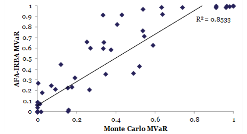
Figure 8 shows how the marginal VaRs calculated using the Monte Carlo approach compare to the marginal VaRs calculated using the AFA. Here PDα,M is calculated using (14). The linear regression lines and R[2]’s are shown. The high R[2] may partly be attributed to clustering, with low risk and high risk tranches being assigned MVaRs close to 0 and 1 respectively, regardless of the calculation method, but with the two MVaR calculations differing noticeably for tranches that fall into neither of the above groups.
Figure 9 shows a similar comparison, with PDα,M calculated using (15). The two sets of results are similar, with
(15) AFA producing slightly higher MVaRs.
Figure 8: AFA marginal VaR versus Monte Carlo MVaR
Table 1 presents the results of regressions of differences between the AFA MVaRs and the Monte Carlo MVaRs (that appear in Figure 9) on different exposure characteristics. The differences depend negatively on the duration of the securitisation and positively on the tranche attachment point. This shows that the AFA overestimates the contribution to risk of duration and under-estimates the effect of attachment point compared to the more realistic Monte Carlo model. The default profile dummy variable employed in the regression takes a value of unity when the pool default probability profile is riskier and zero otherwise. The coefficient for this variable is positive, as expected, and statistically significant.
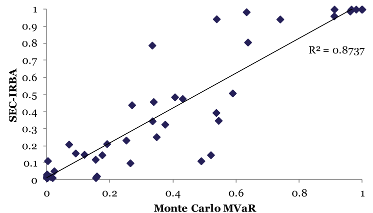
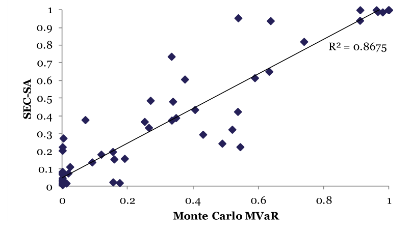
Finally, we compare, in Figure 10 and Figure 11, the Monte Carlo marginal VaRs to SSFA capital charges. The SEC-IRBA and SEC-SA capital charges are calculated according to the rules specified in Basel Committee on Banking Supervision (2014). The SEC-IRBA capital charges are slightly lower than the Monte Carlo MVaRs for some exposures. This reflects, in part, the firm-size adjustment for SMEs used in the IRBA. But, the regulatory and Monte Carlo MVaRs are generally positively correlated.
| Variable | Estimate | SE | t-stat | p-value |
|---|---|---|---|---|
| Intercept | 0.02 | 0.05 | 0.48 | 0.64 |
| Deal duration | -0.02 | 0.01 | -1.44 | 0.16 |
| Attachment point | 0.02 | 0.05 | 0.37 | 0.71 |
| Default profile | 0.09 | 0.03 | 2.93 | 0.00 |
Note: The table shows the results obtained by regressing the difference between the AFA marginal VaR and the Monte Carlo marginal VaR on the duration of the deal, the attachment point of the tranche and a dummy variable for the default profile. In our analysis two default profiles are used in the Monte Carlo simulation, the default profile variable is set to 1 for exposures to securitisations assigned to the riskier of the two default profiles, and 0 otherwise.
7. Conclusion
The models presented in this note constitute a toolbox of rigorous techniques for analysing securitisation portfolio risk. As such, they permit the user to analyse with confidence the risks in holding securitisation exposures, to understand the risk return trade-offs for such exposures and appropriate levels of capital. The models presented include a flexible Monte Carlo-based framework in which multi-period securitisations with complex cash-flow waterfalls may be represented and a simple, stylised analytical model, the Arbitrage Free Approach (AFA) (as proposed by Duponcheele, Perraudin and Totouom-Tangho (2013)).
We show in a case study of Spanish and Portuguese SME-loan-backed securitisation tranches that our Monte Carlo model provides intuitively reasonable risk measures. Using it, we calculate Marginal Value at Risk (MVaR) measures and show that they are correlated across individual exposures with familiar risk drivers such as attachment point, maturity and agency rating. When implemented under comparable assumptions, the Monte Carlo-based capital numbers also exhibit high cross-sectional correlations with those implied by the AFA and with regulatory capital.
Differences between the capital implied by the Monte Carlo and analytical models reflect the more realistic modelling of the cash-flow waterfall possible within the former and differences in the modelling of pool loan defaults. (This modelling is multi-period in the Monte Carlo model and single-period in the stylised models.)
8. References
Basel Committee on Banking Supervision (2006) “International Convergence of Capital Measurement and Capital Standards,” Bank for International Settlements, June, (also known as BCBS 128), available at: http://www.bis.org/publ/bcbs128.pdf
Basel Committee on Banking Supervision (2014) “Revisions to the securitisation framework,” Basel III document, Bank for International Settlements, December, (also known as BCBS 303), available at: http://www.bis.org/bcbs/publ/d303.htm
Bohn, Jeffrey (2000) “An Empirical Assessment of a Simple Contingent-Claims Model for the Valuation of Risky Debt,” Journal of Risk Finance, Vol. 1, No. 4, pp. 55-77.
Duponcheele, Georges, William Perraudin and Daniel Totouom-Tangho (2013) “Maturity Effects in Securitisation Capital: Total Capital Levels and Dispersion Across Tranches,” BNP Paribas mimeo, September, available at: http://www.riskcontrollimited.com/insights/maturity-effects-in-securitisation-capital-totalcapital-levels-and-dispersion-across-tranches/
Lamb, Robert and William Perraudin (2008) “Dynamic Default Rates,” available at: http://www.riskcontrollimited.com/insights/dynamic-default-rates/
Vazza, Dianne, Nick Kraemer, Nivritti Richhariya, Abhik Debnath and Mayur Sangoi (2014) “Default, Transition, and Recovery: 2014 Annual Global Corporate Default Study And Rating Transitions,” Standard and Poor’s, April.
Risk Control Limited 13-14 Dean Street London W1D 3RS +44 (0)203 307 0730 www.riskcontrollimited.com
Notes
[1] This note was prepared by Jozsef Kutas and William Perraudin.