Regulatory and 'Economic' Solvency Standards for Internationally Active Banks

Research Paper

Regulatory and “economic” solvency standards for internationally active banks

Date: 2002 Reference Number:2/1

Regulatory and “economic” solvency standards for internationally active banks

Patricia Jackson William Perraudin and Victoria Saporta

e-mail: patricia.jackson@bankofengland.co.uk william.perraudin@riskcontrollimited.com victoria.saporta@bankofengland.co.uk

Summary

The Basel Committee is currently engaged in designing a new Accord on the capital adequacy of internationally active banks that will supersede the original 1988 Accord. Under the old Accord internationally active banks in G10 countries are required to hold broad and narrow capital that is no less than 8% and 4% respectively of their risk-weighted assets. While exposures to banks, sovereigns and mortgage assets are differently treated, the bulk of banks’ private sector assets are subject to the same capital charges no matter how risky they are. In framing the new Accord, the Basel Committee intends to make capital charges on different exposures much more risk-sensitive.

A major question confronting regulators is how high the overall average level of capital charges for representative banks should be. The 8% in the original Basel Accord was chosen on the basis that this was the minimum level of capital observed among banks that were perceived to be following best industry practice. When capital charges are being redesigned as part of the preparation of the new Accord, it is natural to consider what current levels of regulatory capital imply for financial stability and to what extent these are a binding constraint on banks.

This paper employs a standard credit risk model to investigate the survival probabilities implied by the current minimum level of narrow regulatory capital (subordinated debt included in the wider definition does not affect survival probabilities). In particular, for corporate loan portfolios with representative quality distributions, we calculate the likelihood that the banks holding the portfolio would survive over a one-year horizon if their capital were at the regulatory minimum. The model employed is a simplified version of the widely used CreditMetrics approach, developed by JP Morgan.

We then compare the survival probabilities implied by minimum levels of regulatory capital with those levels of ‘economic’ capital that internationally active banks actually hold. We do this in two ways. First, we again employ CreditMetrics calculations. Second, we examine the historical survival rates associated with the ratings that banks receive from the main rating agencies. This latter examination is complicated by the fact that, in many cases, banks’ agency ratings are boosted by market expectations that the authorities will provide support if they experience difficulties. To get around this problem, we calculate, using an econometric model, what ratings banks would have if they were not expected to be able to obtain support.

We conclude from our calculations that the one-year survival probability or solvency standard implied by the current Basel Accord minimum capital levels is between 99.0% and 99.9% depending on the quality of the corporate loan book used. Our investigation of the solvency standard implicit in the ‘economic’ capital levels that internationally active banks actually hold suggests that it is substantially higher than 99.9%.

Having investigated the relation between the survival rates implied by regulatory minimum capital levels and by the capital levels that banks actually hold, we ask a further question: why do banks make such apparently conservative capital decisions, selecting economic capital that significantly exceeds the regulatory minimum? It is difficult to answer this question conclusively but we argue that the evidence is at least consistent with one explanation, namely that banks are obliged to maintain higher capital levels in order to obtain access to certain wholesale markets, most notably the swap market, participation in which is a prerequisite for operating a modern large-scale, internationally active bank. To make the case that market discipline of this kind is an influence on banks’ choices, we show that the volume of banks’ swap liabilities conditioning on bank size is significantly correlated with the bank’s credit rating. Large international banks wanting to deal in significant swap volumes appear to have to maintain high ratings.

The main implication of our analysis is that maintaining capital minimum regulatory capital levels in the new Basel Accord at levels similar to those that apply under the 1988 Accord would not act as a major constraint on most internationally active banks since they already operate on higher ‘economic’ solvency standards than those implicit in the Basel regulatory minimum. While different reasons might be adduced for why banks adopt a relatively conservative approach in their capitalsetting decisions, one possibility that seems consistent with data on swap market volumes is that the need to maintain access to certain wholesale markets, which is crucial to operating a large bank, necessitates a fairly stringent ‘economic’ solvency standard.

Introduction

In the current system of bank regulation within G10 countries, the single most important decision faced by regulators is the choice of the overall average level of bank capital. Under the 1988 Basel Accord capital charges were set at 8% of private sector exposures with adjustments for mortgages and bank assets. (A brief account of the capital rules in the 1988 Accord is provided in the appendix on page 36). The Basel Committee is currently designing a new, risk-sensitive Basel Accord under which levels of bank regulatory capital will depend in a detailed way on the risks of the assets that the bank holds.

This paper sheds light on the implications of different levels of bank capital by studying the survival probabilities for representative banks over given horizons (or ‘solvency standards’) that they imply. First, using a ratings-based credit risk model, we assess the solvency standard implied by the 1988 Basel Accord minimum capital requirements. This is interesting because the Basel Committee has decided that, in a future New Accord, the current minimum level of capital in the system should be maintained (BCBS (1999) and BCBS (2001)). We find that the confidence level implicit in the 1988 Accord is equivalent to saying that representative banks will survive over a one-year horizon with a probability of between 99.0% and 99.9%.

Second, several banking associations have contended that the Basel Accord should not seek to maintain the current level of minimum capital because this imposes efficiency costs on the industry. Their contention raises the question of whether large internationally active banks could plausibly seek to operate at lower solvency levels than implied by the current Accord. We examine this issue by investigating the ‘economic’ solvency standards that banks themselves adhere to in choosing their levels of economic capital. Our investigation is based, first, on a statistical analysis of the agency ratings that banks receive and second, on credit risk model calculations. The statistical analysis is designed to adjust agency ratings for official or other support. We conclude that banks generally employ solvency standards higher than 99.9%.

This suggests that in normal times, the 1988 Basel Accord does not act as a binding constraint on the capital choices of representative international banks.(1) The implication must be that market discipline induces banks to hold capital in excess of the regulatory minimum. To document how this may come about, we investigate the access that banks have to important markets. Our analysis, which is suggestive rather than conclusive, consists of showing that, after one has controlled for bank size, there remains a strong association between swap volumes and credit quality. This is consistent with the plausible argument that banks are obliged to maintain high levels of capital in order to obtain sufficient access to credit markets, including swap and interbank, for their current business. Access to such markets is a prerequisite to modern banking operations.

Despite their importance, few studies have examined the issues dealt with in this paper. Ronn and Verma (1989) and Nickell and Perraudin (2001) examine banks’ default probabilities using equity-based models. Kiesel, Perraudin and Taylor

(2001) measure default probabilities of representative banks using a ratings-based model similar to that employed here. None of these papers has focused on or contrasted the different solvency standards imposed by regulators and those chosen by banks themselves, however. A paper that in some ways resembles this one is Carey (2001), which conducts calculations of default likelihood for banks under different assumptions about capitalisation. His paper employs a default-mode approach in that banks are assumed to be insolvent only if a sufficient fraction of their loans have defaulted. Deterioration in the credit quality of loans that do not default is not assumed to matter in his treatment. In practice, however, banks reduce capital to create provisions against weakened loans even when the borrowers have not defaulted.

The article is structured as follows. Section 2 provides background to our analysis, describing relevant aspects of the current review of the Basel Accord. Section 3 examines the solvency standard implied by the regulatory capital minimum required by the 1988 Basel Accord using a credit risk model. Section 4 investigates the

____________________________________________________________________ __________

(1) In periods of recession, on the other hand, the regulatory requirements may bind.

solvency standard that international active banks currently employ using a combination of credit risk model calculations and analysis of agency ratings obtained by banks. Section 5 studies the association between banks’ access to the swap market and their credit standing.

2 Background

The Basel Committee is currently revising the 1988 Basel Accord, which sets minimum capital standards for significant banks worldwide. The Accord was originally agreed by the G10 and Switzerland but has since been adopted by more than 100 countries. In January this year, following two years of deliberation, the Committee set out detailed proposals for a new Accord (BCBS (2001)). Pillar 1 of the revised Accord will deliver new risk-based requirements for credit risk and a new charge for operational risks. Pillar 2 will set requirements for supervisory review and Pillar 3 will set new bank disclosure standards.

The prevalent view among regulators is that the role of capital requirements is to reduce, although not completely eliminate, the likelihood that banks will fail. The need to protect small investors and the undesirable systemic effects that bank failures may provoke are commonly advanced as justifications for the imposition of capital requirements. On the other hand, excessively high capital requirements may impose efficiency costs on the financial sector. To calibrate capital requirements, one needs to balance the trade-off between these two effects in order to arrive at the appropriate solvency standard (defined as one minus the probability of default for a representative bank) that the requirements should attempt to deliver.

Early on in the process, the Basel Committee decided that the current level of minimum capital in the system should be maintained (BCBS (1999) and BCBS (2001)). Some justification for this approach is provided by the fact that even since the introduction of the 1988 Accord, there have been a large number of banking crises. Of the sample of 53 countries studied by IMF (1998), four Basel member countries and 20 non-Basel member countries had financial crises in the post-1988 period. The Asian and Japanese banking crises have further underlined the substantial costs imposed by fragile financial systems. In combination, these experiences are likely to have contributed to the Committee’s reluctance to see any erosion in minimum capital.(2)

In this article, we do not express a view on the appropriateness of the Basel Committee’s decision to maintain the current average level of bank capital. Instead, we examine the solvency standard implicit in this decision and compare it with the solvency standards adopted by the banks themselves. Having concluded that the Basel Accord regulatory minimum is not a binding constraint for average internationally active banks given their current levels of capital, we examine how the desire to obtain access to markets like the market in swaps may induce banks to maintain high capital levels.

It is important to realise that even if the Basel Accord regulatory minimum is not at present a constraint on most internationally active banks, the level at which this minimum is set is nevertheless very important. With broad public safety nets in some countries, banks may be able to operate close to any regulatory minimum and could chose to do so. Even without such a safety net, banks that can rely on small depositors for funding may be able to operate at the minimum — even if that is set at a very low level. Furthermore, even if the regulatory minimum does not generally bind for a given bank, it will provide a useful trigger for regulatory actions of different kinds if the credit quality of the bank’s loan book and capital ratios were to deteriorate.

____________________________________________________________________ __________

(2) The relatively small number of observations, the changes in bank behaviour (for example increasing use of risk management and securitisation) and the changes in the lending environment that banks face make it difficult to compare the likelihood of banking crises before and after the 1988 Accord systematically. But the post-1988 experience is consistent with the preference of the Basel Committee at least to maintain the level of capital in the system.

3 The solvency standard delivered by the current Accord

3.1 A ratings-based credit risk model

The current Basel Accord sets a minimum capital requirement for exposures to private sector borrowers (other than inter-bank or residential mortgages) of 8%, of which 4% must be equity or reserves. The remaining 4% may be made up of subordinated debt or general provisions. However, the solvency standard depends on the level of equity and reserves. Subordinated debt will not prevent a bank from failing although it may in part absorb losses after failure and therefore help depositors.(3)

To assess the confidence interval delivered by the current Accord, one should, therefore, focus on the 4% consisting of equity and reserves. For a bank with a particular portfolio of corporate exposures, and using a suitable credit risk-model, it is possible to estimate the confidence interval delivered by the 4% — ie the number of occasions for which losses on the portfolio would exceed the 4% equity.

In this study, we perform calculations of this kind using a credit risk model based on the widely employed CreditMetrics methodology (JP Morgan (1997)). Although this approach is widely used in the industry, one should note that the limited evidence available on its out-of-sample performance (see Nickell, Perraudin and Varotto (2001)) suggests that it may overestimate confidence levels.(4) Our results should be interpreted with this in mind.

____________________________________________________________________ __________

(3) Even in this, subordinated debt is often not enough. US evidence shows that over the period 1980-94 the average cost of bank failures to the FDIC as a percentage of the failed banks’ assets was around 27% (FDIC (1998)).

(4) The most obvious reason why CreditMetrics-style calculations might underestimate risk is that they leave out certain forms of risk such as, for example, operational risks. However, when banks default, this is mostly the result of deterioration in the value of their credit exposures which CreditMetrics models do capture. In our view, CreditMetrics omits certain aspects of credit risk, most notably spread risk, systematic risk in recoveries that is correlated with deterioration in credit quality elsewhere in the book. In other studies, we have examined these additional types of credit risk (see Kiesel, Perraudin Taylor 2001 and Hu and Perraudin 2001).

We suppose throughout that the bank’s book consists of corporate exposures. This approach is dictated by the fact that data on credit quality distributions is only publicly available for corporate loan books. Corporate lending tends to form the greatest part of total lending by internationally active banks in most countries that are members of the Basel Committee, although in some countries and for some large and complex financial institutions in others, retail lending is also important (see Table F below). The implications of omitting information on the credit quality of non-corporate assets are discussed briefly at the end of this section.

The CreditMetrics approach reduces credit risk for individual exposures to the possibility that the rating of the exposure will change or the issuer will default before a fixed, future point in time, and that, if default occurs, the value recovered will be random. The future value of an exposure, conditional on its future rating, is assumed known (ie no allowance is made for spread risk). The distribution of credit losses generated by the model depends crucially on the degree of correlation between ratings changes for different obligors.

More formally, suppose there are J possible rating categories with category J representing default and rating 1 being the highest credit quality category, AAA. Consider a portfolio made up of M credit exposures with ratings Rm,t at date t. Suppose that the path of interest rates is deterministic so that the value of each exposure, Vm,t , at any date t is known, conditional on knowing the rating of the

exposure at that date. At date t, the random future value of the portfolio of credit exposures at date t+1 may be written as:

M Vm,t+1(Rm,t ). (1) ∑ m=1

To obtain risk measures for the portfolio, ratings-based models like CreditMetrics, one may simulate changes in ratings and calculate statistics of the future portfolio value. The most common statistic to calculate is the Value at Risk (VaR) of the portfolio. This is the loss (measured as a deviation from the mean future value of the portfolio) that is exceeded on some fraction α of occasions if the portfolio is held for a fixed period such as a year. The parameter 1-α corresponds to what we refer to elsewhere in this paper as the confidence level or solvency standard. If the bank sets its capital equal to the VaR, then α equals the probability that it will default over the horizon of the VaR calculation.

Under the above assumptions, the task of estimating VaRs reduces to one of simulating changes in ratings for each of the M exposures over the horizon of the VaR calculation. CreditMetrics assumes that the probabilities that an exposure with rating i at date t will be rated j at date t+1 is a constant πi, j . Let the matrix of which

the element in the ith row and the jth column equals the probability πi, j be denoted Π ≡ [πi, j ]. This matrix is commonly referred to as the rating transition matrix.

Knowing the probabilities that the rating will change from i to j for all possible i and j, and the values that the exposures will have conditional on particular ratings now and in the future means that one knows the entire distribution of the future value of each individual exposure. What one does not know, however, is the distribution of the portfolio value since this will also depend on the degree of dependence between ratings changes on different exposures, for example the level of correlation between rating changes.

The approach taken by CreditMetrics is to suppose that ratings changes for individual exposures are driven by realisations of normally distributed latent variables. More precisely, whether the rating at date t+1 of an exposure m rated i at t is rated j at t+1 is determined by whether a latent variable Xm,t+[1] falls into the jth − ∞, Z Z Z Z , Z , interval among the set of J intervals: ( i1, ], ( i1,, i,[2] ] , …, ( i,J−[2] i,J−[1] ] Z ∞ where the ( i,J−[1], ) Zi, j are fixed cut-off points. Since the latent variables are

assumed normally distributed, the probabilities of moving from rating i to rating j may be expressed as:

πi, j ≡ Φ(Zi, j )− Φ(Zi, j−1). (2)

The usefulness of transforming the ‘discrete problem’ of simulating changes in rating from an initial rating i to a terminal rating that is one of j=1,2,...,J possible future values at date t+1 into a ‘continuous problem’ of simulating normally distributed latent variables is that one may introduce correlations between changes in different ratings in a simple fashion by allowing the latent variables to be correlated. In general, this may be achieved by supposing that each latent variable is a weighted sum of common factors plus an independent, idiosyncratic error term. When there is a single factor we may express this as:

X m,t+1 = βm ft+1 +εm,t+1 (3)

If X m,t+[1]is to be standard normal (ie zero mean and unit variance) as is assumed above, it must be the case that Vart (εm,t+[1] ) = 1−βm . The correlation between the

latent variables for two different exposures, X m,t+[1]and X k,t+[1] is then βm ×βk . In

our simulations below, we shall assume that this correlation is the same for all pairs of exposures, ie, are constant cross-sectionally.(5)

Having made the above assumptions, one may simulate correlated rating changes by repeatedly generating correlated normal random numbers, valuing the exposures conditional on each set of ratings and hence calculating the value of the portfolio for each realisation of the random numbers. This yields an estimate of the distribution of the future portfolio value from which one may derive risk measures like VaRs and (subject to some rule linking risk measures to capital) the implied capital numbers the institution should hold.

The crucial parameters in calculations of this type are, therefore: (i) the rating transition probabilities, πi, j ; (ii) the degree of correlation between the latent variables driving different rating transitions; and (iii) spreads that are used in calculating the exposure values conditional on different ratings, Vm,t .

____________________________________________________________________ __________

(5) In practical applications of CreditMetrics-like models on actual portfolios, factors are typically assumed to be weighted averages of industry and country equity indices with weights chosen to reflect the industry and country exposures of individual obligors. The degree of correlation between pairs of exposures then varies across obligors depending on the factor correlations and the weights. For the purpose of analysing capital requirements, it is sensible to simplify by assuming the same level of correlation across all exposures.

3.2 Calculation results

The calculations we show below are based on three different credit quality distributions for a corporate portfolio (see Table A). The first two quality distributions are representative portfolios from a Federal Reserve Board survey of large US banks reported in Gordy (2000).(6) The average portfolio represents the average distribution of value-weighted credit exposures across internal grades mapped to Standard and Poor’s rating grades for all the banks surveyed by the Federal Reserve. The high-quality portfolio is, according to the Federal Reserve Board, representative of the higher-quality distributions found in the survey. The third is based on the internal rating distribution (as per year-end 1999) of Deutsche Bank, one of the few banks to release information of this kind in its annual report.

Table A: Portfolio distributions of credit quality

Average quality – US High quality – US High quality – European (%) (%) (%) AAA 3 4 - AA 5 6 32 A 13 29 19 BBB 29 36 26 BB 35 21 18 B 12 3 4 CCC 3 1 1

Table B contains our baseline calculations for these three portfolios. The assumptions we adopt in making these calculations are as follows:

(1) The portfolio contains 500 pure discount exposures with equal par values and maturities of 3 years.

(2) The time horizon of the calculation is one year (ie losses over one year periods are captured in the VaR calculation).

____________________________________________________________________ __________

(3) The ratings transitions matrix employed is that estimated for US industrials by Nickell, Perraudin and Varotto (2000) (using Moody’s historical data from 1970 to 1998).

(4) The recovery rate in the event of default has a Beta distribution(7) with mean 50% and standard deviation 25%.

(5) The spreads for different ratings categories are the averages for US industrials reported by Kiesel, Perraudin and Taylor (2001), based on Bloomberg data in the period 1991 to 1998.(8)

(6) Correlations between the latent variables generating ratings changes are assumed to be 20%.

The figure used for the correlation between the latent variables generating ratings changes makes a substantial difference. As mentioned above, common industry practice in applying CreditMetrics is to employ correlation coefficients for weighted sums of equity indices where the weights are selected according to the industry or country of the obligors in question. This often leads to fairly high correlation coefficients of the order of 15% or 20%. Varotto (2000) analyses correlations in a large database of eurobonds returns and suggests that the average correlation is around 9% or 10%. However, to generate correlations of this order for bond returns requires that the correlation parameters for the underlying latent variables be about 20%.

The assumed recovery rate of 50% is close to the recovery rate of 51% that Moody’s have found in their data on senior unsecured bond defaults. One may note that it is

____________________________________________________________________ __________

(7) The Beta distribution is a standard, continuous two-parameter distribution with a density of the form f(x)= λxα-1(1-x)β-1 for 0<x<1 and α>0, β>0 and where λ is chosen so the density integrates to unity. It is widely used to model recoveries because it has as support the interval [0,1] and recoveries are always positive and almost always less than 100%.

(8) Each rating category is associated with a single spread. The model presumes that exposures are allocated to a discrete number of rating categories and that ratings (and hence values) evolve according to a Markov chain. While the latent variables used to model correlations have a continuous distribution, this does not imply that credit quality is assumed to be continuous.

commonly argued that recovery rates on bank loans are higher. Carty and Lieberman (1996), for example, find that recoveries on senior secured bank loans are 71% while those on senior secured, senior unsecured and subordinated bonds are respectively 57%, 46% and 34%. Asarnow and Edwards (1996) estimate average recoveries on bank loans to be 65%.

Despite these studies, we believe a lower recovery rate is appropriate for three reasons. First, the estimates of average recovery rates generally cited either are for relatively high seniority loans (see Carty and Lieberman (1996) who use senior secured loans) or are based on calculations of actual discounted cash recoveries made by banks rather than on market values at default (see Asarnow and Edwards (1995)). In either case, this yields higher average recovery rate estimates than one would obtain than for average loan recovery rates calculated on a market value basis.(9) Second, Hu and Perraudin (2001) show that average recovery rates are negatively correlated with aggregate default rates. (To put it another way, loss rates and default rates tend to rise together in economic downturns.) Hence, one should employ relatively low recovery rates in VaR calculations, since, conditional on being in the tail of the loss distribution, average recoveries are likely to be low. Third, confidential survey evidence from G10 banks suggests that average recovery rates for unsecured loans are lower than those suggested by the above-cited academic studies. Recovery rates on secured loans, reported also in the same study, vary substantially across banks making it difficult to establish a reliable central tendency. In any event, anecdotal evidence suggests that the fraction of collateralised loans as a percentage of all loans in banks’ large corporate portfolios is probably small.

____________________________________________________________________ __________

(9) This is obvious if high-seniority loans are employed. To see that recovery estimates based on discounted cash flows are higher than those based on market values at default, one should note that the market value should equal the expected discounted cash flows in which the discount factor is boosted by a risk premium.

Table B: Baseline calculations

Confidence level associated with 4% credit losses Average quality – US High quality – US High quality – European

98.95 99.86 99.91

The base-line calculations presented in Table B indicate that the current Basel Accord will deliver a solvency standard of around 99.9% for a bank with corporate loans similar to the high-quality US distribution and the one European bank. If one compares this with S&P one-year average default rates for the period 1981-99, it is equivalent to the upper end of the BBB rating category.(10) The confidence level of 98.95% for the average-quality US book is significantly lower and is equivalent to that delivered to a BB rating.(11) (12)

For banks with even lower quality portfolios (for example, those operating in a more volatile market in which corporate defaults are more frequent or specialising in rather higher risk loans) the confidence level will, of course, be lower yet. Hence, some emerging market supervisors have applied much higher minimum capital levels than the Basel 8%. For example, in Argentina the minimum is 11.5% plus 1% if the bank is exposed to market risk, while in Singapore the minimum is 12%. In the United Kingdom, bank-specific minimum capital levels termed trigger ratios

____________________________________________________________________ __________

(10) Table 3 in ‘Greater risks means more defaults in 1999’, Standard and Poor’s, 25 January 2000. There are differences between the annual default rates based on the experience of Standard and Poor’s and Moody’s. The one-year average default rates for bonds rated AAA, AA, A, BBB, BB, B are 0.00, 0.08, 0.08, 0.30, 1.43 and 4.48% based on Moody’s data for the period 1920-99 and 0.00, 0.01, 0.04, 0.21, 0.91 and 5.16% based on S&P data for the period 1981-99 respectively. One important reason for the difference in one-year default rates between the two sources is that, unlike the data by S&P, the Moody’s data cover the Great Depression. In the rest of the paper, for consistency, when we translate solvency standards to external ratings or vice versa, we employ the one-year average default rates reported in the study by S&P. Nevertheless, one should be cautious in interpreting differences in default rates. Cantor and Falkenstein (2001) provide evidence that significance levels of apparent differences are not great.

(11) Under the above assumptions, the average quality US bank would need to hold 7.88% (compared with the 4% Basel minimum) to achieve the 99.91% confidence level delivered by the Basel minimum for the European bank.

(12) As already noted, these calculations are predicated on a mean recovery rate of 50%. If the calculation were repeated for a 70% recovery rate (ie 30% loss given default or LGD) the results would be 99.79%, 99.99% and 99.99% for the average and high-quality US banks and the European bank, respectively. But as discussed earlier, we believe that this is too high a recovery rate for the whole of a bank’s portfolio.

have been set to reflect the risk profile of the bank in question enabling higher requirements to be set for higher-risk banks.

3.3 Diversification, default versus economic loss, and horizon

It is likely that some banks will not be as diversified as assumed in the baseline calculations. We have therefore examined the effect of more concentrated portfolios. The base-line calculations were repeated for the three quality distributions but ensuring that, in each case, 10% of the exposures contributed 40% of the portfolio value – see Table C. This reduces the confidence levels but the effect is slight, except for the average-quality US book.

Table C: Calculation for less diversified portfolios

Average quality – US High quality – US High quality – European 98.75 99.82 99.90

All these calculations are based on the economic loss a bank would suffer if it experienced downgrades in the quality of its loans as well as outright defaults. Some of the economic capital models that banks employ only count losses associated with realised defaults (eg, CreditRisk+, CSFP (1997)). If defaults alone are the basis for the calculated VaRs, the confidence level delivered by the current Accord is increased for all portfolios (see Table D below), but more so (in terms of basis points) for the lower quality one. This is to be expected, given that the discrepancy between the capital delivered by a typical credit risk model applying an economic loss approach and that by the same model applying the default mode approach is larger, the greater the probability of credit deterioration. High-quality assets have, by definition, a higher likelihood of a downgrade than lower-quality assets.

Table D: Baseline calculations – default basis

Average quality – US High quality – US High quality – European 99.34 99.95 99.96

But a calculation that only captures defaults would call into question another aspect of the base-line calculation, which is the use of a one-year horizon for losses. The average length of a loan for a UK or US bank is probably closer to three years. There would therefore be an argument for adopting a three-year horizon for losses, which would substantially reduce the calculated confidence intervals. See Table E below for the results under both the economic loss and the default-basis assumptions.(13)

Table E: Baseline Calculations – three-year time horizon

Economic loss Average quality – US High quality – US High quality – European 95.80 99.22 99.53 Default mode Average quality – US High quality – US High quality – European 97.35 99.77 99.86

If it can be assumed that a bank can take some action (to reduce the loan book or raise new capital) then a shorter horizon of a year may be appropriate. But a oneyear horizon is not consistent with a default-mode calculation of the confidence level. In any year, a bank must be able to withstand not just defaults but also specific provisions (or reserves) against loans that have deteriorated (that are deducted from capital). It is also the case that the weakening in the quality of a loan book will lead to losses in several consecutive years and a bank may not be able to raise new equity or sell loans in an economic downturn. This means that the baseline calculations over a one-year horizon are probably the most appropriate.

____________________________________________________________________ __________

Overall, therefore, it appears that the current Basel Accord, for a large internationally active bank engaged in corporate business alone, probably delivers a confidence level of around 99.9%. For most large internationally active banks, the corporate portfolio represents, however, only part of their activities. Table F sets out the percentage of the assets in retail exposures for several large banks drawn from their annual accounts at year-end 2000. The figures are probably not fully comparable given that different banks use different definitions of what constitutes retail lending (particularly with regard to their classification of lending to small and medium-sized companies).

Table F: Percentage of retail lending as percentage of total lending

Barclays Lloyds-TSB Deutsche Citibank 46.5% 53.8% 27.3% 62.4%

Source: Annual accounts.

In considering the solvency level of the bank as a whole, therefore, it is important that the riskiness of the retail portfolio is also taken into account. There is some evidence that the current Basel Accord’s 4% of equity would deliver a very high solvency standard for retail books.

Bucay and Rosen (2000) apply credit risk modelling techniques to data on debt on credit cards issued between the first quarter of 1995 and the first quarter of 1999, including internal bank ratings of the card-holders’ creditworthiness. They estimate the one-year 99.9% VaR to be around 2% (the expected loss being 1%). This is significantly lower than the current Basel requirement. But unexpected losses may be lower for credit cards than for some other types of retail lending such as small business finance or residential mortgages.(14)

____________________________________________________________________ __________

([14]) The probability of default associated with retail borrowers tends to be larger, on average, than than associated with corporate borrowers. Recovery rates for unsecured retail facilities, such as credit cards, are typically lower than that for other collateralised retail loans, resulting in higher expected losses. In contrast, the uncertainty associated with the probability of default and recovery rates of credit card facilities tends to be lower than for secured retail facilities, such as retail mortgages. One reason for this is that the probability of default associated with mortgage products

For these reasons, the Basel Accord may well deliver a solvency standard in the region of 99.9%, equivalent to the upper end of BBB.

4 The industry’s ‘economic’ solvency standard

4.1 Evidence from agency ratings obtained by banks

When calibrating their own internal economic capital models, most internationally active banks target a solvency standard consistent with their current external rating – the idea being that they want to hold sufficient capital to maintain their current credit quality as perceived by rating agencies. The credit ratings that banks obtain from rating agencies, therefore, provide evidence on banks’ internal solvency targets since the banks’ ratings reflect their actual capitalisation (rather than the regulatory minimum) as well as other factors.

Very few G10 banks have ratings below BBB (ie less than investment grade). Of all the G10 banks contained in the Bankscope database at the end of December 1998,(15) only around 3% of those rated by Moody’s and FitchIBCA received a subinvestment grade rating. The corresponding percentage for Standard and Poor’s rated banks was 8%. (See Table G for more information on the distribution of ratings.) This finding is consistent with our observation in the last section that the minimum solvency standard implicit in the Basel Accord is between 99% and 99.9% (ie between BB and the top of BBB) for average or high quality banks.

The median ratings for the G10 bank included in our Bankscope data were A1, A+ and AA- for Moody’s, Standard and Poor’s and FitchIBCA-rated banks respectively. US banks dominate the population of rated G10 banks (35% of FitchIBCA’s banks, 44% of Moody’s and 55% of Standard and Poor’s). However,

tends to be less dependent on idiosyncratic factors (that can be diversified away and therefore do not contribute to portfolio credit risk) and more dependent on systematic ones, such as the state of the economy, than for credit cards. Second, recovery rate uncertainty and probability of default uncertainty tend to be strongly correlated for mortgages. (This is because the probability of default and the expected recovery rate are driven by a number of the same systematic factors, eg the loan-tovalue ratio.)

(15) When carrying out the research this was the latest date for which a comprehensive sample was available.

restricting the sample to non-US banks yields similar median ratings (Aa3, A+ and A+ for Moody’s, S&P and FitchIBCA).

To translate these ratings into solvency standards, one can employ the S&P estimates of the historical average one-year default rates for obligors with particular ratings. These default rates are based on data on all types of rated obligors but the agency attempts to maintain consistency of treatment across different borrower types so it is not too unreasonable to employ these default probability estimates for banks. Nickell, Perraudin and Varotto (2000) calculated transition matrices for the ratings of different types of obligor and found that there were if anything fewer defaults for US banks than for industrials but the figures were broadly similar. The S&P default rates point to a median solvency standard for the rated G10 banks between 99.96% and 99.99%. This is substantially higher than the solvency standard that the analysis of the last section suggested is implicit in the 1988 Basel Accord requirements for the high-quality banks (99.9%), despite the fact that our calculations ignored sources of risk other than credit risk (for example market and operational risks).

However, the agency rating of a bank reflects not just the strength of the bank in question, but also the likelihood that it will receive support from a parent institution or from the government, if it does get into difficulties.(16) In order to use the external ratings as a guide to a bank’s internal solvency standard, it is therefore necessary to adjust for the effect of any assumed potential support.

Two of the agencies (FitchIBCA and Moody’s) provide ‘individual’ ratings for banks that represent an assessment of the bank’s stand-alone creditworthiness. Unfortunately, both these agencies use different scales for their stand-alone ratings and their long-term bond ratings. The default likelihood cannot, therefore, be read across from these ratings in a simple fashion.

____________________________________________________________________ __________

(16) For most large banks, only the possibility of official support is relevant here.

Also, the volume of historical data on stand-alone ratings is too small for one to be able to estimate default probabilities for different stand-alone rating categories directly.

Table G: Distribution of ratings by agency

Panel A: Above investment grade AAA AA+ AA AA- A+ A A- Moodys 3.62% 6.91% 12.83% 23.36% 18.75% 12.83% 10.53% S&P 5.41% 2.06% 5.67% 17.53% 21.13% 15.72% 10.82% FitchIBCA 6.25% 4.86% 15.97% 24.31% 14.24% 15.28% 7.29% Panel B: Investment grade and below BBB+ BBB BBB- BB+ BB BB- B+ Moody's 3.62% 3.95% 2.30% 0.33% 0.33% 0.33% 0.33% S&P 8.51% 7.99% 3.35% 0.52% 0.52% 0.52% 0.26% FitchIBCA 5.90% 2.43% 2.78% 0.35% 0.35%

FitchIBCA, however, also provide a separate rating for the likelihood that a bank will receive either official support or support from a parent. As explained in FitchIBCA (1998), an obligor’s long-term bond rating is arrived at by combining the independently determined stand-alone and support ratings. Using the information on the support rating, we are able to estimate a simple statistical model of the longterm bond rating in which the FitchIBCA support rating and the individual (standalone) rating are independent variables. By evaluating the model at a banks individual rating but with a support rating set to its lowest level,(17) we are then able to ‘forecast’ what the banks rating would have been if it had a very low probability of official or other support.

____________________________________________________________________ __________

(17) The lowest support rating assigned by FitchIBCA is 5. According to the agency’s documentation, a rating of 5 is assigned to a bank or bank holding company ‘for which support, although possible, cannot be relied upon’. (FitchiIBCA (1998, page 19)).

The model we employ to describe long-term bond ratings consists of an ordered logit model in which dummies for the different stand-alone and support ratings act as explanatory variables (for more details, see Hu, Jackson, Perraudin and Saporta 2002). The dependent variable is the rating of bank i, which is assumed to be one of the seven coarse non-default ratings AAA, AA, A, BBB, BB, B, and CCC. For notational simplicity, denote these 0, 1, 2, 3, 4, 5, and 6. Bank i has rating j, if a latent variable, yi, falls in a particular range.

More specifically,

j=0 if yi ≤γ(0)

j=k if γ(k −)1 < yi ≤γ(k) where 1 ≤ k ≤ 5

j=6 if yi >γ(6)

where γ(k) for k=0,1,..5 are constant cut-off parameters to be estimated. Conditional on the vector of independent variables, xi, and a vector of parameters β, the error

' is assumed to be a logistic random variable. The independent ei = yi − xiβ term variables, xi, include five dummies for the stand-alone ratings and five dummies for the support ratings.

We estimate the model parameters by a Maximum Likelihood ordered probit procedure using the ratings of the 251 banks rated by FitchIBCA in December 1998. To reiterate, the dependent variable is the long-term bond rating while the regressors are dummy variables for support ratings and financial strength ratings. The estimated parameters are precisely estimated (with low standard errors or the order of half the distance between the coefficients on dummies for successive rating categories). The signs and magnitudes of the parameters are intuitively reasonable in that higher stand-alone and support rating dummies have parameters with a larger magnitude. (Again, for more details see Hu, Jackson, Perraudin and Saporta 2002).

Goodness of fit measures such as the Likelihood Ratio index (a pseudo R[2]) suggest that the model explains the data with reasonably accuracy.

To deduce the distribution that long-term bond ratings would have if there were no possibility of support, one may calculate, for each bank, the probability that the bank has a support rating of k using the formulae:

For k = 0 Prob(bank i has rating k) = Φ(γ(k)- xi’β)

For 1≤ k ≤ 5 Prob(bank i has rating k) = Φ(γ(k) -xi’β)- Φ(γ(k-1) -xi’β)

For k = 5 Prob(bank i has rating k) = 1- Φ(γ(k-1) -xi’β)

Here, Φ(s) = exp(s)/(1+exp(s)). If one calculates these probabilities, replacing the dummy variables for the support ratio where they appear in xi, with zeros (since the omitted category for the support rating dummies is that corresponding to no support), one obtains the probabilities that banks will have different long-term bond ratings when there is no possibility of support. If one averages over banks (ie over

i) the probabilities that bank i will be of rating k, one obtains an estimate of the longterm bond distribution of the set of banks under no or a very low probability of official or other support.

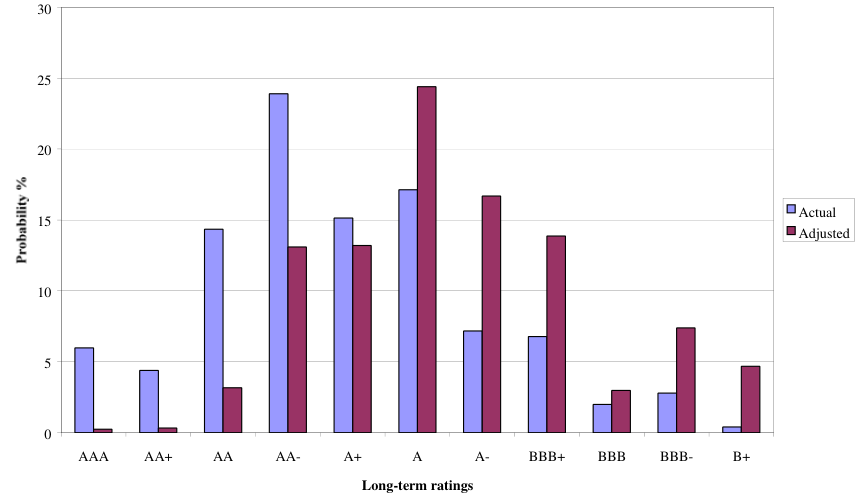
The results of these calculations appear in Chart 1. The chart shows the actual distribution of the ratings for the G10 banks rated by FitchIBCA at end-1998 and the distribution of the estimated ratings assuming very low support. The median actual rating is AA- but falls to A after the adjustment to remove the effect of support. An A rating (if FitchIBCA deliver a similar default likelihood to S&P) would be equivalent to a solvency standard of 99.96%.

To conclude, the evidence provided by the ratings that banks obtained from ratings agencies (adjusted for likely support) suggests that banks are targeting confidence levels of around 99.96%, which is considerably greater than the solvency standard implicit in the Basel Accord (ranging from 99.9% to 99%).(18)

4.2 Evidence from banks’ Tier 1 holdings

Another way to estimate a bank’s internal target solvency standard is to use the information from banks’ own holdings of Tier 1 capital. Typically, G10 banks hold Tier 1 capital that is substantially greater than the regulatory minimum. Indeed, the median Tier 1 ratio for the sample of 251 banks in our Bankscope sample is 7% compared with the Basel minimum of 4%. A credit risk model can be used to estimate the banks’ solvency standards given the amount of Tier 1 capital they hold, as long as there is information on the quality distribution of their portfolios.

Unfortunately, relatively few banks publish information on the distribution of their loans across ratings categories and even fewer do so for rating categories that correspond with those of the international rating agencies.

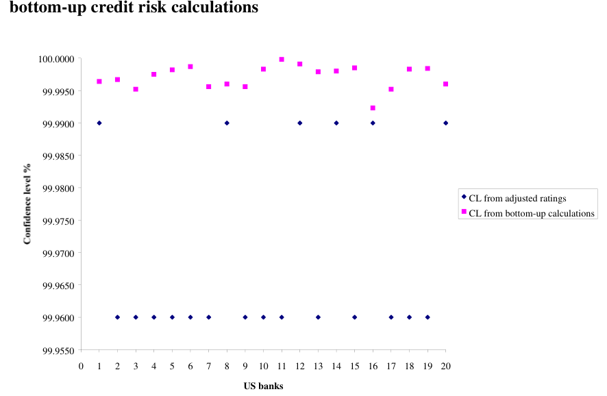
We therefore restrict attention to 20 large US banks within our sample of 251 G10 banks and compare the solvency standards implied by their agency ratings (adjusted for support) with the solvency standard implied by a CreditMetrics calculation, assuming their loan book corresponded to that of the high quality US bank described in a previous section.(19) Given that all the banks in the sample hold capital in excess of the minimum, the implied solvency standards calculated in this way are significantly higher than those shown in Section 2 for the high quality US book, being in the range 99.9964% to 99.9984% with a median solvency standard of 99.9977%.

Chart 2 compares the solvency standards for each bank calculated using the bank’s actual Tier 1 capital with the standard estimated for the bank from the calculated ‘long-term’ support-free ratings. The solvency levels imputed from the support-free ratings are lower than those calculated using the CreditMetrics approach and the banks’ own holdings of Tier 1. The solvency standard calculated for these banks from the rating is between 99.96% and 99.99%. This could be partly explained by the fact that CreditMetrics-style calculations may overestimate the confidence level and that rating agencies take into account as well, risks other than credit risk: such as market, liquidity and operational risks.(20)

(18) The first of these confidence levels corresponds to a AAA or AA grade, while the range from 99.9% to 99% corresponds to A to BBB ratings.

(19) The banks involved tend to be high credit quality so this is more appropriate than using the average-quality book employed elsewhere in earlier sections.

(20) That said, rating agencies would also take into account risk from retail assets, which tend to have a lower contribution to portfolio credit risk than the corporate assets considered here.

Table H summarises the results of the calculations of the target solvency levels of the individual banks compared with the solvency standard delivered by the current Basel Accord. We find that banks’ target solvency standards are considerably more conservative than the standard delivered by current minimum capital requirements even for high quality banks.

Table H: Solvency standards— current Accord versus banks’ own targets

Confidence interval Equivalent rating Current Basel Accord

Chart 1Copy link

Chart 2Copy link

5 Evidence on the effect of the solvency standard on market access

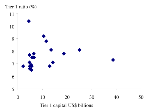
Why do banks maintain capital levels in excess of those required by the current regulatory minimum? A possible explanation might be that some countries impose higher regulatory capital requirements than the basic Basel Accord minimum. However, even in the United States where, under FIDICIA,(21) the authorities set perhaps the highest across the board requirements of any country for banks that want to be in the well-capitalised category,(22) the large banks maintain substantial excess capital. Most of the large US banks considered in the previous section have Tier 1 ratios (as per year end 1999) significantly in excess of the 6% minimum set for the well-capitalised banks (see below).

A second possible explanation is that banks maintain a buffer above the regulatory minimum level of capital so as to reduce the likelihood that a shock will lead them to breach their regulatory capital requirement in a costly fashion. (See eg, Milne (2001) who argues this.) If this were true, a reduction in the Basel standard or in any local requirements would permit banks to target a lower confidence level. A third possible explanation is that banks maintain confidence levels higher than the regulatory minimum in order to limit their funding costs and obtain access to important unsecured credit markets. Interbank rates and counterparty limits are highly sensitive to rating.(23)

Distinguishing the second from the third explanations empirically is difficult. In this section, we content ourselves with documenting the third explanation by examining the association between swap volumes and credit quality. The Bank of England has quarterly data on the gross mark to market swap liabilities of individual

____________________________________________________________________ __________

(21) Under the Federal Deposit Insurance Corporation Improvement Act of 1991 (FIDICIA), for a bank to meet the well-capitalised requirements it must have a total risk assets ratio of 10% and a Tier 1 ratio of 6%.

(22) For a group to become a financial holding company, all of the depositary institutions in the group must be well capitalised. Well-capitalised banks with the best CAMEL ratings pay no deposit insurance premium.

(23) Highly rated banks are able to borrow at LIBOR minus.

banks operating in the London market to the rest of the market. As limits vis-à-vis particular counterparties are set by many banks on the gross exposure as well as, or instead of, the net exposure, these data can be used to explore the sensitivity of access to the swap market to a bank’s rating. The last BIS survey of Foreign Exchange and Derivatives Market Activity (1998) showed that turnover in OTC derivatives in the London market in April 1998 amounted to $591 billion a day, twice the volume of any of the other national markets. Given the importance of the market, all large players have a sizable presence.

The data we employ here consist of information on the interest rate and foreign exchange swap liabilities (at market value) of individual banks (to the rest of the market) for the seven quarters, 1998 Q2-1999 Q4. At the end of 1999, our sample includes 48 banks (although the number of banks was slightly different in other quarters). Of the 48 banks, 39 had FitchIBCA ratings, all of which were A- or above except for two banks which, for at least one of the quarters, had ratings in the BBB to BBB+ range. Both of these relatively low credit quality banks held much smaller swap liabilities than average. The average level of quarterly swap liabilities across all banks was £5.8 billion and the median level was £0.9 billion.(24)

To investigate the association between credit quality and swap market volumes, individual banks’ swap liabilities, pooled across all seven quarters, were regressed against: (i) long-term FitchIBCA ratings (mapped into a numerical scale employed by Bloomberg to place ratings of different rating agencies on an equivalent basis)(25) and (ii) bank size, as measured by the log of total assets.(26) More formally, if yit equals the swap liabilities of bank i in quarter t, and all seven time series observations are pooled in a (column) vector yi, we can write

yi = X iβ+εi (4)

where β is a vector of parameters and the X i vector contains a constant, the bank’s

rating and the size of its assets. The coefficient on the rating variable can then be interpreted as the sensitivity of banks’ swap liabilities to credit quality after one has controlled for differences across bank size and for any fixed effect of time. The panel can be estimated using least squares with White-adjusted standard errors, to allow for the fact that the cross-sectional variance is probably not constant.

The results of the estimation are given in the second column of Table I below. Standard errors are reported in brackets and suggest that the coefficient of credit quality in both regressions is significant at the 1% level. The adjusted R-square is 19%, which is reasonable for cross-sectional data of this kind. The coefficient magnitudes suggest that a difference in a rating of one notch (eg from A to A+) is associated with a difference in the swap liabilities of roughly £2.2 billion.

____________________________________________________________________ __________

(24) Our sample is fairly homogeneous since it comprises only major investment banks or large commercial banks.

(25) The mapping employed by Bloomberg is: AAA (27), AA+ (25), AA (24), AA- (23), A+ (22), A (21), A- (20), BBB+ (19), BBB (18).

(26) We also employed time dummies to check whether higher liabilities were associated with particular quarters. The coefficients associated with the dummies were insignificant and the coefficients of the other two variables were almost identical to those reported in Table I.

Typically, rating agencies take into account the total size of a bank when assigning a rating. This raises the possibility that the sensitivity of swap activity to ratings reflects near co-linearity of the regressors for total assets and ratings. The typical symptoms of near co-linearity are high standard errors, low R-square statistics and sensitivity to the removal of observations (eg Greene 1990). The first two symptoms are not apparent in our results. We checked for the third by rerunning the regression after having randomly removed 10% of the observations and found that the specification is robust.

Table I: Regression results of swap liabilities (£m)

Constant 55221 (10109)** Long term rating 2251 (380.2)** Log of total assets 759.5 (386.0) Number of observations 294 Adjusted R-square 19.5

This evidence suggests that a bank that wishes to deal in significant swap volumes (relative to the size of its balance sheet) would certainly have to maintain a high rating so that counterparty limits are high. Large banks that just want to use swaps to hedge their own interest rate and FX exposure might also need fairly large counterparty limits. For example, this would be necessary to enable large fixed-rate subordinated debt issues to be swapped into floating and hedge large variations in interest rate exposures in the banking book. One large bank with which we have had discussions indicates that swap trading to hedge its own positions can amount to around £20 billion a month.

The greater use of collateralisation in the market over the past two or three years makes it easier for lower-rated counterparties to have some access to the market but they would need to limit use of swaps because of the cost – keeping to passive hedging strategies, for example. Therefore if a bank’s rating declines below a certain threshold level, it will likely have to change its way of doing business by, for instance, match funding more of its book to reduce reliance on swaps for hedging and by collateralising its remaining swap exposures. Anecdotal evidence indicates that banks need to try to keep at least an A rating to retain a reasonable degree of flexibility.

The above findings are consistent with the results of several papers about US banks. Bhasin (1995) compares the external ratings of all US OTC derivative participants with those of the market at large. He finds that OTC derivative users are consistently and significantly more highly rated than other firms in general. He finds that some low-rated banks participate in the market but he does not look at the size of the exposures to them (which could be very small). Gunther and Siems

(1995) find a positive relationship between capitalisation and participation in the OTC derivatives market.

Chart 3Copy link

6 Conclusion

The purpose of internationally agreed minimum capital standards for significant banks is to limit the default probability of banks so as to maintain financial stability. An important policy choice for bank regulators is the level at which average regulatory capital levels should be set or alternatively what survival probabilities are acceptable for representative banks. This paper investigates the survival probabilities or solvency standards implied by current regulations and the ‘economic’ solvency standards implicit in banks’ own capital decisions.

Our study suggests that the current Basel Accord delivers a confidence level for large banks of around 99.9% (equivalent to the upper end of BBB) for banks with high-quality books, but a much lower standard of 99% (or BB) for banks with lower quality portfolios.

It has been suggested by some banks and banking associations that the new Accord should be set at a lower level than the current Accord. But a minimum capital level for a large bank must be set at a level at which the bank is still viable. If large banks generally have to target solvency standards that are much higher than those implicit in the current Accord, in order to have the flexibility to carry out the type of business in which they are engaged, this may indicate that the current level is already quite low.

In this article, we have examined two sources of information on banks’ target solvency levels, (i) the agency credit rating they achieve and (ii) the Tier 1 capital (equity and reserves) they choose to maintain. On (i), most banks have a rating above BBB – the median Moody’s, Standard and Poor’s and FitchIBCA ratings are A1, A+ and AA- respectively. But these ratings are boosted by assumptions made by the rating agencies regarding possible support in times of difficulty. Empirical analysis to strip out the effect of support indicates that the median FitchIBCA standalone long-term rating would be A, equivalent to a confidence level of 99.96%. This is higher than the solvency standard delivered by the current Basel Accord for high-quality banks.

On (ii), most banks certainly carry substantially more Tier 1 capital than required by the Basel Accord. Calculating the confidence level for the banks using their own Tier 1 capital (after making assumptions about credit quality) points to rather higher solvency levels than those that appear to underlie the ratings for individual banks. This may reflect the fact that the rating agencies take into account risks other than credit risk faced by the banks – for example operational risk.

On balance, the evidence suggests that banks large enough to have a rating, target a solvency standard that is significantly more conservative than that delivered by the current Basel Accord. An important issue is why the banks target these higher solvency standards. It is sometimes argued that it is to provide a buffer above the regulatory minimum to reduce the likelihood of a breach. Alternatively the banks might have to target the particular ratings they have in order to gain access to particular markets.

While it is difficult to distinguish these hypotheses empirically, in this study we at least document the market discipline hypothesis by examining the way in which banks’ solvency standards (as evidenced by their ratings) appear to influence their access to the swap market. We find that, below a rating of A-, swap liabilities become very small compared to the average. We interpret this as indicating that banks with ratings below this level have a much reduced access to the market. A bank moving from A to BBB would have to change its ways of doing business to limit the recourse to swaps because of cost and access issues.

Banking authorities probably need to take into account the likelihood that a reduction in the capital of a large bank could affect its market access, even when its capital exceeds the minimum set by the 1988 Basel Accord. This could possibly have an impact on the viability of even a large bank. This is perhaps a consideration that supervisory authorities should have in mind for the future when considering minimum capital requirements for the largest banks.

Appendix on the 1988 Basel Accord capital rules

The 1988 Basel Accord defined a bank’s risk weighted assets as a weighted sum of different assets held by the bank. A small number of risk weights (0, 10, 20, 50 and 100%) were employed. Exposures to OECD member sovereigns (and local currency exposures to other sovereigns) are risk-weighted at 0%. All exposures to banks located in OECD countries receive a 20% weighting. For claims on banks incorporated outside the OECD there is a 20% weight for under one year exposure and 100% for over one year. Zero weight apply to cash and gold bullion. 100% is the weighting applied to all claims on the non-bank sector, irrespective of the credit quality of the exposure. The only exception is residential mortgage exposures that are risk-weighted at 50%. Transactions that are fully collateralised by cash or by OECD government and bank securities attract the risk weight associated with these assets. There is also a simple way of treating off-balance-sheet items such as commitments.

The Accord defined Tier 1 capital to consist of shareholders’ equity capital plus published disclosed reserves, and Tier 2 capital to comprise undisclosed and revaluation reserves, general provisions up to 1.25% of total risk-weighted assets, hybrid and subordinated term debt. Goodwill and equity investment in certain unconsolidated subsidiaries were deducted from capital.

The Accord requires internationally active banks regulated in G10 countries to hold Tier 1 plus Tier 2 capital at least equivalent to 8% of their risk-weighted assets and to hold Tier 1 capital in excess of 4% of risk-weighted assets. The Accord was agreed in 1988, but transitional arrangements existed up until the end of 1992, at which time full observance was required.

References

Asarnow, E and Edwards, D (1996), ‘Measuring loss on defaulted bank loans: a 24-year study’, Journal of Commercial Lending, January, pages 11-23.

Bank for International Settlements (1998), Central bank survey of foreign exchange and derivatives market activity, Monetary and Economic Department.

Basel Committee on Banking Supervision (1999), ‘A new capital adequacy framework: consultative paper’, June.

Basel Committee on Banking Supervision (2001), ‘ The new Basel Accord: consultative package’, January.

Bhasin, V (1995), ‘On the credit risk of OTC derivative users’, Federal Reserve Board working paper 95-50, November.

Bucay, N and Rosen, D (2000), ‘Applying portfolio credit risk models to retail portfolios’, Algo Research Quarterly, Vol. 3, pages 45-73.

Cantor, R and Falkenstein, E (2001), ‘Testing for rating consistency in annual default rates’, Moodys Investors Service Global Credit Research, February.

Carey, M (2001), ‘A policymaker’s guide to choosing absolute capital requirements under an IRB approach’, Board of Governors of the Federal Reserve working paper.

Carty, L and Lieberman, D (1996), ‘Defaulted bank loan recoveries’, Moody’s Global Credit Research, Special Report.

Credit Suisse Financial Products (1997), CreditRisk+: a credit risk management framework, Technical manual.

FDIC (1998), Managing the crisis: the FDIC and RTC experience, Federal Deposit Insurance Corporation, August, Washington DC.

FitchIBCA (1998), Bank rating methodology, April.

Gordy, M (2000), ‘A comparative anatomy of credit risk models’, Journal of Banking and Finance, Vol. 24, pages 119-49.

Greene, W H (1990), Econometric analysis, Prentice Hall: 2nd edition.

Gunther, J W and Siems, T F (1995), ‘Who’s capitalising on derivatives’, Federal Reserve Bank of Dallas Financial Industry Studies, July, pages 1-8.

Hu, Y-T and Perraudin, W (2001), ‘Recoveries and defaults: correlation and Value-at-Risk’, Birkbeck College, mimeo.

Hu, Y-T, Jackson, P, Perraudin, W and Saporta, V (2001), ‘The impact of support on bank ratings’, Bank of England, mimeo.

International Monetary Fund (1998), ‘Financial crises: characteristics and indicators of vulnerability’, in World Economic Outlook (Chapter 4), May.

JP Morgan (1997), CreditMetrics –Technical Document, JP Morgan New York.

Kiesel, R, Perraudin, W and Taylor, A (2001), ‘The structure of credit risk’, Bank of England Working Paper no 131.

Milne, A (2001), ‘Bank capital regulation as an incentive mechanism: implications for portfolio choice’, City University Business School, mimeo.

Nickell, P, and Perraudin, W (2001), ‘How much bank capital is needed to maintain financial stability?’, forthcoming Bank of England working paper.

Nickell, P, Perraudin, W and Varotto, S (2000), ‘Stability of ratings transitions’, Journal of Banking and Finance, Vol. 24, pages 203-27.

Nickell, P, Perraudin, W and Varotto, S (2001), ‘Ratings versus equity-based credit risk modelling: an empirical analysis’, Bank of England Working Paper no.132.

Ronn, E and Verma, A (1989), ‘Risk-based capital adequacy standards for a sample of 43 banks’, Journal of Banking and Finance, Vol. 13, pages 21-29.

Varotto, S (2000), ‘Credit risk diversification and bank capital’, Birkbeck College, mimeo.

Notes

(6) In preparing these ratings distributions, Federal Reserve staff mapped internal bank ratings to agency ratings grades. (13) In mapping the confidence levels calculated under the three-year default basis assumption into S&P ratings, one needs to employ three-year cumulative, rather than the one-year S&P default rates. S&P report average three-year cumulative rates of 0.03, 0.09, 0.19, 0.79, 5.35% corresponding to ratings AAA, AA, A, BBB and BB respectively. Banks with high quality books 99.90 BBB+ Banks with average quality books 99.00 BB-, BB+ Bank’s own target solvency standards Evidence from long term ratings (median) 99.99 AA- Evidence from long term ratings adjusted to remove support 99.96 A (median) 99.9977 AA Evidence from banks’ own Tier 1 holdings— US banks using the high quality distribution (median) ** Significant at 1% level.