

For stress testing and strategy formulation, it is important for asset managers to forecast their Assets under Management (AUM) accurately. This paper develops statistical methods for forecasting AUM and applies them to data for 2,494 UK, French, German and Italian-domiciled funds. The results allow one to project forward AUM under different assumptions about market conditions and in a way that is customised for the age, size and fund flow and return histories of the funds in question.
Executive Summary
For stress testing and strategy formulation, it is important for asset managers to forecast their Assets under Management (AUM) accurately. This paper develops statistical methods for forecasting AUM and applies them to data for 2,494 UK, French, German and Italian-domiciled funds. The results allow one to project forward AUM under different assumptions about market conditions and in a way that is customised for the age, size and fund flow and return histories of the funds in question.
Building on an extensive academic literature, we employ an approach that splits the dynamics of AUM into the contributions of returns and of fund flow (defined as the change in AUM less the effects of returns). We use statistical methods to model these two components separately and then combine the models to generate forecasts of AUM itself.
The effects implied by our estimates are broadly intuitive (in a qualitative sense) for the four domiciles of funds that we analyse. Lagged fund flow and lagged returns imply higher (percentage) growth as does being a young or a small fund. However, the (quantitative) sensitivities of fund flow to different effects and, in particular to lagged returns and lagged fund flow, are much greater for UK funds than for those from other domiciles we consider. Italian funds are least sensitive in this regard. We, also, find very pronounced non-linearities in the relations between fund flow and several of its key determinants.
1. Introduction
The profitability of investment firms depends on their ability to attract and retain Assets under Management (AUM). Forecasting AUM for a given fund or set of funds is, therefore, key to financial planning for such firms. Forecasting may be performed either unconditionally or conditional on particular scenarios. In the latter case, AUM forecasts may be employed in stress testing exercises.
In this note, we develop techniques for forecasting a fund’s AUM. The approach we take consists of forecasting fund flow (the new money invested in a fund in a given period) and fund returns from which one may deduce the future path of AUM. For fund i at time t, the fund flow is defined by equation (1).
AUMi,t−AUMi,t−1∙(1+ri,t) (1) Flowi,t = AUMi,t−1
Here, AUMi,t is the AUM of the fund at date t, and ri,t is the net return on the fund over the period t−1 to t. Clearly, rearranging equation (1), one may express AUMi,t in terms of Flowi,t , ri,t and AUMi,t−1. Hence, given a set of forecasts of Flowi,t , ri,t and AUMi,t−1 one may recursively infer forecasts for future AUM.
We forecast fund flow as autoregressive processes with a series of forcing variables. These include lagged returns, size, age and some lagged market variables: equity returns and interest rate changes. In stress testing exercises, time paths for these market variables will typically be specified which is why we condition on these.
Based on univariate regressions, we present evidence that the dependence of fund flow on the independent variables is non-linear. To cope with this feature of the data, we employ piecewise regressions. This boosts the explanatory power of the forecasting models we formulate according to degrees of freedom-adjusted R-squared goodness of fit measures.
Last, to analyse the effectiveness of the piecewise regression models in forecasting, we examine what they imply for the impact on AUM of different sets of explanatory variables. To this effect, we perform a series of impact response calculations in which we project AUM for funds grouped into quintile subsets of the funds (with a particular domicile) where the quintiles are based on the values of a given explanatory variable. This yields an estimate of the average impact on AUM forecasts of being in the highest (versus the lowest) lagged fund flow or fund return quintiles.
The results suggest that lagged fund flow is quantitatively the most important factor for subsequent AUM growth although lagged return, size and age also have significant effects. The magnitude of effects is greatest for UK domiciled funds followed by French and then German funds. Overall, Italian funds exhibit the smallest impact effects.
The note is organised as follows. Section 2 surveys the academic literature on the determinants of fund flows. Section 3 describes the fund data used in the analysis, and the regression model used to predict fund flow. Section 4 presents the results of the regressions and an impact response analysis. Section 5 concludes.
2. Determinants of fund flow
There is a substantial academic literature on the determinants of fund flow. Past studies mostly focus on the U.S. fund market. This is larger and more developed than the European market although the European market has grown rapidly in recent years.
Chevalier and Ellison (1997) and Sirri and Tufano (1998) show that past returns influence future fund flows, and moreover investors in high performing funds are much more sensitive to past returns than investors in low performing funds. Chevalier and Ellison (1997) then show that the relationship between past returns and fund flows can provide fund companies with incentives to adjust the riskiness of their portfolios to attempt to avoid underperforming the market and so attract investors. They provide empirical evidence that the behaviour of fund companies is consistent with these incentives.
Despite the returns-flow relationship, there is mixed evidence for the persistence of returns that would justify investor behaviour. Carhart (1997) and Hendricks, Patel, and Zeckhauser (1993) find strong evidence for persistence among poor-performing funds, though less evidence for persistence among high-performers. Grinblatt and Titman (1992), Goetzmann and Ibbotson (1994) and Daniel et al. (1997) find evidence for persistence among high-performers, though Bollen and Busse (2004) find that this only holds in the shortterm.
Berk and Green (2004) offer an explanation of the relationship between past returns and future flows which is consistent with little persistence among high performers. In their model, high returns serve as a signal of managerial ability, however, due to decreasing returns to scale, the flow of funds in response to this signal make the high returns unsustainable.
As well as past returns, a variety of performance and risk metrics have been examined as possible determinants of fund flows. These include advertising and marketing expenses (Jain and Wu (2000) and Huang, Wei and Yan (2007)) and Morningstar ratings (Nanda, Wang and Zheng (2004), Huang, Wei and Yan (2007) and Del Guercio and Tkac (2008)).
Finally, Clifford et al. (2013) examine the impact of risk on fund flows. The authors study inflows and outflows separately and find that, while investors are indifferent to the systemic risk of a fund, higher levels of idiosyncratic risk correspond to larger inflows as well as outflows. This unintuitive result is explained by investors following high past returns, as funds achieving these high returns will tend to display higher levels of idiosyncratic risk.
3. Data and methodology
3.1 Data
The data used in this study was obtained from Bloomberg which provides monthly historical total net assets and returns data for a large number of funds. Liquidated funds remain in the dataset so the results should be free from survivorship bias. In this note, we study the behaviour of 2494 UK, French, German and Italian funds. The sample period extends from January 2006 to July 2016. Bond funds were removed from the sample to be consistent with literature examining U.S. funds.
The Bloomberg AUM data suffer from various problems. Yearly or quarterly data is sometimes substituted for monthly data, with missing periods filled with duplicate values. There are occasional extreme spikes, which mostly appear to be the result of data entry errors. As the size of the dataset made the task of manually checking each possible error infeasible, data points that were judged to have a high likelihood of being erroneous were removed automatically. Single month gaps in AUM were filled using linear interpolation. Both quarterly returns and the calculated fund flows are winsorised at the 0.5% level. For fund flows this is particularly important as mergers and other restructuring of funds by the parent firm can lead to large outliers that are unrelated to investor behaviour.
Table 1 provides information on the funds employed in the study broken down by domicile. Most of the funds in the sample are French, with just over half the remainder being domiciled in the U.K. While French and German funds account for most of the AUM at the start of the sample period, by the end of the sample period U.K. funds account for over 50% of the total AUM.
Note: This table presents information on the funds in the four domiciles considered. The number of funds is shown broken down by the regional focus of the fund, as assigned by Bloomberg. The evolution of the total AUM is shown with snapshots at the end of Q1 in each of 2006, 2011 and 2016. The lower half of the table shows the lower, middle and upper quartiles of the distributions of quarterly returns and fund flow for the entire sample.
UK based funds yield higher returns but exhibit more cross sectional variation. Non-UK funds are more prone to negative than positive fund flow whereas UK funds appear more balanced in this respect.
| Regional focus | France | Germany | Italy | U.K. | Total |
|---|---|---|---|---|---|
| Europe | 795 | 140 | 81 | 86 | 1102 |
| Global | 420 | 190 | 128 | 387 | 1125 |
| U.K. | 0 | 0 | 0 | 267 | 267 |
| All funds | 1215 | 330 | 209 | 740 | 2494 |
| Assets under | management | (EUR billions) | |||
| Year | France | Germany | Italy | U.K. | Total |
| 2006 Q1 | 110.59 | 94.10 | 17.89 | 59.06 | 281.64 |
| 2011 Q1 | 174.58 | 76.19 | 24.80 | 235.85 | 511.43 |
| 2016 Q1 | 186.22 | 94.64 | 20.51 | 414.25 | 715.63 |
| Quarterly returns | (%) | ||||
| Quartile | France | Germany | Italy | U.K. | All |
| Lower | -2.33 | -2.29 | -3.44 | -1.97 | -2.27 |
| Median | 1.84 | 1.99 | 1.30 | 2.65 | 2.03 |
| Upper | 5.53 | 5.65 | 4.78 | 6.28 | 5.73 |
| Quarterly fund flow | (%) | ||||
| Quartile | France | Germany | Italy | U.K. | All |
| Lower | -3.52 | -4.15 | -6.65 | -4.83 | -4.07 |
| Median | -0.50 | -1.18 | -1.78 | 0.22 | -0.58 |
| Upper | 2.35 | 1.34 | 3.40 | 4.76 | 2.93 |
3.2 Regression specification
To estimate fund flows, we employ an autoregressive model. To capture the well documented performance-flow relationship, the quarterly and annual (twelve month) returns as measured in the previous quarter are included as regressors.
The size and age of a fund can have a noticeable effect on inflows and outflows. In particular, smaller, younger funds are more likely to see rapid growth than larger, older funds. This is captured in the model by including the logarithm of the fund AUM in EUR millions and the inverse of the age of the fund in months as regressors.
Lastly, three time-series variables capturing the changes in market conditions are included in the regressions:
1. Quarterly difference in log equity index,
2. Quarterly difference in 3m treasury bill rates,
3. Quarterly difference in 10y government benchmark bond yield. UK treasury bills and bonds are used for the UK, and Euro area treasury bills and bonds for France, Germany and Italy. For the UK the FTSE All-Share index is used, while the Euro Stoxx index is used for the remaining domiciles.
Note that a primary purpose of this study is to provide predictive models of AUM that can be used in stress testing exercises. Stress scenarios typically involve specifying time paths for market variables including interest rates and equity indices and then deducing, conditional on those time paths, the likely evolution of AUM. The fund’s profitability and the evolution of its earnings statement and balance sheet may then be inferred by imposing on top of the AUM forecasts, hypotheses about fees, costs etc. The objective of facilitating such an analysis is what motivates the regression model as just described.
The basic regression model corresponding to the model described above is specified by the equation:
Flowi,t = α+ ∑τ=1 βFlow,τ ∙Flowi,t−τ +βReturn ∙Returni,t−1 + βAnnualReturn ∙AnnualReturni,t−1 −1 (2) +βAUM ∙log(AUMi,t−1) + βAge ∙(Agei,t−1) +βEquity ∙∆log(Equityt−1) + β3mRate ∙∆3mRatet−1 + β10yRate ∙∆10yRatet−1 +εi,t
It is highly likely that the relationship between fund flow and the regressors shown in equation (2) is actually non-linear. To capture non-linearity, we also employ a more complex piecewise regression model. Let X be an exogenous variable, and let b[1] < ⋯< bn be a sequence of breakpoints for X. Then, for 0 ≤j≤n we define in equation (3) a set of variables X(j):
bj X≤bj X X(j) = { bi < X< bj+1 (3)
bj+1 X≥bj+1
In the segmented fund flow model, the same fundamental variables are used, but two breakpoints are allowed for each lagged flow variable, and one breakpoint for the lagged quarterly and annual returns, and the log AUM. This is summarised by the equation:
(j) ∑ Flowi,t = α+ ∑τ=1 j=0 βFlow,τ,j ∙Flowi,t−τ
(j) (j) 1 1 + ∑j=0 βReturn,j ∙Returni,t−1 + ∑j=0 βAnnualReturn,j ∙AnnualReturni,t−1 −1 1 (4) + ∑j=0 βAUM,j ∙log (AUMi,t−1(j) ) + βAge ∙(Agei,t−1)
+βEquity ∙∆log(Equityt−1) + β3mRate ∙∆3mRatet−1 + β10yRate ∙∆10yRatet−1 +εi,t
Different breakpoints are used for each domicile. The breakpoints used are specified in Tables 2 and 3. All standard errors are calculated with allowance for two-way clustering on time and fund. This has the advantage over the Fama-MacBeth regression procedure proposed in Fama and MacBeth (1973) that it corrects for fund effects as well as time effects. Petersen (2009) presents a comprehensive comparison of the different approaches.
4. Results
4.1 Univariate relations to fund flow
Appropriate breakpoints for each exogenous variable were found by univariate plots against fund flow and by nonlinear regression analysis. Figure 1 displays plots of the quarterly fund flow against five different explanatory variables: (i) the one-period lagged quarterly fund flow, (ii) the quarterly return on the fund, (iii) the annual return on the fund, (iv) the inverse of the age of the fund in months, and (v) the natural logarithm of AUM.
For each plot, the explanatory variable, considered over the entire sample period and for each fund in the specified domicile, is divided into 20 quantiles. The average value of the explanatory variable in the quantile is then plotted against the average value of the fund flow for those observations.
For the U.K., France and Germany the plots of fund flow versus lagged fund flow show similar features. Higher past flows correspond to higher contemporaneous flows and this effect is most marked when the past flow is in the range of −5% to around 20%. The relationship is also apparently non-linear for Italian funds.
The relationship between past returns and fund flows is similarly positive. Here, a non-linearity may be observed around 0% for U.K, France and Germany, with higher, positive returns being more strongly correlated with higher fund flows. This is observable for both lagged quarterly and lagged annual returns, though Italian funds again behave differently.
The last two rows of Figure 1 show plots of the fund flow versus the inverse of the age of the fund in months and the log AUM in EUR millions. In all four domiciles smaller, younger funds seem to attract higher fund flows. After taking logarithms there is still an apparent non-linearity in the relationship between fund flow and lagged AUM.
The breakpoints chosen are shown in Table 3. The same breakpoints are used for the one, two and three period lagged fund flow: one breakpoint at −5% and another at 15 −25% dependent on country. A breakpoint at 0% is used both for lagged quarterly returns and for lagged annual returns. For the log lagged AUM, a breakpoint between 0.5 −1.5% is used, varying by country. No breakpoint is used for the inverse age of the fund.
Coeff. t-stat. Coeff. t-stat. Coeff. t-stat. Coeff. t-stat.
Constant 0.018 3.055 0.018 5.462 -0.001 -0.153 0.048 3.784
Flow lag 1 0.218 10.850 0.179 15.390 0.122 5.199 0.083 3.143
Flow lag 2 0.136 8.015 0.044 3.740 0.084 4.228 0.085 3.177
Flow lag 3 0.073 4.643 0.037 4.463 0.044 3.248 0.044 2.676
Return lag 1 0.161 6.064 0.203 9.317 0.103 3.035 0.761 12.287
Annual return lag 1 0.101 10.129 0.023 3.547 0.043 3.845 -0.120 -6.507
Log AUM lag 1 -0.016 -7.356 -0.017 -11.379 -0.008 -3.476 -0.025 -4.578
Inverse age 0.896 5.698 0.955 8.427 0.524 2.452 0.134 0.290
Equity lag 1 -0.028 -0.900 -0.065 -3.761 -0.015 -0.543 -0.238 -6.297
3m rate lag 1 -0.020 -3.137 -0.033 -10.504 -0.043 -9.594 0.039 5.996
10y rate lag 1 0.006 1.483 0.021 5.946 0.017 2.940 0.037 3.639
Number of observations 11,626 35,198 8,946 3,563
R-squared 0.170 0.068 0.052 0.144
Adjusted R-squared 0.170 0.068 0.051 0.141
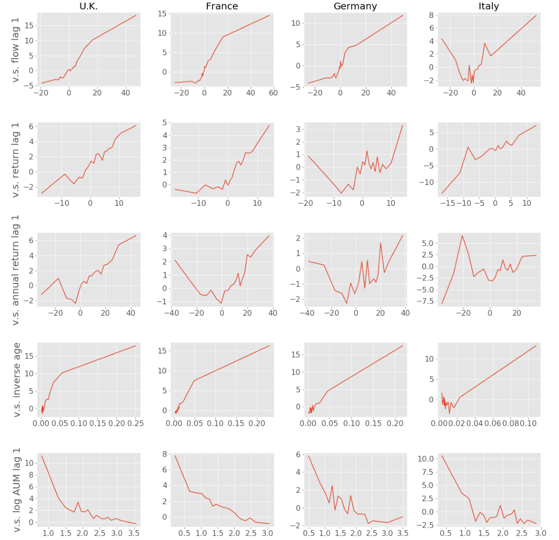
Note: This figure shows univariate relations between fund flow and five explanatory variables for the four fund domiciles in the sample. Here, age is measured in months and AUM in EUR millions. For each plot, the explanatory variable is divided into 20 quantiles and the mean of the explanatory variable in each quantile is plotted against the mean flow in that quantile.
| Breakpt. | Coeff. | t-stat. | Breakpt. | Coeff. | t-stat. | Breakpt. | Coeff. | t-stat. | Breakpt. | Coeff. | t-stat. | ||
|---|---|---|---|---|---|---|---|---|---|---|---|---|---|
| Constant | 0.085 | 3.525 | 0.015 | 1.079 | 0.057 | 1.954 | 0.113 | 3.042 | |||||
| Flow lag 1 | piece 1 | -0.050 | 0.067 | 1.406 | -0.050 | 0.059 | 2.177 | -0.050 | 0.106 | 1.668 | -0.050 | 0.084 | 1.044 |
| Flow lag 1 | piece 2 | 0.250 | 0.427 | 16.888 | 0.150 | 0.434 | 17.545 | 0.250 | 0.360 | 7.598 | 0.200 | 0.267 | 5.619 |
| Flow lag 1 | piece 3 | 0.023 | 0.594 | 0.093 | 4.702 | -0.071 | -1.951 | -0.043 | -1.012 | ||||
| Flow lag 2 | piece 1 | -0.050 | 0.088 | 1.759 | -0.050 | -0.040 | -1.364 | -0.050 | 0.058 | 1.465 | -0.050 | 0.030 | 0.341 |
| Flow lag 2 | piece 2 | 0.250 | 0.291 | 12.429 | 0.150 | 0.168 | 6.773 | 0.250 | 0.154 | 4.208 | 0.200 | 0.170 | 3.194 |
| Flow lag 2 | piece 3 | -0.032 | -1.027 | -0.004 | -0.252 | 0.001 | 0.018 | 0.043 | 0.960 | ||||
| Flow lag 3 | piece 1 | -0.050 | 0.012 | 0.290 | -0.050 | -0.057 | -1.880 | -0.050 | 0.087 | 2.332 | -0.050 | 0.011 | 0.215 |
| Flow lag 3 | piece 2 | 0.250 | 0.047 | 2.088 | 0.150 | 0.040 | 1.942 | 0.250 | 0.082 | 2.691 | 0.200 | 0.030 | 0.645 |
| Flow lag 3 | piece 3 | 0.042 | 1.486 | 0.036 | 2.876 | -0.025 | -0.995 | 0.060 | 2.465 | ||||
| Return lag 1 | piece 1 | 0.000 | 0.113 | 2.221 | 0.000 | 0.146 | 4.713 | 0.000 | 0.051 | 1.047 | 0.000 | 0.782 | 9.104 |
| Return lag 1 | piece 2 | 0.231 | 6.913 | 0.211 | 6.675 | 0.098 | 1.810 | 0.802 | 7.933 | ||||
| Annual return | lag 1 piece 1 | 0.000 | 0.063 | 2.129 | 0.000 | -0.053 | -3.494 | 0.000 | 0.043 | 1.962 | 0.000 | -0.172 | -3.818 |
| Annual return | lag 1 piece 2 | 0.089 | 7.079 | 0.054 | 5.157 | 0.038 | 2.143 | -0.110 | -3.772 | ||||
| Log AUM lag | 1 piece 1 | 1.500 | -0.057 | -3.588 | 0.500 | -0.065 | -2.307 | 1.000 | -0.018 | -0.669 | 1.000 | -0.086 | -2.355 |
| Log AUM lag | 1 piece 2 | -0.012 | -5.818 | -0.014 | -11.056 | -0.008 | -3.745 | -0.018 | -3.592 | ||||
| Inverse age | 0.636 | 4.149 | 0.770 | 6.943 | 0.346 | 1.709 | -0.282 | -0.612 | |||||
| Equity lag 1 | -0.044 | -1.375 | -0.056 | -3.259 | -0.008 | -0.278 | -0.298 | -7.712 | |||||
| 3m rate lag1 | -0.018 | -2.357 | -0.017 | -3.856 | -0.040 | -7.154 | 0.053 | 4.739 | |||||
| 10y rate lag1 | 0.007 | 1.663 | 0.014 | 3.776 | 0.016 | 2.724 | 0.039 | 3.906 | |||||
| Number of | observations | 11,626 | 35,198 | 8,946 | 3,563 | ||||||||
| R-squared | 0.203 | 0.082 | 0.072 | 0.158 | |||||||||
| Adjusted | R-squared | 0.202 | 0.081 | 0.070 | 0.154 |
Note: This table shows regression results for each of the four fund domiciles included in the sample. The dependent variable is the contemporaneous quarterly fund flow. Lagged quarterly fund flows, lagged quarterly and annual returns, lagged log assets under management (EUR millions) and inverse age (months) are included as explanatory variables, with breakpoints indicated in a third column for each domicile. These breakpoints are domicile dependent, and are based in part on the univariate relations shown in Figure 1. Three macroeconomic variables are also included as explanatory variables: these are quarterly changes in the log of an equity index, in 3-month rates, and in 10-year rates.
4.2 Regression results
Regression results are presented in Tables 2 and 3. Table 2 shows the results of fund flow regressions for each domicile with no breakpoints being used, while Table 3 shows the results with breakpoints.
For all domiciles there is a consistently positive relationship between past and future fund flows. This is most pronounced for the U.K. and France, and least pronounced for Italy, both in the simple and the piecewise regressions. This relationship generally becomes weaker as the number of lags becomes greater. When using the piecewise regression framework it can be observed that the positive relationship is much stronger when the previous flow is in the mid-range, and outside of this range coefficients are inconsistent and the t-statistics become more negligible. This corresponds with the plots shown in Figure 1.
There is also a clear positive correspondence between high past returns and high flows into the fund. This relationship appears slightly less straightforward for Italian funds than for funds in the other domiciles, with lagged quarterly returns having a much higher impact on fund flows, but with lagged annual returns having a negative impact.
Across all four domiciles there is a consistent pattern of smaller, younger funds attracting more new money than older, larger funds. This aligns with the results of most studies of U.S. funds. Again, Italian funds behave slightly differently in this respect, with a much less noticeable difference in flows to older and younger funds. The relationship between log AUM and fund flow is most pronounced for smaller funds, confirming the plots shown in Figure 1.
4.3 Forecasting AUM and impact effects
To grasp the materiality of these piecewise regressions for understanding the likely future AUM of a fund, we examine the impact effect of changes in the explanatory variables. We calculate the impact effects for all the fund and time period observations[2] corresponding to a given domicile and then present averages.
The impact effects are calculated by dividing the observations for a particular domicile into 5 equal sized subsets based on the magnitude of a given variable of interest. For each subset, we average the variable of interest within the subset and average other independent variables in the regression across the whole sample period. We then project forward equation (4) assuming no shocks and that macroeconomic variables equal their sample averages.
Impact effects of this sort are calculated for four variables:
1. The 0-2 period lagged quarterly fund flow
2. The quarterly return on the fund
3. The inverse of the fund age in months, as of the next quarter
4. The logarithm of the AUM (EUR millions)
Note that, in the case of the lagged quarterly fund flow, the fund flows in different lagged periods are averaged. The variables (or averages of variables) are then separated into quintile subsets and a mean value is calculated for each quintile subset. For variables other than the variable of interest, a mean over the whole sample is calculated. The exception to this is the annual return: this is not calculated directly, rather the 1-3 period lagged quarterly return are averaged over the sample, and these are used in conjunction with the contemporaneous quarterly return to calculate the annual return. This enables the proper simulation forwards of the annual return variable.
This approach produces a set of five synthetic fund observations, differing only in the variables of interest, or, in case of the quarterly return on the fund, also in the lagged annual return. Equation (4) is then used to calculate the value of Flowi,t+1, where i= 1, ⋯,5 now denotes the quintile of the set of variables being studied rather than a specific fund. The coefficients used are taken from the regression results in Table 3, and changes in the macroeconomic variables and the Gaussian noise εi,t+1 are set to zero.
Taking Returni,t+1 to be the mean quarterly return over the entire sample also yields AUMi,t+1, using equation
(1) and the predicted value of Flowi,t+1. Once the value of Returni,t+1 is set, AnnualReturni,t+1 may also be calculated from the quarterly returns. In this manner the regression variables may be simulated forward period by period, with Returni,t+1 = ⋯= Returni,t+τ being fixed as the mean return, and εi,t+1 = ⋯= εi,t+τ = 0. This yields five AUM time paths, one for each quintile of the set of variables being considered. Finally, to make the results comparable, these AUM time paths are rescaled so that the initial AUM in each path is equal to unity.
The results reveal rather directly the economic materiality of the regression estimates. Figure 2 shows the result of these simulations for each domicile, and each set of variables. The top row of plots show forecast time paths for AUM corresponding to each of five quintile averages where the quintiles are based on the lagged 3 month fund flows. The individual plots are specific to each domicile considered.
The time paths in this first row exhibit consistent qualitative patterns. Funds in the quintile associated with the highest lagged fund flow generate high AUM growth (see the yellow line) while those with the lowest lagged fund flow imply the lowest AUM growth (see the red line). For all domiciles, funds that are in the highest lagged fund flow quintile enjoy exceptional subsequent growth. The lines corresponding to the other quintiles averages are somewhat closer to each other. While qualitatively similar, the first row plots in Figure 2, however, suggest some quantitative variation across domiciles in that the magnitude of lagged fund flow effects is much greater for the UK. At the six-year horizon of the forecasts, being in the highest UK quintile implies almost 70% greater growth compared to those in the middle quintile. The corresponding figures for French, German and Italian funds is 30%, 25% and 12%.
The second row of plots in Figure 2 exhibit the effects of being in different quintiles on a 1-quarter lagged return. Yellow lines correspond to forecasts for high lagged return funds whereas red lines represent projections for low lagged return funds. The forecast AUM time paths resemble each other for the different domiciles except for the Italian projections which exhibit greater mean reversion. The magnitudes of effects again vary considerably with UK funds varying from plus 20% to minus 10% for the highest and lowest lagged return quintiles, respectively. For France the figures are plus 5% and minus 6%, while for Germany and Italy they are, respectively, plus 4% and minus 6% and plus 3% and minus 4%. As for lagged fund flow, lagged return effects are much larger for UK funds, with French funds being the second most affected.
The third row of plots in Figure 2 shows how AUM growth is affected by inverse age. One might expect to see young funds growing more rapidly than old and this is the case for UK, French and German funds. The Italian data suggest an anomalous finding that young funds grow least rapidly. Italian funds overall are contracting in size and it may be a feature of our sample that the Italian fund management industry was affected by the crisis making growth difficult for young funds. The magnitudes of age effects are again greatest for UK funds, followed by French and then German.
The fourth row in Figure 2 shows size effects. All four domiciles exhibit similar qualitative patterns in that small funds tend to grow more and large funds show a tendency to shrink. UK funds appear to experience quantitatively large size effects but, in this case, no more than French funds. German and Italian funds show quantitatively smaller size effects although still significant in magnitude.
Table 4 displays for each domicile the mean of each variable in each quintile.
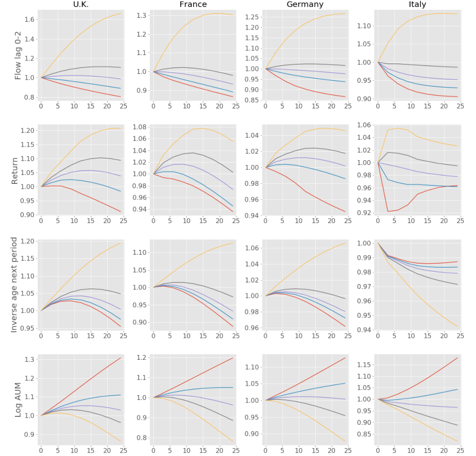
Note: The plots show forecast AUM time paths for each of the four fund domiciles. Each set of plots corresponds to a set of variables, whose average is divided into quintiles using data from the entire sample. The starting values for the variables are the mean within each quintile, while the starting values for the remaining variables are the means across the whole sample. The AUM is then forecast using the regression results in Table 3, assuming all future returns are equal to the sample mean, and all innovations in the autoregression specification are equal to zero. Each time path is rescaled, so that the initial AUM is equal to unity. The red, blue, lilac, grey and yellow lines correspond to the 1st, 2nd, 3rd, 4th and 5th quintiles respectively.
| Flow Flow | lag 1 Flow | lag 2 | Return Inv. | age Log | AUM | Flow Flow | lag 1 Flow | lag 2 | Return Inv. | age Log | AUM | |
|---|---|---|---|---|---|---|---|---|---|---|---|---|
| Q1 | -0.090 | -0.079 | -0.071 | -0.063 | 0.003 | 1.404 | -0.090 | -0.094 | -0.088 | -0.091 | 0.004 | 0.723 |
| Q2 | -0.031 | -0.024 | -0.021 | -0.009 | 0.005 | 1.988 | -0.028 | -0.028 | -0.026 | -0.010 | 0.006 | 1.318 |
| Q3 | 0.000 | 0.002 | 0.005 | 0.023 | 0.008 | 2.341 | -0.007 | -0.007 | -0.006 | 0.020 | 0.008 | 1.708 |
| Q4 | 0.033 | 0.033 | 0.037 | 0.052 | 0.012 | 2.651 | 0.015 | 0.017 | 0.017 | 0.049 | 0.012 | 2.077 |
| Q5 | 0.149 | 0.163 | 0.173 | 0.108 | 0.027 | 3.165 | 0.153 | 0.163 | 0.164 | 0.099 | 0.029 | 2.624 |
| Germany | Italy | |||||||||||
| Flow Flow | lag 1 Flow | lag 2 | Return Inv. | age Log | AUM | Flow Flow | lag 1 Flow | lag 2 | Return Inv. | age Log | AUM | |
| Q1 | -0.092 | -0.095 | -0.089 | -0.099 | 0.003 | 0.893 | -0.086 | -0.094 | -0.094 | -0.104 | 0.004 | 0.998 |
| Q2 | -0.034 | -0.032 | -0.033 | -0.011 | 0.005 | 1.392 | -0.035 | -0.045 | -0.053 | -0.021 | 0.005 | 1.553 |
| Q3 | -0.013 | -0.015 | -0.015 | 0.020 | 0.007 | 1.791 | -0.019 | -0.016 | -0.019 | 0.016 | 0.006 | 1.902 |
| Q4 | 0.006 | 0.007 | 0.006 | 0.048 | 0.011 | 2.223 | 0.009 | 0.014 | 0.012 | 0.044 | 0.009 | 2.267 |
| Q5 | 0.114 | 0.126 | 0.133 | 0.098 | 0.029 | 2.935 | 0.114 | 0.156 | 0.150 | 0.096 | 0.020 | 2.624 |
Note: The table shows the mean of each variable in each quintile as employed in the plots shown in Figure 2.
5. Conclusion
This note presents a forecasting analysis of AUM for funds domiciled in the UK, France, Germany and Italy. The forecasting approach consists of formulating equations for fund flow and fund returns. Fund flow is assumed to depend on a set of variables suggested by the substantial academic literature on these topics. Such variables include lagged fund flow, lagged returns, age, and size.
Non-linearity in the regression relationships (in particular for fund flows) are allowed for by using piecewise continuous transformations of the independent variables. The cut-off points for these transformations are motivated by non-parametric, univariate analysis of the fund flows and the regressor in question.
Since the primary purpose of our analysis is to supply methodologies that can be used in financial planning and stress testing for funds, we also include as regressors the macroeconomic variables: equity index returns and long and short interest rate changes. Typically, in stress tests, projections are performed conditional on these variables.
To understand the economic materiality of the regression results, we perform a set of impact response analyses. These consist of generating average forecast AUM time paths for funds (from each domicile) grouped into quintiles based on the regressor in question. This analysis is performed conditional on macroeconomic variables.
This analysis provides a series of conclusions about AUM dynamics. Qualitative patterns emerge for lagged fund flow, lagged return, age and size effects that are intuitive and similar for all domiciles. The only exception is age effects for Italian funds which suggest young funds grow less rapidly than old. This may reflect the difficult competitive position of young funds in the Italian market since the crisis.
The quantitative patterns implied by the impact response analysis suggest that, overall, lagged fund flow has the biggest effect although other variables imply significant impacts. UK funds are more sensitive to impact effects than funds from other domiciles.
This is most noticeable for lagged fund flow effects which imply future AUM growth ranging from plus 60% to minus 20% for average funds in the top and bottom lagged fund flow quintiles (over the full six year horizon of the simulation). For Italy, the least sensitive domicile, the range is from plus 13% to minus 9%. Again, for lagged return effects, the UK exhibits plus 20% and minus 10% for the highest and lowest lagged return quintiles compared to plus 3% to minus 4% for Italy.
6. References
Berk, Jonathan B., and Richard C. Green (2004) “Mutual fund flows and performance in rational markets,” Journal of Political Economy, Vol. 112, No. 6, pp. 1269-1295.
Bollen, Nicolas PB, and Jeffrey A. Busse (2004) “Short-term persistence in mutual fund performance,” Review of Financial Studies, Vol. 18, No.2, pp. 569-597.
Carhart, Mark M. (1997) “On persistence in mutual fund performance,” Journal of Finance, Vol 52, No. 1, pp. 57-82.
Chevalier, Judith, and Glenn Ellison (1997) “Risk taking by mutual funds as a response to incentives,” Journal of Political Economy, Vol. 105, No. 6, pp. 1167-1200.
Clifford, Christopher, et al. (2013) “Risk and fund flows,” Working paper.
Daniel, Kent, et al. (1997) “Measuring mutual fund performance with characteristic‐based benchmarks,” The Journal of Finance, Vol. 52, No. 3, pp. 1035-1058.
Del Guercio, Diane, and Paula A. Tkac (2008) “Star power: The effect of Morningstar ratings on mutual fund flow,” Journal of Financial and Quantitative Analysis Vol. 43, No. 4, pp. 907-936.
Fama, Eugene F., and James D. MacBeth (1973) “Risk, return, and equilibrium: Empirical tests,” Journal of Political Economy, Vol. 81, No. 3, pp. 607-636.
Goetzmann, William N., and Roger G. Ibbotson (1994) “Do winners repeat?” Journal of Portfolio Management, Vol. 20, No. 2, pp. 9-18.
Grinblatt, Mark, and Sheridan Titman (1992) “The persistence of mutual fund performance,” Journal of Finance, Vol. 47, No. 5, pp. 1977-1984.
Hendricks, Darryll, Jayendu Patel, and Richard Zeckhauser (1993) “Hot hands in mutual funds: Short‐run persistence of relative performance, 1974–1988,” Journal of Finance, Vol. 48, No. 1, pp. 93-130.
Huang, Jennifer, Kelsey D. Wei, and Hong Yan (2007) “Participation costs and the sensitivity of fund flows to past performance,” The Journal of Finance, Vol. 62, No. 3, pp. 1273-1311.
Jain, Prem C., and Joanna Shuang Wu (2000) “Truth in mutual fund advertising: Evidence on future performance and fund flows,” Journal of Finance, Vol. 55, No. 2, pp. 937-958.
Nanda, Vikram, Z. Jay Wang, and Lu Zheng (2004) “Family values and the star phenomenon: Strategies of mutual fund families,” Review of Financial Studies, Vol. 17, No. 3, pp. 667-698.
Petersen, Mitchell A. (2009) “Estimating standard errors in finance panel data sets: Comparing approaches,” Review of Financial Studies, Vol. 22, No. 1, pp. 435-480.
Sirri, Erik R., and Peter Tufano (1998) “Costly search and mutual fund flows,” Journal of Finance, Vol. 53, No. 5, pp. 1589-1622.
Risk Control Limited 13-14 Dean Street London W1D 3RS +44 (0)203 307 0730 www.riskcontrollimited.com
Notes
[1] This research note was prepared by Jozsef Kutas and William Perraudin. Note: This table shows regression results for each of the four fund domiciles included in the sample. The dependent variable is the contemporaneous quarterly fund flow. Lagged quarterly fund flows, lagged quarterly and annual returns, lagged log assets under management (EUR millions) and inverse age (months) are included as explanatory variables. Three macroeconomic variables are also included as explanatory variables: quarterly changes in the log of an equity index, in 3 month rates, and in 10 year rates.
[2] Any observations with missing data for one or more of the explanatory variables are dropped. The market data is not used in the simulation.