

Banks worldwide are implementing new approaches to measuring risk associated with the Environmental, Social and Governance features of their loan exposures. ESG adds an additional dimension of risk to the drivers that banks have traditionally considered: credit, market and operational.
Executive Summary
Banks worldwide are implementing new approaches to measuring risk associated with the Environmental, Social and Governance features of their loan exposures. ESG adds an additional dimension of risk to the drivers that banks have traditionally considered: credit, market and operational.
This paper develops a new approach to modelling ESG and credit risk within a common framework. The technique involves modelling ESG and credit ratings as correlated Markov chains, expanding the classic Ordered Probit approach to credit portfolio analysis by including an additional metric of issuer ESG status.
The models proposed are implemented statistically using historical data on Refinitiv (ESG) and Moody’s
(credit) ratings. The parameter estimations are performed using Maximum Likelihood techniques. The model allows for correlation between common factors driving credit and ESG ratings and for correlation between issuer-level idiosyncratic shocks.
Individual issuer ratings exhibit relatively low correlations (lower than those assumed in the Basel Internal Ratings Based Approach risk weights, for example). But a high and statistically significant correlation is evident between the common factors driving, respectively, credit and ESG ratings.
This suggests that, in a diversified bank portfolio, ESG and credit factors will jointly boost overall risk through their positively correlated common movements.
As a final exercise, we repeat the analysis but using E, S and G ratings (which we construct from the Refinitiv pillar scores) rather than the official Refinitiv ESG rating. This permits us to examine which aspects of the ESG ratings are correlated with credit ratings. In this, we find that the credit risk factor correlations are strongest with Environment and lowest with Governance.
This paper was prepared by:
• Dharshan Balasirishwaron, Imperial College, London;
• Georges Duponcheele, Risk Control; and
• William Perraudin, Risk Control.
Please address comments to:
georges.duponcheele@riskcontrollimited.com or william.perraudin@riskcontrollimited.com
1 Introduction
Banks worldwide are currently attempting to incorporate Environmental, Social and Governance (ESG) factors into the frameworks that they use to analyse loans. The traditional risk factors that banks reflect in pricing, provisioning, profitability and capital calculation are credit risk, market risk and operational risk. Including ESG as a risk factor expands the dimensionality of risk assessment, obliging banks, insurers and asset managers to reconsider how they should evaluate possible investments.
Modelling ESG risk remains at an early stage of development. To analyse ESG risk requires a clear understanding of how ESG factors affect the pricing of instruments. A companion paper to the present one analyses just that, in the context of corporate bonds. However, without making a full connection to pricing, one may still analyse ESG risk as it is reflected in ESG ratings. As an approach, this is particularly natural in banks for which credit ratings (internal or external) provide a central discipline for risk analysis and pricing.
This paper analyses the statistical properties of ESG ratings including their univariate behaviour (as reflected in transition matrices), and, more important for portfolio analysis, their correlations. Correlation, or more generally dependence, is a key aspect of risk since only risks that are correlated affect the riskiness of large, diversified portfolios of the sort that banks typically hold. In contrast, uncorrelated risks wash out as an institution diversifies its holdings.
Here, we analyse (i) how correlated are ESG risks across issuers and (ii) to what extent ESG risk is correlated with factors driving credit standing. We apply our approach to a large dataset of bond market issuers. The historical ESG ratings we employ are those provided by Refinitiv (formerly ASSET4). Berg et al. (2019) and Dimson, Marsh and Staunton (2020) comment on the significant disagreement on issuer ratings among ESG rating vendors. While important, this issue is of limited significance for us as we are, here, studying how one set of credit ratings is related to another set of ESG ratings. In the exercise we perform, we employ Moody’s ratings to measure credit standing. A bank starting its ESG integration work might prefer to determine any existing ESG relationship with its own ratings.
One may note that, unlike credit ratings which are not revisited, ESG ratings may be substantially re-written ex post if the rating agency involved changes its methodology or data sources. Depending on whether the original or rewritten data are used, rankings and classifications of firms into ESG quantiles may change. Berg et al.
(2021) demonstrate that these changes affect tests that relate ESG ratings to returns. Again, the observation is not so relevant for us as we are examining how (possibly re-written) ESG ratings historically were related to credit standing. It is, indeed, better for our exercise that the ESG ratings are derived from a single consistent methodology applied retrospectively.
Further note that there is an altogether different perspective that one may take to the link between ESG and credit ratings which is to seek to model jointly the determinants of each. For example, one may consider how heavy carbon consumption or more generally greater or lesser commitment to environmental aims affects credit risk. This amounts to examining credit risk conditional on observable ESG indicators. Such an approach has applications, for example in generalising a credit score card to allow for environmental risk affecting bond issuers. We intend in future to study these issues but here we restrict attention to the joint distribution of credit and ESG ratings rather than modelling one dimension of risk conditional on observable indicators related to the other.
Such conditional analysis is what Klein (2019) implements when he constructs a discriminant function that includes an ESG factor and found that it had a higher explanatory power in discriminating between industrial companies’ good and poor credit qualities than similar models that don’t include an ESG factor. Similarly, Devalle et al. (2017) investigates the linkage between ESG performance and credit ratings in Spain and Italy. They find no clear link between the cost of debt financing and ESG performance, but, for a subset of publicly rated companies, argue that ESG performance, as reflected, especially, in social and governance measures, meaningfully affects credit ratings. Aslan et al. (2021) perform a similar exercise with US firms and S&P credit ratings. They find the probability of corporate credit default to be significantly lower for firms with high ESG performance. Furthermore, by expanding the time window in their regression analysis, they observe that the influence of ESG and its constituents strongly varies over time. In a sector decomposition, they find that the energy sector is most influenced by ESG regarding the probability of corporate credit default.
This study is organised as follows. Section 2 explores the different data sets. Section 3 explains the methodology used. Section 4 provides the results.
2 ESG and Credit Ratings Data
2.1 ESG Rating Data
This section describes the data employed in the study. As already noted, this consists of historical Refinitiv ESG ratings and Moody’s credit ratings.
The ESG dataset covers 8,473 firms across 84 domiciles (countries), 5 regions and 11 economic sectors. The dataset offers several identifiers as well as ESG scores, such as industry group and ISINs, ranging from 2002 until 2019.
A Refinitiv ESG rating consists of a score between 0 and 100. The numerical scores are converted into one of 12 letter grades from D- to A+, hereafter referred to as ESG ratings, using a set of cut-off points. For example, a Drated company would have a score between 0 and 100/12, while a D rated company would have a score between 100/12 and 100/6, and so on. Refinitiv also provides individual E, S and G scores, constructed in a similar way, for each year. Here, we focus only on the overall ESG score.
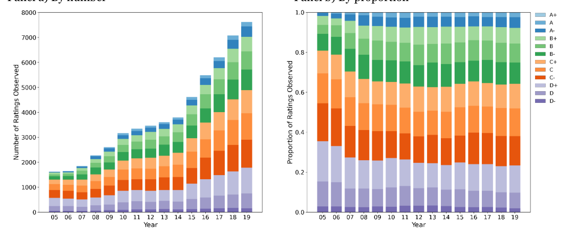
Figure 2.1 displays the distribution of ESG ratings by year, by number in Panel a) and by proportion in Panel b). For the purposes of evaluating more general transitions, we also consider the case of 4 ESG quartile letter ratings – A, B, C, D. To obtain these, we condensed the finer grades to a coarser set of categories. For example, D-, D and D+ ratings become D, etc. In this case, a D rated company would have a score falling between 0 and
25. In Figure 2.1, the split is represented by the colour (shades of blue, green, orange and purple, for the A, B, C and D category, respectively).
2.2 Credit Rating Data
We restrict our analysis to firms in the ESG rating dataset that have credit ratings from Moody’s. This subset is of size 1,050, representing just over 1/8 of the entire dataset. Also, data corresponding to the years 2002 – 2004 are excluded from the dataset, as we observe that a large number of credit ratings were withdrawn in 2005.
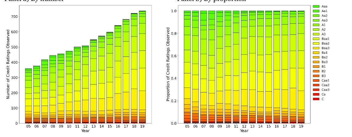
One may observe from Figure 2.2 a linear growth in the number of credit ratings. This, of course, reflects the fact that the number of ESG ratings grew through this period and, hence, entities with both ESG and credit ratings increased in number. The figure also reveals the low numbers of speculative grade issuers in our sample. This will have implications for the empirical analysis described below.
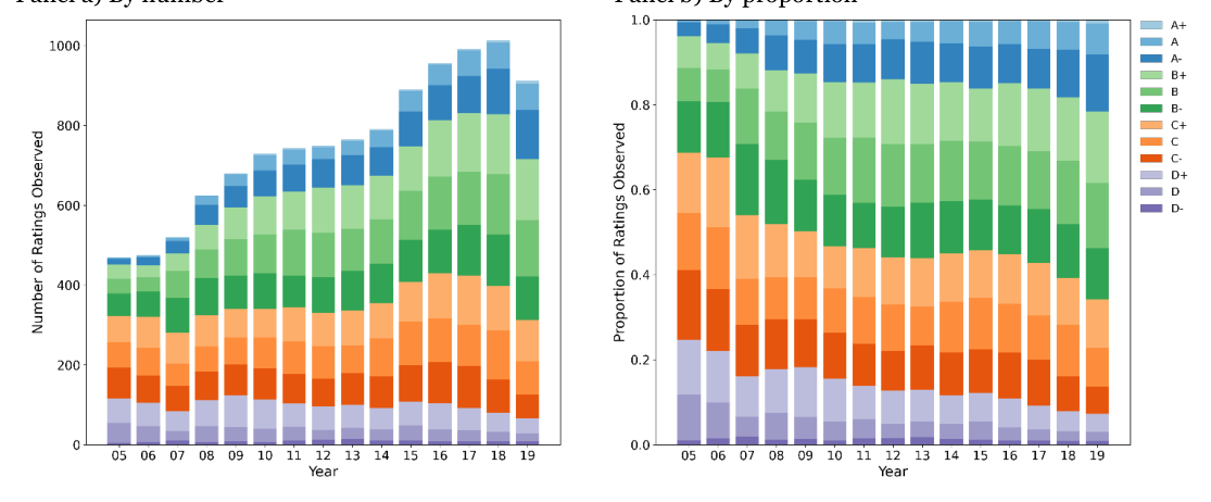
Conditioning our ESG dataset by excluding ESG-rated issuers that do not have credit ratings also changes the distribution of ESG ratings, as shown in Figure 2.3. There is now a clear trend in the ESG ratings for firms with credit ratings from Moody’s, in that the proportion of these firms that are ESG laggards decreases over time. In a similar way, the proportion of ESG leaders increases. Overall, these firms, as a group, have better ESG ratings when compared with the entire dataset and also exhibit improvement over time.[1]
than 10% of the dataset for any given year. The low percentage of speculative grade is reflective of ESG history. ESG concerns for many years were the preserve of large companies with strong cashflows. These tended to have investment grade ratings.
For completeness, we carry out our analysis twice, once on the entirety of the dataset, and once only using observations for which a firm begins a year with an investment-grade credit rating. This allows us to distinguish the specific behaviour of investment grade companies.
Note that the proportion of speculative grade companies – those with credit rating from Ba1 down to C – is less
2.3 ESG ratings conditional on Credit ratings
To explore the evolution of ESG rating trends, we subdivide the dataset into four credit rating groups:
1. ‘High Quality’ which refers to a credit rating from Aaa down to Aa3,
2. ‘Upper Medium Grade’ from A1 down to A3,
3. ‘Medium Grade’ from Baa1 down to Baa3, and
4. ‘Speculative Grade’ from Ba1 down to C.
Figure 2.4 shows the ESG quartile distributions for this grouping.
The top left panel for High Grade, shows a high proportion of the top ESG quartile letter rating ‘A’, suggesting that companies with higher credit quality are more likely to be ESG leaders than laggards.
The improvement trend in ESG ratings is more pronounced for the ‘Medium Grade’ corporates than the ‘Upper Medium Grade’ one, which is surprising, especially among the bottom ESG quartile letter rating ‘D’. It is almost as if a strong investment grade credit rating is less sensitive to ESG factors than a weak investment grade credit rating; in other words, companies that are at the frontier of investment grade and speculative grade make extra efforts to avoid being an ESG laggard in the event that this could tip the balance with the rating agencies and being pushed in the speculative grade category.
A small minority of the credit ratings are speculative-grade. This motivates our decision to run analysis excluding observations regarding speculative grade companies, as we observe a very small number of transitions from speculative grade credit ratings to investment grade.
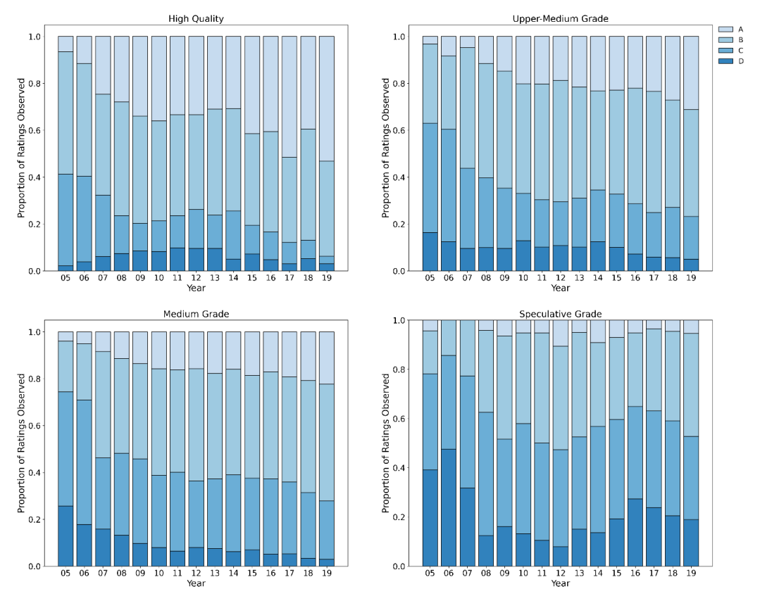
Note: ‘High Quality’ refers to a credit rating from Aaa down to Aa3, ‘Upper Medium Grade’ from A1 down to A3, ‘Medium Grade’ from Baa1 down to Baa, and ‘Speculative Grade’ from Ba1 down to C.
2.4 Exploratory analysis of ESG and Credit ratings
In this section, we examine properties of rating downgrade and upgrade rates for the ESG and credit ratings in order to understand their nature, as a preliminary to the formal statistical modelling presented in Sections 3 and 4 below. It is advisable to understand basic trends and tendencies in data of the type employed here in order to grasp how these properties are translated into estimated parameters in more complex models.
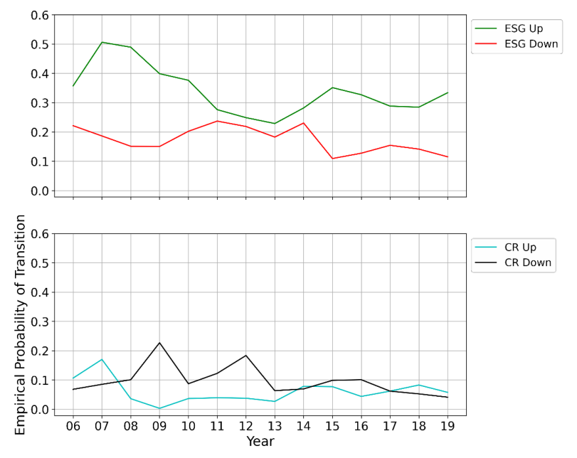
Figure 2.5 shows the evolution over time of empirical rating upgrade and downgrade probabilities. The ESG ratings in the sample generally upgrade more than downgrade, but when the proportion of upgrades declined, the proportion of downgrades increased, and likewise fell again once the proportion of upgrades increased after
2013. We see a similar pattern in credit ratings transitions, as they seem negatively correlated before remaining fairly constant after 2013. These patterns are consistent with there being common factors separately driving the credit and ESG ratings.
Table 2.1 presents the correlations for time series of upgrade and downgrade rates (i.e., empirical probabilities of upgrade and downgrade) for ESG and credit ratings. The most relevant results are the 36.95% and 13.05% correlations between upgrades and downgrades, respectively, in credit and ESG ratings. This suggests that the common factors driving ESG and credit ratings are positively correlated. Transition ESG Up ESG No Change ESG Down CR Up CR No Change CR Down ESG Up 1.0000 -0.8648 -0.2170 0.3695 -0.4223 0.1047 ESG No Change -0.8648 1.0000 -0.3025 -0.4102 0.5248 -0.1694 ESG Down -0.2170 -0.3025 1.0000 0.0961 -0.2186 0.1305 CR Up 0.3695 -0.4102 0.0961 1.0000 -0.3570 -0.4624 CR No Change -0.4223 0.5248 -0.2186 -0.3570 1.0000 -0.6632 CR Down 0.1047 -0.1694 0.1305 -0.4624 -0.6632 1.0000
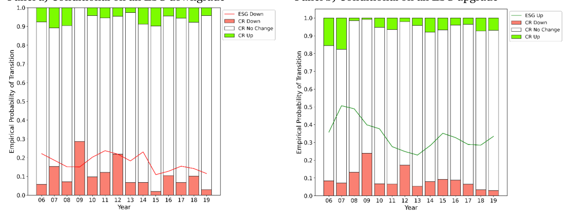
Finally, Figure 2.6 represents time series of credit rating transition probabilities, conditional on the firm in question having experienced an ESG downgrade (Panel a)) in the period in question and conditional on having experienced an ESG upgrade (Panel b)).
The results in Figure 2.6 are somewhat suggestive of a dependence between transitions in the two sets of ratings in that the red bars on the left appear to be on average greater in magnitude than the red bars on the right, while the opposite is true for the green bars. But the results are not very striking which suggests that the idiosyncratic risk in both sets of ratings is significant and so results do not show through strongly. More elaborate statistical modelling may be able to shed stronger light on the effects implicit within the data as we shall see in the next two sections.
3 Statistical Methods for ESG and Credit Rating Analysis
3.1 Summary of the modelling approach
The modelling approach presumes that ratings evolve as correlated Markov chains. Each issuer’s rating, both for ESG status and credit standing, stays constant or moves to a different value with probabilities specified in rating transition matrices which are constant over time.
For both ESG and credit ratings, we formulate the Markov chain using an Ordered Probit approach, also commonly referred to as the Creditmetrics model[2]. This permits one to allow for correlation between rating transitions of different issuers. We assume that for the two ratings, transitions are driven by Gaussian latent factors which include a common factor plus an idiosyncratic shock.
The standard Ordered Probit model applied to credit risk modelling allows for one or more common factors driving transitions in a portfolio of individual exposures with different ratings. Here, we assume that a single common factor drives credit rating transitions but that this factor can be correlated with another single factor that drives ESG rating transitions. We are particularly interested in the degree of correlation between the two common factors as this is potentially material for risk in a well-diversified bank portfolio with credit and ESG risk.
As a final generalisation of the modelling, we allow for non-zero correlation between the idiosyncratic shocks driving the credit and ESG ratings of individual bond issuers.
The estimation of the model is performed sequentially:
1. We estimate transition matrices for the two sets of ratings. We implement two approaches to estimating transition matrices. One approach is to take an average of the yearly respective transition matrices for ESG rating and credit rating, where we use empirical transition probabilities, and thus weighting each year equally. The second is to count all observations of rating transitions, and then use this information to create a matrix of empirical probabilities, thus weighting years by the number of observations.
2. We estimate the weights on the common factors driving the ESG and credit ratings, i.e., (i) the correlation between ESG rating transitions of individual issuers and (ii) correlation between credit rating transitions of individual issuers. In so doing, we assume that the transition matrix parameters are known.
3. We estimate the correlation between the two common factors that separately drive ESG and credit ratings.
4. We generalise the estimation approach implemented in the second and third steps described above by allowing for possible non-zero correlation between the idiosyncratic shocks for credit and ESG of individual borrowers.
Our implementation yields three models embodying the following assumptions:
• Model 1 – Independent idiosyncratic shocks and correlated common factors
• Model 2 – Independent common factors and correlated idiosyncratic shocks
• Model 3 – Correlated common factors and idiosyncratic shocks, i.e., the “full model”.
We fit each model for each of 8 cases. The eight cases correspond to three binary choices that we make:
1. Employ either 12 or 4 ESG quartile letter ratings,
2. Use different weightings for yearly observations,
3. Employ either all credit rating transitions or only transitions that start in investment grade.
3.2 Rating Dynamics
(*). Ratings take values in integer sets, Each firm n has a rating in period t for credit and ESG, R$,&((), R$,& {1,2, … , J(()}, {1,2, … , J(*)}, respectively. In each case, 1 indicates the highest rating. The J(() rating is absorbing.
(() drives the credit rating following one factor structure: We assume the latent variable X2$,&
(() (1) X2$,&(() = 4ρ(()f&(() + 41 −ρ(()ε$,&
((), firm n’s idiosyncratic shock for year t, are standard normal and Here f&((), a common factor for year t, and ε$,& (() is also standard normal. independent across t and n. ε$,&(() and ε:,&(() are independent. It follows that X2$,&
In a given year t, for firms m≠n, and m, n= 1, … , N:
(()B = ρ(() CorrAX2$,&((), X2:,& (()B = 0, s≠t CorrAX2$,&((), X2:,C (2) (()B = 0 CorrAε$,&((), ε:,& (()B = 0, s≠t CorrAε$,&((), ε:,C
(*) that drives ESG rating as: Similarly, we model X2$,&
(*) (3) X2$,&(*) = 4ρ(*)f&(*) + 41 −ρ(*)ε$,&
The evolution of rating changes follows a bivariate Markov Chain with transition matrices M(() and M(*).
(()] may be used to Credit ratings are modelled using an ordered probit approach. The elements of M(() = [ mI,J ((), i∈{1,2, … , J(() −1}, via: infer a set of cut-off points zI,J
J (() (() = ΦPQA∑ B (4) zI,J STQmI,S
Then the probability that a firm with rating i at time t has a rating j at time t+ 1 equals: (() B,for j∈(2, … , J−1} ΦAzI,J(()B −ΦAzI,JPQ (() Y , for j= J (5) 1 −ΦVzI,W(X)PQ (()B,for j= 1 ΦAzI,Q
We obtain similar expressions for ESG ratings also with similar ordered probit model with transition matrix (*)]. M(*) = [ mI,J(*)] used to infer cut-off points Z(*) = [ zI,J
3.3 Statistical Estimation
Denote by N(()(i, j, t), the number of observations for which a credit rating goes from i to j for a firm between the years t and t+ 1, and similarly N(*)(i, j, t) for ESG ratings.
Using the above assumptions, we arrive at the likelihood to observe historical data for credit rating transitions:
i(X)(I,Q,&) (X) (X)Pde(X)fg j W(X) ab,c k ∏ L(()(ρ(()) ≡∏&Tl ∫Pj ITQ Φ` h dQPe(X)
i(X)(I,J,&)
(X) (X) ⎪⎧ W(X)PQ ab,s(X)Pde(X)fg ab,stcPde(X)fg ⎪⎫ ∏ × JTv rΦ` h −Φ` hu dQPe(X) dQPe(X) ⎩⎪⎨ ⎭⎪⎬ i(X)(I,W,&) (X) (X) ab,z(X)tcPde(X)fg × r1 −Φ` hu φAf&(()Bdf&(() dQPe(X)
(6)
Here, we omit inconsequential scaling parameters. We have a similar expression for the likelihood of observing ESG ratings also. We estimate these parameters via maximum likelihood estimation, and, henceforth, will treat these parameters as known and constant for the purposes of further estimation.
For our first model, we assume that the factors f(() and f(*) have a correlation coefficient ρ. We now have the likelihood of observing the historical ratings experience of both credit and ESG rating, given ρ:
i(})(I,Q,&) (}) (}) ⎪⎧ ⎪⎧ ⎪⎧ j j W(}) ab,c(})Pde(})fg W(})PQ ab,s(})Pde(})fg k ∏ ∏ ∏ L(ρ) ≡∏&Tl∫Pj ∫Pj ~T*,( ITQ Φ` h × JTv rΦ` h − dQPe(}) dQPe(}) ⎩⎪⎨ ⎩⎪⎨ ⎩⎪⎨ i(})(I,J,&) i(})AI,W(}),&B (}) (}) (}) ⎪⎫ a Pde(})fg ⎪⎫⎪⎫ ab,stcPde(})fg b,z(})tc Φ` hu × r1 −Φ` hu φAf&((), f&(*)•ρBdf&(()df&(*) (7) dQPe(}) dQPe(}) ⎭⎪⎬ ⎭⎪⎬⎭⎪⎬
For our second model, we now instead assume that the common factors are independent, and it is instead the (*), and with slight idiosyncratic shocks that are correlated with parameter ρI. Note that yI,J(*) is dependent on f& abuse of notation we define them: (() = −∞, yI,l
(X) ab,s(X)Pde(X)fg (() = , for j= 1, ⋯, J(() −1 (8) yI,J dQPe(X)
(() = ∞ yI,W(X)
(*). Denote by N(i, j, k, l, t) the number of observations for which a firm’s ESG rating And we similarly define yS,ƒ transitions from state i to j and credit rating transitions from state k to l between the years t and t+ 1. Let Φv( ⋅ , ⋅│ρIˆ) be the Cumulative Distribution Function (CDF) for a standard bivariate Gaussian with correlation ρIˆ. We now arrive at a new likelihood:
j j W(Œ) W(X)PQ W(Œ) W(X) k LAρIB ≡ ∏&Tl ∫Pj ∫Pj ‰∏ITQ ∏STQ ∏JTQ ∏ƒTQ ŠΦv VyI,J(*), yS,ƒ(()‹ρIˆY −Φv VyI,JPQ(*) , yS,ƒ(()‹ρIˆY − i(I,J,S,ƒ,&) (*) (9) (() ‹ρIˆY• Φv VyI,J(*), yS,ƒPQ(() ‹ρIˆY + Φv VyI,JPQ(*) , yS,ƒPQ ŽφVf&(*)Y φVf&(()Y df&(()df&
Our final model modifies this model to maintain the assumption of imperfect correlation of common factors by (*)•ρB. replacing φAf&(*)BφAf&(()B with φAf&((), f&
3.4 Numerical Implementation
We create an array to count the joint transitions between ESG and Credit ratings, i.e., an array composed of elements N(i, j, k, l, t) as described previously. From here we have two approaches to generate overall transition matrices for ESG ratings and credit ratings. For credit ratings, we sum over i and j to produce T count matrices for credit transitions, where T is the number years, i.e., a count matrix for each year, each k × l.
Weighting each year equally, we may convert each count matrix to a transition matrix by dividing each row by their respective row sums, and then averaging these matrices. If we instead choose not to weight each year equally, we sum our T count matrices and then convert to a transition matrix by dividing each row by their respective row sums. We repeat the same procedure for ESG ratings, but sum over k and l to begin with instead of i and j.
We then extracted inferred cut-off points from the transition matrices, for use in the likelihood functions. For the purposes of avoiding zero errors and underflow issues, any 0 probabilities in our transition matrices are replaced with a very small number, and each row is rescaled to sum to 1 again – this in practice will not change results very much. In all likelihood functions, the outer integrals are computed using Gaussian-Hermite quadrature, and we employ an interpolation-based approach to evaluate the Gaussian bivariate CDFs in the idiosyncratic shock correlation likelihood function.
We do this by evaluating 25,000 points from the standard bivariate Gaussian with correlation ρIˆ, and using this grid of sample points to estimate the CDFs, to improve the speed of computation. We take the negative logarithm of all these likelihood functions and feed them into a minimiser to find the MLE. We estimate standard error by taking the square root of the inverse Hessian returned by the minimiser.
4 Results
This section presents the results of the statistical analysis. As explained above, we estimate three models under eight different sets of assumptions (so, 24 models in all). The eight sets of assumptions correspond to the possible values of three binary choices:
1. Whether to use Refinitiv’s suggested 12 ESG quantiles or use 4 ESG categories,
2. Whether each year should be weighted equally in our transition matrix calculation and
3. Whether all ratings data should be employed or just observations that start in an investment grade rating category.
Recall that the three models correspond to the cases in which
(a) Common factors are correlated across credit and ESG ratings but idiosyncratic shocks are uncorrelated,
(b) Common factors are uncorrelated across rating types but idiosyncratic shocks are correlated with any given time period for any given issuer, and
(c) The full model in which both types of correlation are included.
Our findings when all ratings data are employed (see binary choice 3) are presented in Table 5.1. The Table displays results based on use of 12 and 4 ESG categories and with two different weighting approaches for the transition matrix estimation, i.e., four sets of results in all. Table 5.2 shows results comparable to those presented in Table 5.1 but for observations corresponding to investment grade firms only (the other possibility in binary choice 3). The results are quite comparable to those shown in Table 5.1, confirming the stability of the findings in this respect, although as we comment below, the results based on Investment Grade borrowers appear less noisy so correlations are stronger and statistical significance levels higher.
Points implied by the results in Tables 5.1 and 5.2 include:
• In Table 5.1, the estimated factor weights (i.e., the correlations for pairs of credit ratings or pairs of ESG ratings) appear relatively low, for example, 6.23% and 2.46% are the credit and ESG factor weights, respectively (with equally weighted transition matrices and 4 ESG rating categories). The equivalent figures for investment grade firms only (in Table 5.2) are 6.76% and 2.05%. The credit risk factor weights may be compared to the factor correlations employed within the Basel Internal Ratings Based Approach corporate risk weight formula which range from 12% to 24% depending on the default probability of the firm in question.[3]
• While the latent variables driving ratings for individual exposures have low weights (as just noted), the correlation between the ESG and the credit common factors are high, being, for all credit grades (see Table 5.1), 41.74% for Model 1 in the case of equally weighted transition matrices and 4 ESG rating categories, and 37.10% in Model 3 (the “full model”). For investment grade firms alone (see Table 5.2), the equivalent figures are 55.62% and 55.49%.
• The idiosyncratic shock correlation is small, being, for all credit grades (Table 5.1) 2.43% in Model 2 and 2.42% in Model 3 when equally weighted transition matrices and 4 ESG rating categories are employed. The equivalent for investment grade firms (see Table 5.2) are 2.71% and 2.67%.
• Comparing the results with all credit grade firms (Figure 5.1) to those for Investment Grade firms alone (Figure 5.2), one may observe that the factor correlations are higher and significance levels greater. So, for example, for 4 ESG quantiles with equally weighted years, the Credit-ESG factor correlation is 55.62% in Table 5.2 with a t-statistic of 2.26 compared to 41.74% in Table 5.1 with a t-statistic of 1.40. This finding is intuitive since the presence of sub investment grade borrowers probably injects noise into the estimation, reducing the precision of estimates.
Note that the relative magnitudes of factor weight and correlations estimates are similar whether transition matrices are based on equal yearly weights or weights derived from numbers of observations. But in the former case, the magnitudes of the estimates are mostly higher. However, standard errors for some “full model” parameters are rather high leading to low t statistics. This problem is alleviated when 4 ESG categories are employed.
Table 5.3 presents results for Models 1 and 2 based on separate ratings for the three categories of Environmental, Social and Governance (rather than a single ESG rating). The individual pillar ratings are constructed using the same approach that is taken by Refinitiv for the full ESG rating (i.e., based an equal division of the zero to unity interval) but is applied to the three pillar scores reported by Refinitiv.
Estimates are presented in Table 5.3 for 12 and for 4 ESG rating categories. In all cases, the transition matrix estimates are weighted by number of observations. There are, hence, results for six models displayed in the table.
Key aspects of the results in Table 5.3 may be summarised as follows.
• The factor weights for Credit, Environmental and Social factor weights are all significantly different from zero according to the t-statistics. The Governance factor weights are not statistically significant in the case with 12 quantiles. In the case with 4 quantiles, the estimated Maximum
Likelihood factor weight estimate equals zero. A zero factor weight value implies that the creditgovernance correlation parameter is unidentified statistically. Its value (which is 72.97%), therefore, has no meaning and should be disregarded.
• Governance issues may be an important risk factor for many firms (and as such is often included in credit rating assessments) but our results suggest that this risk is less correlated across firms than environmental and social risks.
• The idiosyncratic shock correlation parameters for the three pillar ratings are 3.66%, 1.59% and 3.23% for Environmental, Social and Governance, respectively, and is statistically significant for Governance when 12 quantiles are employed.
| Parameter | Estimate StD | Error | t-Statistic | ||||
|---|---|---|---|---|---|---|---|
| Credit Rating | Factor | Weight | 0.0543 | 0.0154 | 3.5226 | ||
| ESG Rating | Factor | Weight | 0.0214 | 0.0086 | 2.4968 | ||
| quantiles, years weighted by | Model 1: | Credit-ESG | Factor | Correlation | 0.2800 | 0.2689 | 1.0413 |
| observations | Model 2: | Idiosyncratic | Shock | Correlation | 0.0223 | 0.0200 | 1.1120 |
| Model 3: Full | Model | Factor | Correlation | 0.2826 | 0.7661 | 0.3689 | |
| Model 3: Full | Model | Shock | Correlation | 0.0222 | 0.0221 | 1.0021 | |
| Credit Rating | Factor | Weight | 0.0623 | 0.0171 | 3.6411 | ||
| ESG Rating | Factor | Weight | 0.0606 | 0.0233 | 2.6071 | ||
| Model 1: | Credit-ESG | Factor | Correlation | 0.3793 | 0.3265 | 1.1617 | |
| years weighted equally | |||||||
| Model 2: | Idiosyncratic | Shock | Correlation | 0.0251 | 0.0203 | 1.2358 | |
| Model 3: Full | Model | Factor | Correlation | 0.3893 | 0.3181 | 1.2238 | |
| Model 3: Full | Model | Shock | Correlation | 0.0252 | 0.0201 | 1.2578 | |
| Credit Rating | Factor | Weight | 0.0543 | 0.0154 | 3.5226 | ||
| ESG Rating | Factor | Weight | 0.0159 | 0.0078 | 2.0321 | ||
| quantiles, years weighted by | Model 1: | Credit-ESG | Factor | Correlation | 0.3807 | 0.2791 | 1.3638 |
| observations | Model 2: | Idiosyncratic | Shock | Correlation | 0.0207 | 0.0252 | 0.8212 |
| Model 3: Full | Model | Factor | Correlation | 0.3524 | 0.3160 | 1.1153 | |
| Model 3: Full | Model | Shock | Correlation | 0.0204 | 0.0375 | 0.5440 | |
| Credit Rating | Factor | Weight | 0.0623 | 0.0171 | 3.6411 | ||
| ESG Rating | Factor | Weight | 0.0246 | 0.0157 | 1.5646 | ||
| Model 1: | Credit-ESG | Factor | Correlation | 0.4174 | 0.2981 | 1.4001 | |
| years weighted equally | |||||||
| Model 2: | Idiosyncratic | Shock | Correlation | 0.0243 | 0.0256 | 0.9488 | |
| Model 3: Full | Model | Factor | Correlation | 0.3710 | 0.3392 | 1.0940 | |
| Model 3: Full | Model | Shock | Correlation | 0.0242 | 0.0255 | 0.9471 | |
| Rating Factor Weight | correspond to | ρ(()/ρ(*) | respectively, as described | in the methodology. | These | weights |
Note: Credit/ESG Rating Factor Weight correspond to ρ(()/ρ(*) respectively, as described in the methodology. These weights are held as constant for each of the three models, and are estimated before any further parameters are. Similarly, Credit-ESG Factor Correlation and Idiosyncratic Shock Correlation correspond to ρ and ρIˆ. Weighting of years refers to how overall transition matrices are calculated for rating transitions, where equally weighted is an average of yearly transition matrices, while weighted by observation uses a transition matrix generated by all observed transitions across all years, thus weighting each year by the number of observations within a year.
| Maximum Likelihood | Estimates for | investment | grade firms | ||||
|---|---|---|---|---|---|---|---|
| Parameter | Estimate StD | Error | t-Statistic | ||||
| Credit Rating | Factor | Weight | 0.0567 | 0.0162 | 3.5029 | ||
| ESG Rating | Factor | Weight | 0.0198 | 0.0083 | 2.3829 | ||
| quantiles, years weighted by | Model 1: | Credit-ESG | Factor | Correlation | 0.3374 | 0.2628 | 1.2841 |
| observations | Model 2: | Idiosyncratic | Shock | Correlation | 0.0231 | 0.0203 | 1.1367 |
| Model 3: Full | Model | Factor | Correlation | 0.3200 | 0.3424 | 0.9347 | |
| Model 3: Full | Model | Shock | Correlation | 0.0230 | 0.0216 | 1.0612 | |
| Credit Rating | Factor | Weight | 0.0676 | 0.0183 | 3.6853 | ||
| ESG Rating | Factor | Weight | 0.0518 | 0.0246 | 2.1091 | ||
| Model 1: | Credit-ESG | Factor | Correlation | 0.4455 | 0.2881 | 1.5462 | |
| years weighted equally | |||||||
| Model 2: | Idiosyncratic | Shock | Correlation | 0.0242 | 0.0212 | 1.1373 | |
| Model 3: Full | Model | Factor | Correlation | 0.3928 | 0.4004 | 0.9809 | |
| Model 3: Full | Model | Shock | Correlation | 0.0242 | 0.0297 | 0.8169 | |
| Credit Rating | Factor | Weight | 0.0567 | 0.0162 | 3.5029 | ||
| ESG Rating | Factor | Weight | 0.0150 | 0.0077 | 1.9563 | ||
| quantiles, years weighted by | Model 1: | Credit-ESG | Factor | Correlation | 0.5173 | 0.2490 | 2.0779 |
| observations | Model 2: | Idiosyncratic | Shock | Correlation | 0.0253 | 0.0263 | 0.9606 |
| Model 3: Full | Model | Factor | Correlation | 0.5141 | 0.2472 | 2.0799 | |
| Model 3: Full | Model | Shock | Correlation | 0.0248 | 0.0259 | 0.9583 | |
| Credit Rating | Factor | Weight | 0.0676 | 0.0183 | 3.6853 | ||
| ESG Rating | Factor | Weight | 0.0205 | 0.0125 | 1.6346 | ||
| Model 1: | Credit-ESG | Factor | Correlation | 0.5562 | 0.2458 | 2.2628 | |
| years weighted equally | |||||||
| Model 2: | Idiosyncratic | Shock | Correlation | 0.0271 | 0.0268 | 1.0134 | |
| Model 3: Full | Model | Factor | Correlation | 0.5549 | 0.2385 | 2.3267 | |
| Model 3: Full | Model | Shock | Correlation | 0.0267 | 0.0256 | 1.0435 |
| Assumption | Parameter | Estimate StD | Error | t-Statistic | |||
|---|---|---|---|---|---|---|---|
| Credit Rating Factor | Weight | 0.0562 | 0.0166 | 3.3751 | |||
| 12 Environmental | quantiles, years | Environmental Rating | Factor | Weight | 0.0295 | 0.0110 | 2.6901 |
| weighted | by observations | Model 1: Credit-E | Factor | Correlation | 0.3271 | 0.2573 | 1.2714 |
| Model 2: Idiosyncratic | Shock | Correlation | 0.0287 | 0.0218 | 1.3191 | ||
| Credit Rating Factor | Weight | 0.0567 | 0.0162 | 3.5029 | |||
| 12 Social | quantiles, years weighted by | Social Rating Factor | Weight | 0.0230 | 0.0091 | 2.5290 | |
| observations | Model 1: Credit-S | Factor | Correlation | 0.2648 | 0.2725 | 0.9718 | |
| Model 2: Idiosyncratic | Shock | Correlation | 0.0228 | 0.0208 | 1.0944 | ||
| Credit Rating Factor | Weight | 0.0567 | 0.0162 | 3.5029 | |||
| Governance | quantiles, years weighted | Governance Rating | Factor | Weight | 0.0021 | 0.0020 | 1.0870 |
| by | observations | Model 1: Credit-G | Factor | Correlation | 0.2759 | 0.4442 | 0.6210 |
| Model 2: Idiosyncratic | Shock | Correlation | 0.0362 | 0.0198 | 1.8240 | ||
| Credit Rating Factor | Weight | 0.0562 | 0.0167 | 3.3691 | |||
| 4 Environmental | quantiles, years | Environmental Rating | Factor | Weight | 0.0297 | 0.0126 | 2.3673 |
| weighted | by observations | Model 1: Credit-E | Factor | Correlation | 0.2733 | 0.2770 | 0.9866 |
| Model 2: Idiosyncratic | Shock | Correlation | 0.0366 | 0.0267 | 1.3685 | ||
| Credit Rating Factor | Weight | 0.0567 | 0.0162 | 3.5029 | |||
| 4 Social quantiles, | years weighted by | Social Rating Factor | Weight | 0.0234 | 0.0101 | 2.3137 | |
| observations | Model 1: Credit-S | Factor | Correlation | 0.4423 | 0.2497 | 1.7709 | |
| Model 2: Idiosyncratic | Shock | Correlation | 0.0159 | 0.0259 | 0.6128 | ||
| Credit Rating Factor | Weight | 0.0567 | 0.0162 | 3.5029 | |||
| Governance | quantiles, years weighted | Governance Rating | Factor | Weight | 0.0000 | 1.0000 | 0.0000 |
| by | observations | Model 1: Credit-G | Factor | Correlation | 0.7297 | 0.6465 | 1.1287 |
| Model 2: Idiosyncratic | Shock | Correlation | 0.0323 | 0.0230 | 1.4028 |
Note: These estimates are calculated by converting E, S and G pillar scores respectively into ratings as we previously did for ESG scores. The analysis is then identical, simply substituting ESG ratings with pillar ratings.
5 Conclusion
Credit rating agencies and ESG rating agencies insist on the methodological differences between both assessments. Credit ratings and ESG ratings serve different purposes. Credit ratings are about the financial strength of a corporate and its ability to repay debt. ESG ratings, however, are a sort of metrics about the longterm business environment of a particular corporate. This in turn can indirectly affect, to a limited extent, the long-term financial prospects which are not currently expressed in standard credit models.
This paper seeks to contributes to an emerging literature on how risk associated with ESG status should be incorporated into broader risk management frameworks operated by financial institutions. Our immediate focus is on risk assessment by banks of their loan portfolios but the analysis we present has implications also for other financial institutions such as investment funds and insurers.
Different approaches may be taken to integrating ESG risk with other types of risk within a risk framework:
1. Some view ESG risk as a sub-category of credit risk (or more generally of payoff-performance risk for financial assets including equities) contributing to risk to the extent that it influences default likelihood or the Loss Given Default rate. In this case, one might argue that the correct adjustment for a bank’s risk management framework is to include ESG indicators within existing credit scorecards.[4] One may note that governance indicators are already included in many bank credit rating scorecards while environmental or ‘transition’ risk may or may not be included. (If, as is common, a one-year horizon is employed for risk management, the bank may consider that transition risk contributes little to pure default risk.) Social risk rarely figures in bank credit scorecards.
2. On the other hand, some believe that ESG affects the market pricing of debt instruments even allowing for such indicators of payoff risk as credit ratings (which may be taken to describe the payoff distribution of the exposures).[5] This may be because ESG affects risk premia (or Unexpected Losses) on debt instruments or because investors view high ESG scores as a ‘merit good’ in their portfolios and, hence, bid up the prices even though they do not view the value of ESG as reflected in Expected or Unexpected Losses. Such ideas are explored by studies including Pederson, Fitzgibbons and Pomorski (2020) and Ahmed, Gao and Satchell (2021)
The approach taken in this paper, represents a coherent response to ESG risk management for any case in which ESG factors affect market pricing over and above traditional credit ratings. In such a case, one can analyse the combined credit and ESG risk by modelling the joint behaviour of credit and ESG ratings.
Just as in the standard Ordered Probit (or Creditmetrics) model, one may simulate these two dimensions of risk and then calculate the impact on the value of the portfolio in question, applying spreads conditional on credit and ESG ratings. In a companion paper, to be issued shortly, we show that ESG is, indeed, reflected in the market pricing of publicly traded bonds, allowing for credit status as registered by credit ratings and, hence, we provide the other element necessary to the full implementation of this risk management approach.
Thus, our paper represents a step in the construction of appropriate risk tools for a world in which banks and others wish to allow for ESG risk. It also provides insight into the nature of ESG risk, demonstrating that ESG aspects are described by common risk factors related to, but distinct from, credit risk as reflected in traditional agency ratings.
References
Ahmed, M. F., Y. Gao and S. Satchell (2021) “Modelling Demand for ESG,” European Journal of Finance.
Aslan, A., L. Poppe and P. Posch (2021) “Are Sustainable Companies More Likely to Default? Evidence from the Dynamics between Credit and ESG ratings,” Sustainability, 13, 8568, July.
Barth, F., B. Hubel and H. Scholz (2021) “ESG and Corporate Credit Spreads,” mimeo.
Berg, F., K. Julian and R. Roberto (2019) “Aggregate Confusion: The Divergence of ESG Ratings,” MIT Sloan School Working Paper 5822-19, August
Berg, F., K. Fabisik and Z. Sautner (2020) “Re-writing History II: The (Un)Predictable Past of ESG Ratings,” European Corporate Governance Institute – Finance, Working Paper 708/202, November
Devalle, A., S. Fiandrino and V. Cantino (2017) “The Linkage between ESG Performance and Credit Ratings: A Firm-Level Perspective Analysis,” International Journal of Business and Management; Vol.12, No. 9; 2017, August.
Dimson, E., P. Marsh and M. Staunton (2020) “Divergent ESG ratings,” The Journal of Portfolio Management, 47 (1), 75-87.
Duponcheele, G. and W. Perraudin (2021), “ESG Strategy for Banks: Tackling the Data Problem”, Public Note 21-80a, Risk Control Limited, www.riskcontrollimited.com
Gordy, M., and E. Heitfield (2002) “Estimating default correlations from short panels of credit rating performance data,” Working paper, Federal Reserve.
Gupton, G. M., C. C. Finger, and M. Bhatia (1997) “Creditmetrics: Technical Document,” Discussion paper, J.P. Morgan, New York, April.
Jang, G., H. Kang, J. Lee and K. Bae (2020) “ESG Scores and the Credit Market,” Hanyang University Business School Department of Finance, April.
Klein, C. (2019) “Quantitative Credit Rating Models including ESG factors,” University of Stuttgart Faculty of Business and Social Science, Research Report No. 01/2019, September.
Mendiratta, R., H.D. Varsani and G. Giese (2020) “Foundations of ESG investing in Corporate Bonds: How ESG affected Corporate Credit Risk and Performance,” November.
Michalski, L., and L. Y. K. Rand (2021) “Corporate Credit Rating Feature Importance: Does ESG Matter?”, August.
Okimoto T. and S. Takaoka, T. (2021) “Sustainability and Credit Spreads in Japan,” RIETI Discussion Paper Series 21-E-052, July.
Pederson, L., S. Fitzgibbons and L. Pomorski (2020) “Responsible Investing: the ESG-Efficient Frontier,” Journal of Financial Economics, November, 142(2) 572-597.
Refinitiv (2021) “Environmental, Social and Governance (ESG) Scores from Refinitiv,” February, available at: https://www.refinitiv.com/content/dam/marketing/en_us/documents/methodology/refinitiv-esg-scoresmethodology.pdf
Yang, R. and Z. Li (2020) “Credit Ratings in the Age of Environmental, Social, and Governance (ESG),” April.
Appendix 1: Ratings by Sector and Region
A1. ESG ratings conditional on Economic sectors We further investigate the distribution of ESG ratings for investment grade firms in regards to economic sectors. By conditioning our ESG dataset to those firms with credit ratings from Moody’s, we lose one of the 11 economic sectors originally represented, namely Academic & Educational Services, of which there were only 30 of the original 8,473 companies. Figure A1.1 shows the ESG rating distributions for the remaining 10 sectors.
Figure A1.1: Economic sectoral breakdown of ESG quartile letter rating distribution
Of the sectors for which data appears in Figure A1.1, Real Estate companies have a larger share of ESG laggards than most. Additionally, the Healthcare sector sees stark improvements over the years, to the point of no ESG laggards in 2014, and from 2016 onwards. In contrast, the Energy sector sees improvements at the top end with a greater proportion of ESG leaders, but a fairly consistent proportion of laggards from 2007 onwards. There are also general improvements for sectors such as Financials, Consumer Cyclicals and Consumer Non-Cyclicals, though gradual. Analysis at a sectoral level may be relevant for firms wishing to better understand both ESG and credit rating dynamics specific to their own sector.
A1.2 ESG ratings conditional on Regions Figure A1.2 shows the distribution of ESG ratings for each continental region, Africa, Asia, Europe, Americas, Oceania. The data for Africa and Oceania is small, and thus the results will be mostly based upon the behaviour for firms in Asia, Europe and the Americas.
Figure A1.2: Regional ESG quartile letter rating distributions
Risk Control 13-14 Dean Street London W1D 3RS +44(0)2033070730 www.riskcontrollimited.com
Notes
[1] The total numbers of yearly observations in the left hand panels in Figures 2.2 and 2.3 do not match because Figure 2.2 counts the number of credit ratings available each year conditional on having had an ESG rating at some point in the sample period, while Figure 2.3 counts the number of ESG ratings for all firms that have had a credit rating at some point in the sample period. Note: Pearson product-moment correlation coefficients for the yearly proportions of rating transitions that were upgrades, downgrades or didn’t change for ESG and credit ratings. ESG Up/Down refer to ESG upgrades/downgrades and similarly for credit rating.
[2] See Gupton, Finger, and Bhatia (1997).
[3] It is well known among industry analysts that the correlations obtained from historical data are commonly much less than the correlations assumed in the Basel formulae. When regulators calibrated the Basel II Internal Ratings Based Approach Risk Weight formula (which is an analytical expression for Marginal Value at Risk capital assuming default risk alone), the correlations were set so that the implied capital charges were comparable to those implied by a ratings-based Ordered Probit model, i.e., inclusive of transition risk. Hence, the correlations were not directly based on the correlation data implicit in historical data but were more conservative.
[4] Yang and Li (2021) discuss the inclusion of ESG factors in the scorecards of the major rating agencies and whether this contributes to better predictive performance of credit events. Michalski and Rand (2021) seek to predict agency ratings using variables including ESG indicators.
[5] See, for example, Okimoto and Takaoka (2021) who analyse Japanese corporate bond spreads conditional on ratings and find spreads are negatively related to poor ESG performance. On the other hand, Seltzer, Starks and Zhu (2021) provide evidence that exposure to climate risk results in lower ratings and higher spreads, without trying to determine whether climate risk affects spreads over and above what one may expect from the credit rating. Barth, Hubel and Scholz (2021) show that Credit Default Swap (CDS) spreads are related to ESG indicators. In their regressions, they condition on variables (such as financial ratios) that may reflect credit risk but not on ratings. A different perspective on ESG ratings and debt markets is provided by Jang et al (2020) who examine the effect of ratings and ESG indicators on bond returns. Mendiratta, Varsani and Giese (2020) discuss how ESG factors may affect aspects of debt instruments important to investors including Expected Payoffs, idiosyncratic and factor risk. They argue that ESG ratings and complementary to credit ratings in providing information on these attributes. Jang, et al. (2020) argue that ESG indicators provide information about downside risk in Korean corporate bond returns and, as such, complement credit ratings.