

This note presents an illustrative case study of stress testing for an asset manager accomplished using Risk Control‟s Stress ControllerTM software. The calculations are performed for a notional UK asset manager that is also engaged in private banking operations.
1. Executive Summary
This note presents an illustrative case study of stress testing for an asset manager accomplished using Risk Control‟s Stress ControllerTM software. The calculations are performed for a notional UK asset manager that is also engaged in private banking operations.
We show how the AUM (Assets under Management), balance sheet, P&L and key capital planning ratios of the private bank-asset manager group are affected by scenarios involving (i) customer loss and (ii) a UK recession. A set of equations is constructed to describe the evolution of the asset manager‟s financial statements.
The AUM is modelled in a region- and asset-class-specific fashion. This permits the user to calibrate the distributions of the AUM across regions and to employ appropriate sensitivities of the AUM in each region to appropriate geographically specific market variables (equity indices, interest rates, exchange rates and commodity prices).
The growth of each AUM class is forecast by taking into account (i) changes in relevant market prices and (ii) user-specified additional growth reflecting, for example, past trends in AUL market growth or anticipated marketing activities by the asset manager. The model allows the user to override forecasts by directly assuming particular levels of AUL growth for different components of the AUL asset class-region breakdown.
Revenue in the form of fees depends on the AUM forecasts described above. Users are able also to specify fee rate dynamics directly if they wish, calibrating either the relative growth or the absolute level of the future fee rate.
The results show how the asset manager‟s AUM size, revenue growth, loan impairment provisions and capital are boosted or depressed by the different stress scenarios.
Note that the framework described here may be used either with coarse, public data to perform high level, top down stress testing or with highly granular internal data for bottom-up stress testing purposes. Financial statement modelling is highly flexible since equations may be written first in Excel, before being converted into scripts and then imported into the software for use at run-time to perform calculations.
2. Generating Consistent Macroeconomic Scenarios
The stress tests considered in this note include what one might term “parametric stresses” such as assumed changes in fee rates, for example, and also more economically based stress scenarios in which the consequences for the business of changes in the macroeconomic environment are traced through.
To devise economic stress tests of this latter type, one must first accomplish the (often challenging) task of generating consistent time paths for multiple macroeconomic variables. For example, one may wish to consider the impact of a recession in the US affecting, say, US GDP. However, this raises the issue of what the impact on European or Asian GDP should be and also what should happen to commodity prices and interest rates, exchange rates, inflation and in the different regions?
Risk Control‟s Stress ControllerTM software employs an embedded macroeconomic model which permits the user to specify shocks to a particular variable and then calculate conditional forecasts of this and other variables stretching into the future. The macroeconomic model employed is a statistical model commonly referred to as a Global Vector Autoregressive or GVAR model. Such models have been extensively used by central banks, government agencies and private sector analysts in economic forecasting and stress testing applications.
It is important to allow for contagion between regions in the propagation of macroeconomic scenarios. GVAR models suppose that for each geographical region there exists a vector of macroeconomic variables which evolve linearly over time as non-stationary but co-integrated time series. The variables in each region are affected by their own lagged values as well as by weighted sums of variables from other regions.
The GVAR model included in Stress ControllerTM is highly flexible in that one may readily change the countries and regions used. In the exercise reported in this note, we adopt a set of regions consistent with the bank‟s approach to categorizing its loan exposures. Specifically, we suppose that the regions comprise: (a) UK, (b) Europe (excluding the UK), (c) the Americas (comprising South, Central and North American countries), (d) the Middle East and Africa, and (e) Asia.
To set up scenarios within Stress ControllerTM, one operates through the web-based interface. Scenarios are stored within an underlying relational database and repeated calculations may be performed for a given scenario after amendments have been made to the scenario itself or after the underlying data has been updated. Figure 1 shows the list of scenarios within the Stress ControllerTM web-based interface.
Figure 2 provides a screenshot of the software illustrating how one may edit a scenario. In this case, the scenario consists of a sequence of period-by-period shocks to macroeconomic variables. Non-interest-rate macro time series are stored in log form times 100. Hence, a shock of negative one unit in a given quarter to a scenario variable such as GDP corresponds to a minus 1% innovation.
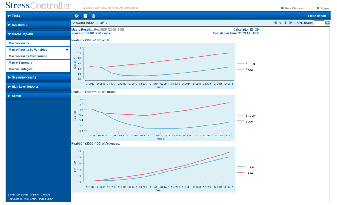
Stress ControllerTM produces time paths of macroeconomic variables such as those shown in Figure 3. These time series are the mean values of the variables in question conditional on the assumed shocks to the scenario variables. Note that, as an alternative to generating macroeconomic scenarios within Stress ControllerTM one may import a scenario in the form of a set of time series for different macroeconomic variables. Hence, one may work with scenarios generated by regulators or a bank economics department, importing the scenario time series into the application and then performing additional calculations with them.
Figure 1: The Stress ControllerTM Web Application
Figure 2: Editing Scenarios - Shocks to GDP
3. The AUM of the Asset Manager
The current size of AUM for the asset manager in this case study is around £106 billion, about 40 times the asset manager‟s total assets and about 80 times the total shareholders‟ equity. Breakdowns of the region- and asset-class-weights for the current AUM are displayed in Table 1.
| AUM class/weight by | ||||
|---|---|---|---|---|
| region UK | Europe | Asia | America | |
| Equity | 40% | 20% | 20% | 20% |
| Fixed Income | 40% | 20% | 20% | 20% |
| Multi Assets | 40% | 20% | 20% | 20% |
4. Modeling Financial Planning
In Figures 4 and 5, the historical consolidated summary financial statements of the asset manager are presented for the past 6 years. These historical financial statements, invented for the purpose of this exercise, are imported into Stress ControllerTM and serve as the starting point for forecasts of future financial statements conditional on macroeconomic scenarios.[1]
Figure 4: Historical Consolidated Statements of Financial Position and Assets under Management 2007 2008 2009 2010 2011 2012 As at 31 December £'000 £'000 £'000 £'000 £'000 £'000 Assets Cash, balances at central banks and items in the course of collection 822,771 741,238 794,683 872,990 952,274 1,036,715 Gross loans and advances to banks 80,336 95,510 82,366 75,694 94,982 81,878 Less: bank allowance for impairment 96 96 96 96 90 82 Loans and advances to banks 80,240 95,414 82,270 75,598 94,892 81,796 Gross loans and advances to customers 715,564 948,398 865,216 880,652 884,972 870,728 Less: customers allowance for impairment 24,768 24,768 24,768 24,768 21,104 19,270 Loans and advances to customers 690,796 923,630 840,448 855,884 863,868 851,458 Other assets 37,600 49,552 47,706 46,674 50,378 48,326 Total assets 1,631,407 1,809,834 1,765,107 1,851,146 1,961,412 2,018,295 Liabilities Deposits and items in the course of collection due to banks 184,676 233,090 155,824 158,592 184,170 157,166 Customer accounts 589,974 671,010 644,858 691,576 732,064 771,592 Other liabilities 37,870 36,408 34,124 31,410 33,044 33,174 Total liabilities 812,520 940,508 834,806 881,578 949,278 961,932 Shareholders equity Shareholders equity excluding noncontrolling interests 587,286 623,460 667,189 695,350 725,878 757,598 Noncontrolling interests 231,601 245,867 263,112 274,217 286,256 298,765 Total shareholders equity 818,887 869,326 930,301 969,568 1,012,134 1,056,363 Total liabilities and shareholders equity 1,631,407 1,809,834 1,765,107 1,851,146 1,961,412 2,018,295 Assets under management Total AUM 81,888,737 86,932,628 93,030,117 96,956,772 101,213,369 105,636,254 AUM equity 40,944,368 43,466,314 46,515,058 48,478,386 50,606,684 52,818,127 AUM fixed income 20,472,184 21,733,157 23,257,529 24,239,193 25,303,342 26,409,063 AUM multi asset 20,472,184 21,733,157 23,257,529 24,239,193 25,303,342 26,409,063
Figure 5: Historical Consolidated Income Statement 2007 2008 2009 2010 2011 2012 For the year ended 31 December £'000 £'000 £'000 £'000 £'000 £'000 Continuing operations Revenue 612,143 643,972 691,891 725,486 756,823 790,442 Net interest income 19,196 22,938 23,836 25,046 24,402 23,270 Total income 631,339 666,910 715,727 750,532 781,225 813,712 Credit impairment charges and other provisions (5,590) (5,590) (5,590) (5,590) (5,590) (5,590) Impairment of investment - - - - - - Operating expenses (280,522) (280,522) (280,522) (280,522) (280,522) (280,522) Other - - - - - - Profit before tax 345,227 380,798 429,615 464,420 495,113 527,600 Taxation (69,045) (76,160) (85,923) (92,884) (99,023) (105,520) Profit after tax from continuing operations 276,182 304,639 343,692 371,536 396,090 422,080 Profit for the year from discontinued operations, including gain on disposal - - - - - - Profit after tax 276,182 304,639 343,692 371,536 396,090 422,080
1The calculations are performed on a quarterly basis so the data is imported after converting the annual reports into quarterly data.
The key assumptions we make in modeling the asset manager‟s financial statements and capital planning are as follows:
1. We view the asset manager‟s financial and capital planning as Income Statement driven.
2. The Income Statement is modeled mainly via the following three components: (i) size and rate of the AUM (which will be described in detail below), (ii) growth of the expenses and (iii) the dividend payout. The latter two components can be calibrated by the user via parameters and can differentiate between different forecasting periods.
3. AUM forecasting The growth rate of each asset class is affected by (a) that asset class‟ historical performance and (b) the macroeconomic forecasts. The impact of the first element is calibrated by the user purely via time-series parameters. The impact of the second element is modeled as a weighted sum of sensitivity-adjusted regional macro variable growth rates, where the influencing macro variable is determined by scripting and the regional weight distributions and sensitivities to each regional macro-variable are calibrated via matrix type parameters. (Note that no time-series dimension is involved.)This is explained by the equations below:
AUMi,t+1 = AUMi,t(1 + Gi,t+1) R
Gi,t+1 = Pi,t+1 + (MGi,r,t+1Wi,rSi,r)
r=1 Here: i: the ith AUM asset class; r: the rth macro region where r=1,2,…R; Gi,t+1: the growth rate of the ith AUM asset class in period t+1; Pi,t+1: is a user defined adjustment to the growth rate of ith AUM asset class in period t+1; MG is a three-dimensional macro variable growth rate matrix in which the dimensions are (1) macro variables, (2) macro regions and (3) time horizon. MGi,r,t+1: the growth rate of the influencing macro variable from the rth region of the ith AUM asset class in period t+1; Wi,r: the regional weight of the ith AUM asset class in the rth regional element of the influencing macro variable, it is constant over time;. Si,r: the sensitivity of the ith AUM asset class to the rth regional element of the influencing macro variable, it is constant over time;
4. AUM user override As an alternative to the calculation above, the user can specify the growth rate for any asset class in any period, denoted GORi,t+1. This specification will override the above calculation. The comprehensive modeling of AUM size can be summarized as: If GORi,t+1does not equal -999; R
Gi,t+1 = Pi,t+1 + (MGi,r,t+1Wi,rSi,r)
r=1 Else; Gi,t+1 = GORi,t+1 End; AUMi,t+1 = AUMi,t(1 + Gi,t+1)
5. Loans and deposits are assumed to be linked to (a) GDP growth in the relevant region, and (b) their own historical trend. The relative importance of (a) and (b) and the sensitivity to macro shocks vary for different loans and deposits.
6. The credit impairment charge is calculated as the expected losses of loans and advances to retail and wholesale customers, taking into account the lagged impact of macroeconomic variables on provisions. (Recall that loans are modeled as diversified pool exposures.)
7. The financial position statement is affected, apart from loans and deposits, by retained earnings calculated from Income Statement forecasts.
8. To balance the financial position statement at the end of each forecasting period, we adjust the gap between forecast „Total Assets‟ and „Total Liabilities and Shareholder Equities‟, allowing this gap to be absorbed by multiple items employing user-defined weights.
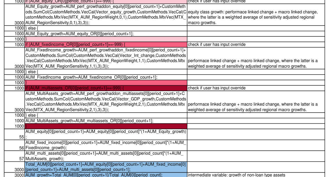
The equations for the financial statements analysis are treated in Stress ControllerTM as a part of the model‟s data. They are imported from a „feeder‟ Excel workbook. A screenshot of the equations stored in such a workbook is provided in Figure 6.
To take an example, the growth rate of the Fixed Income asset class of AUM is modeled as:
AUM_FixedIncome_growth=AUM_perf_growthaddon_fixedincome[0][period_count+1]+CustomMet hods.SumCol(CustomMethods.VecCal(Vector_Int_change,CustomMethods.VecCal(CustomMethods.M txVec(MTX_AUM_RegionWeight,1,1),CustomMethods.MtxVec(MTX_AUM_RegionSensitivity,1,1),3), 3));
Before the above equation is executed, all the variables employed in the equation must be declared by importing a user workbook containing the definition of each variable.
5. Modeling Pillar I Capital Planning
We model the Pillar I capital requirement and resources of the asset manager as follows:
1. Credit risk capital: 8% of the credit risk RWA. And the credit risk RWA is modeled as taking the trend of the provision results from the „ICAAP module‟ of Stress ControllerTM and applying it on the historical credit risk RWA.
2. Market risk capital: this is modeled as taking the trend of the forecasted total assets and applying it to the historical market risk required capital.
3. Operational risk capital: the standard approach is implemented, i.e. 12% of the forecasted revenue.
4. Pillar I capital resources are modelled in a simple manner in that Tier 1 capitals assumed to equal forecast shareholder equity. Tier 2 capital and the capital reduction are supposed to be constant over time.
6. Results
Using the approach described above, we performed an analysis of the impact of several stress scenarios on the asset manager‟s AUM and financial and capital planning. We present below results for (i) a base case (i.e., an unconditional forecast), (ii) a UK recession and (iii) a customer loss scenario.
The recession scenarios assume a sequence of shocks to real GDP in the geographical region in question. In all cases, the shocks are -2% in Q1, -1% in Q2 and -0.5% in Q3, Q4, Q5 and Q6. These shocks sum to a cumulative negative shock of 5% over 1.5 years. The customer loss scenario assumes a 3% decline in AUM in each quarter for the first 4 quarters. These shocks sum to a cumulative reduction in AUM of 12% over 1 year.
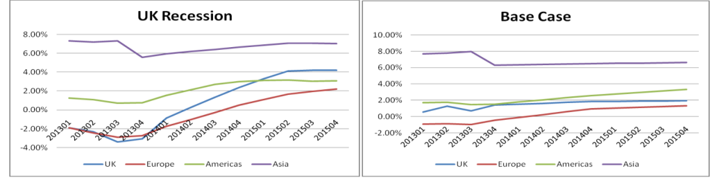
Figure 7 shows the effects of the base case and UK recession scenarios on GDP growth rates in different regions. Conditional on set of negative shocks to UK GDP, the model generates forecasts of all other macroeconomic variables including GDP in other regions and market prices including equity indices and interest rates by region. We perform the analysis from the perspective of information available at the end of 2012. Europe was still exhibiting a slight negative growth rate at that time which is then reflected in depressed growth in the first few periods of the projection.
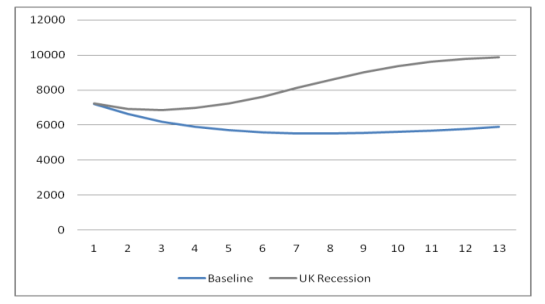
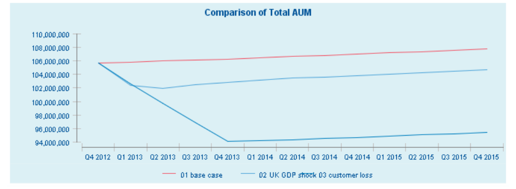
Within the model, the UK recession scenario has an impact on the ratings of the private bank‟s counter-parties and hence boosts credit impairment provisions as shown in Figure 8. This scenario also leads to a drop in equity indices with reduces AUM. The impact on is only partially compensated by a rise in the value of bond funds that occurs through lower interest rates. Figure 9 shows the forecast dynamics of AUM under the base case and the two scenarios of client loss and UK recession.
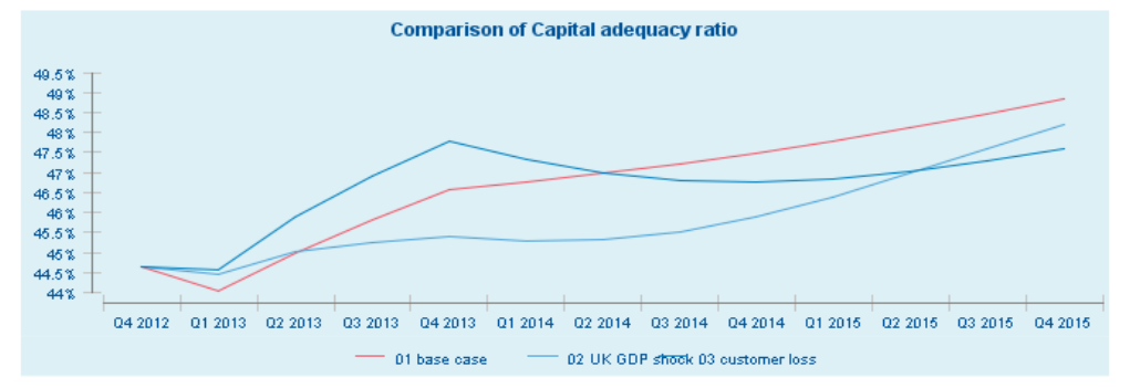
Figure 10 shows the impact of the scenarios on the asset manager‟s capital adequacy ratio. Customer loss leads to an immediate loss of revenue. This reduces capital requirements in the short run but subsequently generates a loss of income erodes which profitability. The plot therefore shows a short-term rise in the capital ratio followed by a relative decline to below the level of the base case projection.
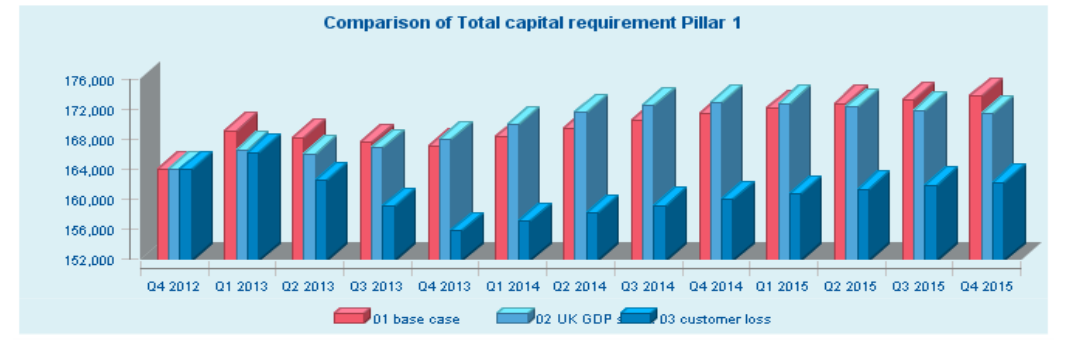
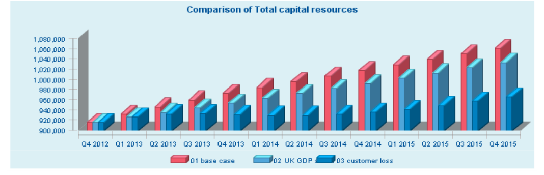
One may observe that the CAR ratio in the „03 customer loss‟ scenario remains higher than that of „01 base case‟ for the first 5 quarters. This is because the shock to AUM reduces revenue and hence the Pillar 1 operational risk capital required. This leads to a quasi-linear reduction in capital required (recall that the shock reduce in customer is about 12% for the first 4 quarters) whereas the capital available reduces at a much slower speed. Figures 11 and 12 show time paths of the numerator and denominator of the CAR ratio.
7. Conclusion
The analysis in this note is illustrative of how Stress ControllerTM may be used to perform stress testing of asset managers and private banks. It is straightforward to change the logic of the modelling to accommodate quite different forms of analysis. To illustrate, one may as an input to the calculations a central-case projection of the financial statements of an asset manager and model deviations from that base case as driven by shocks to market variables. Such an approach renders the analysis consistent with a set of forecasts generated by, for example, a Treasury function within an asset manager while permitting the risk function to investigate the impact on the business of a set of stress scenarios.
To this extent, Stress ControllerTM is an environment within which a wide range of company specific financial statement and capital projections may be performed.
Appendix
1.Controls
hist_len=24; print(period_count+1);
2. Macro variables
UK_GDP_current=CustomMethods.Exp(UK_GDP_log[0][period_count+1]); Europe_GDP_current=CustomMethods.Exp(Europe_GDP_log[0][period_count+1]); Americas_GDP_current=CustomMethods.Exp(Americas_GDP_log[0][period_count+1]); AfricaAndMiddleEast_GDP_current=CustomMethods.Exp(AfricaAndMiddleEast_GDP_log[0][period_count+ 1]); Asia_GDP_current=CustomMethods.Exp(Asia_GDP_log[0][period_count+1]); UK_Equity_current=CustomMethods.Exp(UK_Equity_log[0][period_count+1]); Europe_Equity_current=CustomMethods.Exp(Europe_Equity_log[0][period_count+1]); Americas_Equity_current=CustomMethods.Exp(Americas_Equity_log[0][period_count+1]); AfricaAndMiddleEast_Equity_current=CustomMethods.Exp(AfricaAndMiddleEast_Equity_log[0][period_cou nt+1]); Asia_Equity_current=CustomMethods.Exp(Asia_Equity_log[0][period_count+1]); UK_GDP_previous=CustomMethods.Exp(UK_GDP_log[0][period_count]); Europe_GDP_previous=CustomMethods.Exp(Europe_GDP_log[0][period_count]); Americas_GDP_previous=CustomMethods.Exp(Americas_GDP_log[0][period_count]); AfricaAndMiddleEast_GDP_previous=CustomMethods.Exp(AfricaAndMiddleEast_GDP_log[0][period_count ]); Asia_GDP_previous=CustomMethods.Exp(Asia_GDP_log[0][period_count]); UK_Equity_previous=CustomMethods.Exp(UK_Equity_log[0][period_count]); Europe_Equity_previous=CustomMethods.Exp(Europe_Equity_log[0][period_count]); Americas_Equity_previous=CustomMethods.Exp(Americas_Equity_log[0][period_count]); AfricaAndMiddleEast_Equity_previous=CustomMethods.Exp(AfricaAndMiddleEast_Equity_log[0][period_co unt]); Asia_Equity_previous=CustomMethods.Exp(Asia_Equity_log[0][period_count]);
3. BS model round 1
BS_Cash[0][period_count+1]=CustomMethods.MovAve(BS_Cash[0],period_count,8); Europe_CPI_growth=CustomMethods.Exp(Europe_CPI_log[0][period_count+1])/CustomMethods.Exp(Euro pe_CPI_log[0][period_count])-1; Americas_CPI_growth=CustomMethods.Exp(Americas_CPI_log[0][period_count+1])/CustomMethods.Exp(A mericas_CPI_log[0][period_count])-1; BS_LoanToBanks[0][period_count+1]=(Loan_TrendWeight[0][0]*CustomMethods.GrowAve(BS_LoanToBan ks[0], period_count, 8)+(1- Loan_TrendWeight[0][0])*(Loan_UK_Weight[0][0]*Loan_UK_SensitivityToGDP[0][0]*(UK_GDP_current/ UK_GDP_previous- 1)+Loan_Europe_Weight[0][0]*Loan_Europe_SensitivityToGDP[0][0]*(Europe_GDP_current/Europe_GDP _previous- 1)+Loan_Americas_Weight[0][0]*Loan_Americas_SensitivityToGDP[0][0]*(Americas_GDP_current/Americ as_GDP_previous- 1)+Loan_AfricaAndME_Weight[0][0]*Loan_AfricaAndME_SensitivityToGDP[0][0]*(AfricaAndMiddleEast_ GDP_current/AfricaAndMiddleEast_GDP_previous- 1)+Loan_Asia_Weight[0][0]*Loan_Asia_SensitivityToGDP[0][0]*(Asia_GDP_current/Asia_GDP_previous- 1))+1)*BS_LoanToBanks[0][period_count]*(1+Loan_SensitivityToCPI[0][0]*(Europe_CPI_growth+Americas _CPI_growth)/2); Credit_Pool_Provision[0][hist_len-4]=Credit_Pool_Provision[0][hist_len-1]; Credit_Pool_Provision[0][hist_len-3]=Credit_Pool_Provision[0][hist_len-1]; Credit_Pool_Provision[0][hist_len-2]=Credit_Pool_Provision[0][hist_len-1];
Ave_CreditPoolProvision_current=(Credit_Pool_Provision[0][period_count+1]+Credit_Pool_Provision[0][pe riod_count]+Credit_Pool_Provision[0][period_count-1]+Credit_Pool_Provision[0][period_count-2])/4.0; Ave_CreditPoolProvision_previous=(Credit_Pool_Provision[0][period_count]+Credit_Pool_Provision[0][per iod_count-1]+Credit_Pool_Provision[0][period_count-2]+Credit_Pool_Provision[0][period_count-3])/4.0; BS_LAToBanks_Scaling=BS_LoanToBanks[0][period_count+1]/BS_LoanToBanks[0][hist_len-1]; BS_Allowance_Banks[0][period_count+1]=BS_Allowance_Banks[0][period_count]+Ave_CreditPoolProvisio n_current*BS_LAToBanks_Scaling/4.0*Credit_Provision_FractionOfBank[0][period_count+1]- Loan_WriteOff_banks[0][period_count+1]*(Ave_CreditPoolProvision_current/Ave_CreditPoolProvision_pre vious); BS_NetLoanToBanks[0][period_count+1]=BS_LoanToBanks[0][period_count+1]- BS_Allowance_Banks[0][period_count+1]; BS_LoanToCustomers[0][period_count+1]=(Loan_TrendWeight[0][0]*CustomMethods.GrowAve(BS_LoanT oCustomers[0], period_count, 8)+(1- Loan_TrendWeight[0][0])*(Loan_UK_Weight[0][0]*Loan_UK_SensitivityToGDP[0][0]*(UK_GDP_current/ UK_GDP_previous- 1)+Loan_Europe_Weight[0][0]*Loan_Europe_SensitivityToGDP[0][0]*(Europe_GDP_current/Europe_GDP _previous- 1)+Loan_Americas_Weight[0][0]*Loan_Americas_SensitivityToGDP[0][0]*(Americas_GDP_current/Americ as_GDP_previous- 1)+Loan_AfricaAndME_Weight[0][0]*Loan_AfricaAndME_SensitivityToGDP[0][0]*(AfricaAndMiddleEast_ GDP_current/AfricaAndMiddleEast_GDP_previous- 1)+Loan_Asia_Weight[0][0]*Loan_Asia_SensitivityToGDP[0][0]*(Asia_GDP_current/Asia_GDP_previous- 1))+1)*BS_LoanToCustomers[0][period_count]*(1+Loan_SensitivityToCPI[0][0]*(Europe_CPI_growth+Ame ricas_CPI_growth)/2); BS_LAToCustomers_Scaling=BS_LoanToCustomers[0][period_count+1]/BS_LoanToCustomers[0][hist_len- 1]; BS_Allowance_Customers[0][period_count+1]=BS_Allowance_Customers[0][period_count]+BS_LAToCusto mers_Scaling*Ave_CreditPoolProvision_current/4.0*(1- Credit_Provision_FractionOfBank[0][period_count+1])- Loan_WriteOff_customers[0][period_count+1]*(Ave_CreditPoolProvision_current/Ave_CreditPoolProvision _previous); BS_NetLoanToCustomers[0][period_count+1]=BS_LoanToCustomers[0][period_count+1]- BS_Allowance_Customers[0][period_count+1]; BS_OtherAssets[0][period_count+1]=CustomMethods.MovAve(BS_OtherAssets[0],period_count,8); BS_TotalAssets[0][period_count+1]=BS_Cash[0][period_count+1]+BS_NetLoanToBanks[0][period_count+1 ]+BS_NetLoanToCustomers[0][period_count+1]+BS_OtherAssets[0][period_count+1]; BS_DueToBanks[0][period_count+1]=CustomMethods.MovAve(BS_DueToBanks[0],period_count,8)*(1+Dep osit_SensitivityToCPI[0][0]*(Europe_CPI_growth+Americas_CPI_growth)/2); BS_Deposits[0][period_count+1]=(Deposit_TrendWeight[0][0]*CustomMethods.GrowAve(BS_Deposits[0], period_count, 8)+(1- Deposit_TrendWeight[0][0])*(Loan_UK_Weight[0][0]*Deposit_UK_SensitivityToGDP[0][0]*(UK_GDP_cur rent/UK_GDP_previous- 1)+Loan_Europe_Weight[0][0]*Deposit_Europe_SensitivityToGDP[0][0]*(Europe_GDP_current/Europe_G DP_previous- 1)+Loan_Americas_Weight[0][0]*Deposit_Americas_SensitivityToGDP[0][0]*(Americas_GDP_current/Ame ricas_GDP_previous- 1)+Loan_AfricaAndME_Weight[0][0]*Deposit_AfricaAndME_SensitivityToGDP[0][0]*(AfricaAndMiddleEast _GDP_current/AfricaAndMiddleEast_GDP_previous- 1)+Loan_Asia_Weight[0][0]*Deposit_Asia_SensitivityToGDP[0][0]*(Asia_GDP_current/Asia_GDP_previou s- 1))+1)*BS_Deposits[0][period_count]*(1+Deposit_SensitivityToCPI[0][0]*(Europe_CPI_growth+Americas_C PI_growth)/2); BS_OtherLiabilities[0][period_count+1]=CustomMethods.MovAve(BS_OtherLiabilities[0],period_count,8);
BS_TotalLiabilities[0][period_count+1]=BS_DueToBanks[0][period_count+1]+BS_Deposits[0][period_count +1]+BS_OtherLiabilities[0][period_count+1]; UK_Int_Change=((UK_3MRate_log[0][period_count+1]- UK_3MRate_log[0][period_count])+(UK_10YRate_log[0][period_count+1]- UK_10YRate_log[0][period_count]))/2; Europe_Int_Change=((Europe_3MRate_log[0][period_count+1]- Europe_3MRate_log[0][period_count])+(Europe_10YRate_log[0][period_count+1]- Europe_10YRate_log[0][period_count]))/2; Americas_Int_Change=((Americas_3MRate_log[0][period_count+1]- Americas_3MRate_log[0][period_count])+(Americas_10YRate_log[0][period_count+1]- Americas_10YRate_log[0][period_count]))/2; AfricaAndMiddleEast_Int_Change=((AfricaAndMiddleEast_3MRate_log[0][period_count+1]- AfricaAndMiddleEast_3MRate_log[0][period_count])+(AfricaAndMiddleEast_10YRate_log[0][period_count +1]-AfricaAndMiddleEast_10YRate_log[0][period_count]))/2; Asia_Int_Change=((Asia_3MRate_log[0][period_count+1]- Asia_3MRate_log[0][period_count])+(Asia_10YRate_log[0][period_count+1]- Asia_10YRate_log[0][period_count]))/2; Average_Int_Change=Loan_UK_Weight[0][0]*UK_Int_Change+Loan_Europe_Weight[0][0]*Europe_Int_C hange+Loan_Americas_Weight[0][0]*Americas_Int_Change+Loan_AfricaAndME_Weight[0][0]*AfricaAnd MiddleEast_Int_Change+Loan_Asia_Weight[0][0]*Asia_Int_Change; LoanAsset_growth=(BS_LoanToBanks[0][period_count+1]+BS_LoanToCustomers[0][period_count+1])/(BS _LoanToBanks[0][period_count]+BS_LoanToCustomers[0][period_count]);
4. AUM model
UK_equity_growth=UK_Equity_current/UK_Equity_previous-1; Europe_equity_growth=Europe_Equity_current/Europe_Equity_previous-1; Asia_equity_growth=Asia_Equity_current/Asia_Equity_previous-1; Americas_equity_growth=Americas_Equity_current/Americas_Equity_previous-1; UK_GDP_growth=UK_GDP_current/UK_GDP_previous-1; Europe_GDP_growth=Europe_GDP_current/Europe_GDP_previous-1; Asia_GDP_growth=Asia_GDP_current/Asia_GDP_previous-1; Americas_GDP_growth=Americas_GDP_current/Americas_GDP_previous-1; double [] Vector_equity_growth = new double [] {UK_equity_growth, Europe_equity_growth, Asia_equity_growth, Americas_equity_growth}; double [] Vector_GDP_growth = new double [] {UK_GDP_growth, Europe_GDP_growth, Asia_GDP_growth, Americas_GDP_growth}; double [] Vector_Int_change = new double [] {UK_Int_Change, Europe_Int_Change, Asia_Int_Change, Americas_Int_Change}; print(82); print(MTX_AUM_Performance[1][1]); if (AUM_equity_OR[0][period_count+1]==-999) { AUM_Equity_growth=AUM_perf_growthaddon_equity[0][period_count+1]+CustomMethods.SumCol(Custo mMethods.VecCal(Vector_equity_growth,CustomMethods.VecCal(CustomMethods.MtxVec(MTX_AUM_Regi onWeight,0,1),CustomMethods.MtxVec(MTX_AUM_RegionSensitivity,0,1),3),3)); } else { AUM_Equity_growth=AUM_equity_OR[0][period_count+1]; } if (AUM_fixedincome_OR[0][period_count+1]==-999) { AUM_FixedIncome_growth=AUM_perf_growthaddon_fixedincome[0][period_count+1]+CustomMethods.Su mCol(CustomMethods.VecCal(Vector_Int_change,CustomMethods.VecCal(CustomMethods.MtxVec(MTX_AU M_RegionWeight,1,1),CustomMethods.MtxVec(MTX_AUM_RegionSensitivity,1,1),3),3)); } else { AUM_FixedIncome_growth=AUM_fixedincome_OR[0][period_count+1]; } if (AUM_multiassets_OR[0][period_count+1]==-999) { AUM_MultiAssets_growth=AUM_perf_growthaddon_multiassets[0][period_count+1]+CustomMethods.Sum Col(CustomMethods.VecCal(Vector_GDP_growth,CustomMethods.VecCal(CustomMethods.MtxVec(MTX_AU M_RegionWeight,2,1),CustomMethods.MtxVec(MTX_AUM_RegionSensitivity,2,1),3),3)); } else { AUM_MultiAssets_growth=AUM_multiassets_OR[0][period_count+1]; } AUM_equity[0][period_count+1]=AUM_equity[0][period_count]*(1+AUM_Equity_growth); AUM_fixed_income[0][period_count+1]=AUM_fixed_income[0][period_count]*(1+AUM_FixedIncome_gro wth); AUM_multi_assets[0][period_count+1]=AUM_multi_assets[0][period_count]*(1+AUM_MultiAssets_growth ); Total_AUM[0][period_count+1]=AUM_equity[0][period_count+1]+AUM_fixed_income[0][period_count+1] +AUM_multi_assets[0][period_count+1]; AUM_growth=Total_AUM[0][period_count+1]/Total_AUM[0][period_count];
5. IS model
IS_Revenue[0][period_count+1]=IS_Revenue[0][period_count]*AUM_growth; IS_Revenue[0][period_count+1]=IS_Revenue[0][period_count]*(AUM_growth+AUM_rate_growth_Addon[ 0][period_count+1]); IS_Revenue[0][period_count+1]=(AUM_equity[0][period_count+1]*AUM_equity_rate_bps[0][period_count +1]/10000+AUM_fixed_income[0][period_count+1]*AUM_fixedincome_rate_bps[0][period_count+1]/1000 0+AUM_multi_assets[0][period_count+1]*AUM_multiassets_rate_bps[0][period_count+1]/10000)/4.0; IS_NetIntIncome[0][period_count+1]=IS_NetIntIncome[0][period_count]*(IntIncome_Weight_On_Loan[0] [0]*LoanAsset_growth)*(1+IntIncome_Sensitivity_IntRate[0][0]*Average_Int_Change); IS_TotalIncome[0][period_count+1]=IS_Revenue[0][period_count+1]+IS_NetIntIncome[0][period_count+1 ]; BS_LATotal_Scaling=(BS_LoanToCustomers[0][period_count+1]+BS_LoanToBanks[0][period_count+1])/(B S_LoanToCustomers[0][hist_len-1]+BS_LoanToBanks[0][hist_len-1]); Provision_Charge_Ratio=-IS_CreditCharges[0][hist_len-1]*4.0/Credit_Pool_Provision[0][hist_len-1]; print(115); print(Credit_Pool_Provision[0][hist_len-1]); IS_CreditCharges[0][period_count+1]=- 1*BS_LATotal_Scaling*Provision_Charge_Ratio*Ave_CreditPoolProvision_current/4.0; print(2801); print(BS_LATotal_Scaling); print(2802); print(Ave_CreditPoolProvision_current); IS_ExtroImpairment[0][period_count+1]=Extrodinary_Impairment[0][period_count+1]; IS_OPExpenses[0][period_count+1]=IS_OPExpenses[0][period_count]*(1+OperationExpense_growth[0][per iod_count+1]); IS_OtherExpenses[0][period_count+1]=CustomMethods.MovAve(IS_OtherExpenses[0],period_count,8); IS_PBT[0][period_count+1]=IS_TotalIncome[0][period_count+1]+IS_CreditCharges[0][period_count+1]+IS _ExtroImpairment[0][period_count+1]+IS_OPExpenses[0][period_count+1]+IS_OtherExpenses[0][period_c ount+1]; IS_Tax[0][period_count+1]=- 1*CustomMethods.Max(0,1*Tax_AverageRate[0][0]*IS_PBT[0][period_count+1]); IS_PAT_ConOperation[0][period_count+1]=IS_PBT[0][period_count+1]+IS_Tax[0][period_count+1]; IS_DisconOperation[0][period_count+1]=Discontinued_GainLoss[0][period_count+1]; IS_PAT[0][period_count+1]=IS_PAT_ConOperation[0][period_count+1]- IS_DisconOperation[0][period_count+1];
6. BS model round 2
test1=CustomMethods.MovAve(IS_PAT[0], period_count,8); print(Dividend_Payout_Ratio[0][period_count+1]); Dividend=CustomMethods.Max(0, CustomMethods.MovAve(IS_PAT[0], period_count,8)*Dividend_Payout_Ratio[0][period_count+1]);
BS_Equity_Control[0][period_count+1]=BS_Equity_Control[0][period_count]+Capital_Injection[0][period_ count+1]+(IS_PAT[0][period_count+1]-Dividend); BS_Equity_NoControl[0][period_count+1]=BS_Equity_NoControl[0][period_count]; BS_TotalEquity[0][period_count+1]=BS_Equity_Control[0][period_count+1]+BS_Equity_NoControl[0][peri od_count+1]; BS_TotalLiaAndEquity[0][period_count+1]=BS_TotalLiabilities[0][period_count+1]+BS_TotalEquity[0][peri od_count+1]; BS_Cash[0][period_count+1]=CustomMethods.Max(0, BS_Cash[0][period_count+1]- CustomMethods.Max(IS_PAT[0][period_count+1],0)*Dividend_Payout_Ratio[0][period_count+1]); BS_TotalAssets[0][period_count+1]=BS_Cash[0][period_count+1]+BS_NetLoanToBanks[0][period_count+1 ]+BS_NetLoanToCustomers[0][period_count+1]+BS_OtherAssets[0][period_count+1];
7. BS re-balancing
BS_Cash[0][period_count+1]=BS_Cash[0][period_count+1]+CustomMethods.Max(0,BS_TotalLiaAndEquity[ 0][period_count+1]-BS_TotalAssets[0][period_count+1])*GapAbsorb_Asset_Cash[0][0]; BS_TradingAssets[0][period_count+1]=BS_TradingAssets[0][period_count+1]+CustomMethods.Max(0,BS_T otalLiaAndEquity[0][period_count+1]- BS_TotalAssets[0][period_count+1])*GapAbsorb_Asset_TradingPortfolio[0][0]; BS_OtherAssets[0][period_count+1]=BS_OtherAssets[0][period_count+1]+CustomMethods.Max(0,BS_Total LiaAndEquity[0][period_count+1]-BS_TotalAssets[0][period_count+1])*GapAbsorb_Asset_Other[0][0]; BS_DueToBanks[0][period_count+1]=BS_DueToBanks[0][period_count+1]+CustomMethods.Max(0,BS_Tot alAssets[0][period_count+1]- BS_TotalLiaAndEquity[0][period_count+1])*GapAbsorb_Liability_DueToBanks[0][0]; BS_Deposits[0][period_count+1]=BS_Deposits[0][period_count+1]+CustomMethods.Max(0,BS_TotalAssets[ 0][period_count+1]- BS_TotalLiaAndEquity[0][period_count+1])*GapAbsorb_Liability_CustomerAccount[0][0]; BS_DebtIssue[0][period_count+1]=BS_DebtIssue[0][period_count+1]+CustomMethods.Max(0,BS_TotalAsse ts[0][period_count+1]-BS_TotalLiaAndEquity[0][period_count+1])*GapAbsorb_Liability_DebtIssue[0][0]; BS_OtherLiabilities[0][period_count+1]=BS_OtherLiabilities[0][period_count+1]+CustomMethods.Max(0,BS _TotalAssets[0][period_count+1]- BS_TotalLiaAndEquity[0][period_count+1])*GapAbsorb_Liability_Other[0][0]; BS_TotalAssets[0][period_count+1]=BS_Cash[0][period_count+1]+BS_NetLoanToBanks[0][period_count+1 ]+BS_NetLoanToCustomers[0][period_count+1]+BS_OtherAssets[0][period_count+1]; BS_TotalLiabilities[0][period_count+1]=BS_DueToBanks[0][period_count+1]+BS_Deposits[0][period_count +1]+BS_OtherLiabilities[0][period_count+1]; BS_TotalLiaAndEquity[0][period_count+1]=BS_TotalLiabilities[0][period_count+1]+BS_TotalEquity[0][peri od_count+1]; BS_Gap_Check[0][period_count+1]=BS_TotalAssets[0][period_count+1]- BS_TotalLiaAndEquity[0][period_count+1];
8. Report items
Q0_Credit_RWA=RWA_CreditRisk[0][hist_len-1]; Q0_CreditPool_RWAProvision=Credit_Pool_RWAProvision[0][hist_len-1]; Credit_Pool_RWAProvision[0][hist_len-4]=Credit_Pool_RWAProvision[0][hist_len-1]; Credit_Pool_RWAProvision[0][hist_len-3]=Credit_Pool_RWAProvision[0][hist_len-1]; Credit_Pool_RWAProvision[0][hist_len-2]=Credit_Pool_RWAProvision[0][hist_len-1]; Ave_CreditPoolRWAProvision_current=(Credit_Pool_RWAProvision[0][period_count+1]+Credit_Pool_RWA Provision[0][period_count]+Credit_Pool_RWAProvision[0][period_count- 1]+Credit_Pool_RWAProvision[0][period_count-2])/4.0; Ave_CreditPoolRWAProvision_previous=(Credit_Pool_RWAProvision[0][period_count]+Credit_Pool_RWA Provision[0][period_count-1]+Credit_Pool_RWAProvision[0][period_count- 2]+Credit_Pool_RWAProvision[0][period_count-3])/4.0; print(161); print(Ave_CreditPoolRWAProvision_previous);print(Ave_CreditPoolRWAProvision_current);
RWA_CreditRisk[0][period_count+1]=Q0_Credit_RWA*Ave_CreditPoolRWAProvision_current/Q0_CreditP ool_RWAProvision*BS_LATotal_Scaling; RWA_MarketRisk[0][period_count+1]=(BS_TradingAssets[0][period_count+1]+BS_FVAssets[0][period_cou nt+1]+BS_DerivativeAssets[0][period_count+1]+BS_ForSaleAssets[0][period_count+1])*MktRWA_MVAsset s_Ratio[0][period_count+1]*(Ave_CreditPoolRWAProvision_current/Ave_CreditPoolRWAProvision_previou s); RWA_MarketRisk[0][period_count+1]=RWA_MarketRisk[0][period_count]*(RWA_CreditRisk[0][period_co unt+1]/RWA_CreditRisk[0][period_count]); RWA_OperationalRisk[0][period_count+1]=BS_TotalAssets[0][period_count+1]*OpRWA_TotalAssets_Ratio [0][period_count+1]*(Ave_CreditPoolRWAProvision_current/Ave_CreditPoolRWAProvision_previous); RWA_Total[0][period_count+1]=RWA_CreditRisk[0][period_count+1]+RWA_MarketRisk[0][period_count+ 1]+RWA_OperationalRisk[0][period_count+1]; CoreTier1_Cap[0][period_count+1]=BS_TotalEquity[0][period_count+1]*CoreTier1_Equity_Ratio[0][period _count+1]; Tier1_Cap[0][period_count+1]=BS_TotalEquity[0][period_count+1]*Tier1_Equity_Ratio[0][period_count+1] ; Tier2_Cap[0][period_count+1]=BS_SubDebt[0][period_count+1]*Tier2_SubLiabilities_Ratio[0][period_cou nt+1]; Deduction_Cap[0][period_count+1]=(Tier1_Cap[0][period_count+1]+Tier2_Cap[0][period_count+1])*Deduc tion_Capital_Ratio[0][period_count+1]; Total_Cap[0][period_count+1]=Tier1_Cap[0][period_count+1]+Tier2_Cap[0][period_count+1]+Deduction_ Cap[0][period_count+1]; CoreTier1_CapRatio[0][period_count+1]=CoreTier1_Cap[0][period_count+1]/RWA_Total[0][period_count+ 1]; Tier1_CapRatio[0][period_count+1]=Tier1_Cap[0][period_count+1]/RWA_Total[0][period_count+1]; Total_CapRatio[0][period_count+1]=Total_Cap[0][period_count+1]/RWA_Total[0][period_count+1]; Return_On_Equity[0][period_count+1]=4.0*IS_PAT[0][period_count+1]/BS_Equity_Control[0][period_cou nt+1]; Return_On_RWA[0][period_count+1]=4.0*IS_PAT[0][period_count+1]/RWA_Total[0][period_count+1]; Loan_LossRate[0][period_count+1]=- 4.0*10000*IS_CreditCharges[0][period_count+1]/(BS_LoanToBanks[0][period_count+1]+BS_LoanToCusto mers[0][period_count+1]); Credit_RWA=(CapRequired_CreditRisk[0][hist_len- 1]/0.08)*Ave_CreditPoolRWAProvision_current/Q0_CreditPool_RWAProvision*BS_LATotal_Scaling; Credit_RWA=(CapRequired_CreditRisk[0][hist_len- 1]/0.08)*Ave_CreditPoolRWAProvision_current/Q0_CreditPool_RWAProvision; Credit_RWA=(CapRequired_CreditRisk[0][hist_len- 1]/0.08)*Ave_CreditPoolProvision_current/Ave_CreditPoolProvision_previous; CapRequired_CreditRisk[0][period_count+1]=Credit_RWA*0.08; CapRequired_MarketRisk[0][period_count+1]=CapRequired_MarketRisk[0][period_count]*(BS_TotalAssets [0][period_count+1]/BS_TotalAssets[0][period_count]); CapRequired_OperationalRisk[0][period_count+1]=IS_Revenue[0][period_count+1]*4*0.12; CapRequired_Total[0][period_count+1]=CapRequired_CreditRisk[0][period_count+1]+CapRequired_Market Risk[0][period_count+1]+CapRequired_OperationalRisk[0][period_count+1]; CapResources_Tier1[0][period_count+1]=CapResources_Tier1[0][period_count]+(BS_TotalEquity[0][period _count+1]-BS_TotalEquity[0][period_count]); CapResources_Tier2[0][period_count+1]=CapResources_Tier2[0][period_count]; CapResources_Deduction[0][period_count+1]=CapResources_Deduction[0][period_count]; CapResources_Total[0][period_count+1]=CapResources_Tier1[0][period_count+1]+CapResources_Tier2[0][ period_count+1]+CapResources_Deduction[0][period_count+1]; CapRatio_Adequacy[0][period_count+1]=CustomMethods.ConvertNaNAndInfinite(CapResources_Total[0][p eriod_count+1]/CapRequired_Total[0][period_count+1],0);
Risk Control Limited 13-14 Dean Street London W1D 3RS +44(0)2033070730 www.riskcontrollimited.com