

1. Introduction
A common challenge for banks is to develop consistent scenarios suitable for use as inputs to their regulatory or internal stress testing programmes. Regulators or senior managers may suggest scenarios involving certain variables but these rarely constitute a full of set of economic risk drivers for the bank’s loan book and other portfolios. The risk or the economics department of the bank is then faced with the task of “expanding the scenario”, i.e., coming up with plausible values for the key risk drivers not included in the original stress test specification.
To take an example, a bank’s board might ask how it would be affected by a US recession. Clearly, such a recession would affect GDP in other regions and would also have an impact on market variables such as equity indices, interest rates, currency values and commodity and property prices. Attributing values to these other variables, before analysing the impact on credit and market exposures, is a difficult task.
As another instance, supervisors may require banks to perform stress tests as part of a coordinated program, evaluating multiple institutions in a coordinated manner. Such programs (for example, the EBA stress testing exercises in Europe or the CCAR in the United States) typically specify time paths for several variables but many other variables, are important for banks’ portfolios, are omitted from the specification.
While it is possible to “expand” a scenario to include other variables by exercising judgment (and this approach is common in banks), there are significant advantages to use of more data-driven and semi-automatic techniques. Especially for risk exercises that generate regulatory data, such as regulatory capital or stress testing, supervisory authorities commonly prefer risk processes that leave little to the discretion of the banks involved.
To meet the needs of banks involved in stress testing, RCL has developed a data-driven framework for consistent scenario expansion. The approach utilises a statistical macroeconomic model to calculate conditional means of a set of variables given prescribed values for others. The procedure substantially reduces the need for users to utilise expert judgement, leading to greater objectivity and consistency. This note describes the approach in broad terms and provides a step-by-step case study of its application.
The approach is delivered using RCL’s Stress ControllerTM software. This software is a Java Enterprise web application which may be installed on a client’s own internal servers. Users then interact flexibly with the software using browsers. (Alternatively, an instance of the software may be hosted on the client’s behalf by RCL on its own secure servers.) The software permits one to create, store and manipulate scenarios specified in terms of macroeconomic variables.
The software provides a highly secure environment suitable for analysis aimed at generating regulatory reports for supervisors. All calculations are stored in a relational database and are available for subsequent audit. User roles and actions are tightly controlled. The software is a mature application that is licensed to major banks and asset managers and to several central banking institutions.
2. The Case Study
To “fill in” variables or “expand” the scenario, our approach makes use of a multi-region, statistical macroeconomic model. This model consists of a time-series forecasting-model for vectors of macroeconomic variables in multiple geographical regions.
For each country-region, a set of macroeconomic variables is modelled as a first order Vector Autoregression. A set of global variables such as commodity process is also modelled. Weighted averages of variables from other regions and global variables affect the vector of variables corresponding to each country-region. This framework permits the user to model the evolution of key macroeconomic variables in each country-region in a flexible manner while including feedback or “contagion” between countries.
The basic approach resembles that of Pesaran, Shuermann and Weiner (2002). However, we endogenise global variables such as the oil or gold prices. The model is an example of the Global Vector Autoregressive (GVAR) models.[1] These models have been used in stress testing by central banks and regulators. For example, the Oesterreichische Nationalbank uses a variant of the GVAR approach in generating and analysing scenarios in the context of stress testing.
To illustrate the approach, in this note, we provide a case study, expanding scenarios to include conditional forecasts of additional risk drivers. The dataset that we are interested in estimating in this note consists of the regions/countries and variables summarised in Table 1.
The scenarios we examine are the “baseline” and “adverse” macroeconomic scenarios developed by the European Systemic Risk Board and employed in stress testing by the European Banking Authority (EBA). These consist of assumptions about future GDP growth and Consumer Price Inflation for several countries as displayed in Tables 2 and 3 below.
1 See Pesaran, Shuermann and Weiner (2002), Dees, Di Mauro, Pesaran, and Smith (2005) and Dees, Holly, Pesaran and Smith (2007).
The task to be completed, therefore, is to produce forecasts of the variables which appear in Table 1 conditional on the variables that appear in Tables 2 and 3.
First, we convert the growth rates in the scenario into levels so they can be used as inputs to Stress ControllerTM. Second, we interpolate the scenario data (using cubic splines) so as to obtain a “quarterly data version” of the scenario. We do this for convenience since Stress ControllerTM is generally run with quarterly data, although other data frequencies may be employed. The resulting quarterly data is shown in Table 4.
Scenario data may be loaded into Stress ControllerTM either via an input file or through entering information through the graphical user interface. To employ the first of these approaches, the user creates a worksheet entitled “Default-Macro Base Overrides” in the “Default_values.xls” workbook. Once loaded, the data appears in the interface as shown in Figure 1.
After feeding scenario data into Stress ControllerTM, it is straightforward to expand the scenario to other macroeconomic time series. The model calculates period-by-period, conditional means of variables not among the prescribed scenario variables, given the specified values of the scenario variables, and given the values that all the variables took in the previous period.
Figure 1: Scenario Data Viewed through the Interface
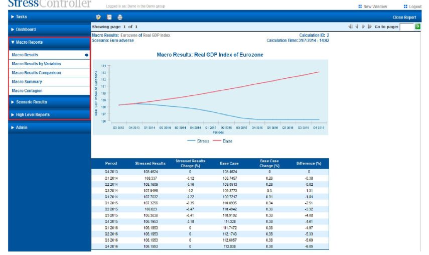
Results from the calculations may be exported from Stress Controller for further analysis or displayed through reports that appear in the Stress ControllerTM interface. These reports typically exhibit a base and a stress case. Stress ControllerTM may be configured to yield:
| USA | Italy | France | Japan | Eurozone | Asia | Spain | Po rtugal | |
|---|---|---|---|---|---|---|---|---|
| CPI | ✓ | ✓ | ✓ | ✓ | ✓ | ✓ | ✓ | ✓ |
| Real GDP (2005=100) | ✓ | ✓ | ✓ | ✓ | ✓ | ✓ | ✓ | ✓ |
| Debt to GDP Ratio | ✓ | ✓ | ✓ | ✓ | ✓ | ✓ | ✓ | ✓ |
| Equity Index | ✓ | ✓ | ✓ | ✓ | ✓ | ✓ | ✓ | ✓ |
| FX rate | ✓ | ✓ | ✓ | |||||
| 3-month Treasury Bill Rate | ✓ | ✓ | ✓ | ✓ | ||||
| 10-year Government Benchmark Rate | ✓ | ✓ | ✓ | ✓ |
| GDP Growth (%) | Inflation (%) | |||||||||
|---|---|---|---|---|---|---|---|---|---|---|
| 2014 | 2015 | 2016 6 | 2014 | 2015 | ||||||
| Spain 1.0 | 1.7 | 2.2 | 0.3 | 0.9 | ||||||
| France 1.0 | 1.7 | 2.3 | 1.2 | 1.2 | ||||||
| Italy 0.5 | 1.2 | 1.3 | 0.9 | 1.3 | ||||||
| Portugal 0.8 | 1.5 | 1.7 | 0.8 | 1.2 | ||||||
| Eurozone 1.2 | 1.8 | 1.7 | 1.0 | 1.3 |
| GDP Growth (%) | Inflation (%) | |||||||||
|---|---|---|---|---|---|---|---|---|---|---|
| 2014 | 2015 | 2016 6 | 2014 | 2015 | ||||||
| -0.3 | -1.0 | 0.1 | 0.3 | 0.4 | ||||||
| -0.4 | -1.1 | 0.4 | 1.1 | 0.7 | ||||||
| -0.9 | -1.6 | -0.7 | 0.9 | 1.0 | ||||||
| -0.8 | -2.3 | -1.1 | 0.7 | 0.1 | ||||||
| -0.7 | -1.4 | 0.0 | 1.0 | 0.6 |
| 2013 | 2014 | 2014 | 2014 | 2014 | 2015 | 2015 | 2015 | 2015 | 2016 | 2016 | 2016 | 2016 | |||
|---|---|---|---|---|---|---|---|---|---|---|---|---|---|---|---|
| 04 | 01 | 02 | 03 | 04 | 01 | 02 | 03 | 04 | 01 | 02 | 03 | 04 | |||
| Italy | CPI | 117.9 | 118.1 | 118.4 | 118.6 | 118.9 | 119.2 | 119.5 | 119.9 | 120.1 | 120.3 | 120.5 | 120.7 | 120.8 | |
| Real | GDP | 94.9 | 94.8 | 94.6 | 94.3 | 94.1 | 93.7 | 93.3 | 92.9 | 92.6 | 92.4 | 92.2 | 92.0 | 91.9 | |
| France | CPI | 113.4 | 113.7 | 114.1 | 114.4 | 114.6 | 114.9 | 115.1 | 115.3 | 115.4 | 115.4 | 115.4 | 115.3 | 115.1 | |
| Real | GDP | 106.1 | 106.0 | 105.9 | 105.8 | 105.6 | 105.4 | 105.0 | 104.6 | 104.5 | 104.5 | 104.5 | 104.7 | 104.9 | |
| Eurozone | CPI | 117.1 | 117.4 | 117.7 | 118.0 | 118.2 | 118.5 | 118.6 | 118.8 | 119.0 | 119.1 | 119.2 | 119.3 | 119.3 | |
| Real | GDP | 108.5 | 108.3 | 108.2 | 107.9 | 107.7 | 107.3 | 106.8 | 106.4 | 106.2 | 106.2 | 106.2 | 106.2 | 106.2 | |
| Spain | CPI | 121.1 | 121.2 | 121.3 | 121.4 | 121.5 | 121.6 | 121.7 | 121.8 | 122.0 | 122.2 | 122.4 | 122.7 | 123.0 | |
| Real | GDP | 101.5 | 101.5 | 101.4 | 101.3 | 101.2 | 101.0 | 100.6 | 100.3 | 100.2 | 100.2 | 100.2 | 100.2 | 100.3 | |
| Portugal | CPI | 116.4 | 116.7 | 116.9 | 117.1 | 117.2 | 117.3 | 117.3 | 117.3 | 117.3 | 117.3 | 117.1 | 116.8 | 116.5 | |
| Real | GDP | 97.7 | 97.6 | 97.5 | 97.2 | 96.9 | 96.5 | 95.8 | 95.2 | 94.7 | 94.4 | 94.1 | 93.8 | 93.7 |
Note: Real GDP is indexed at 2005 levels.
1. A base case equal to an expanded version of a given base scenario and
2. A stress case equal to an expanded version of a stress scenario.
Figures 2 and 3 provide screen shots of example reports calculated for the EBA Base and Adverse macroeconomic scenarios. A variety of other reports is available through the interface.
Figure 3: Example Macro Summary Report
It is straightforward to export data from the reports into formats including Microsoft Excel, Word or Powerpoint. Alternatively, one may use a separate export facility which produces Excel workbooks in a prescribed format.
3. Results
In this section, we examine the results of our scenario expansion exercise using the variables and regions described in the last section and the scenarios specified in Tables 2 and 3.
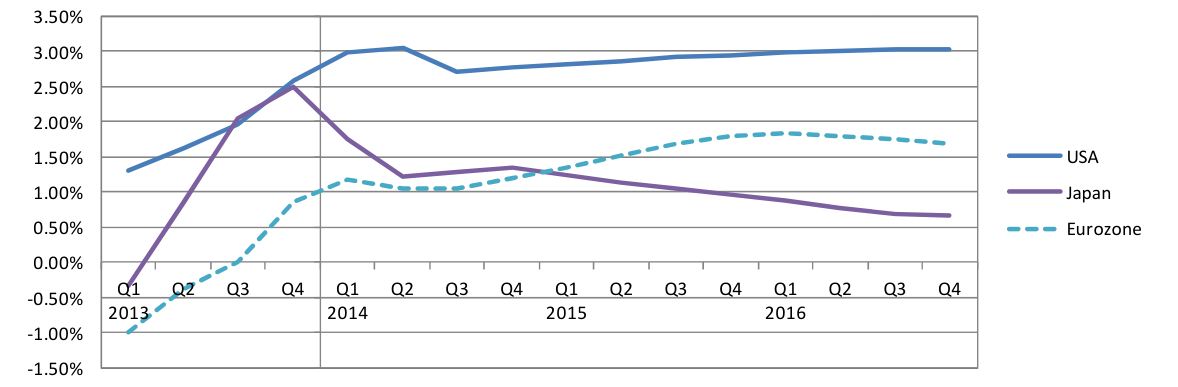
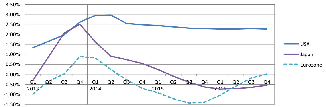
Figures 4 and 5 show the impact of our two scenarios on Japanese and US GDP. Eurozone GDP growth declines from between 1 and 2% in the period from 2014 to 2016 in our base scenario to consistently negative growth (almost reaching -1.5% at one point) in the adverse scenario. Note that while the time paths of Eurozone GDP (indicated in both figures by the dotted line) have already been specified as part of the scenarios, the paths of US and Japanese GDP have not. We generate consistent Japanese and US growth forecasts; the forecasts in the figures below are, thus, conditional forecasts. In the base case, Japanese growth falls from around 2% to just above 0.5%. US growth is more or less constant, around 2%.
The Eurozone recession specified in the adverse scenario has the expected impact on both the Japanese and the US economies (although the magnitudes of the effects differ between the two countries). US growth falls from 3% to below 2.5% over the first couple of quarters although it is rebounding strongly by the end of the observed period. The effect on Japan is stronger; the Eurozone recession causes growth to fall steadily and by the end of the observed period Japanese GDP is shrinking, although it starts to rebound at the end of the forecasted period.
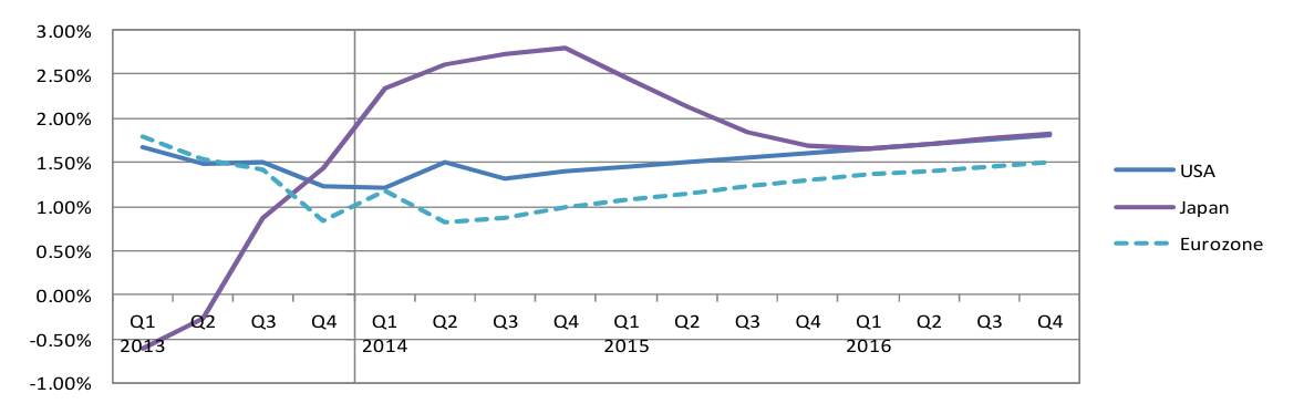
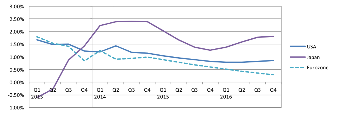
Figure 6 shows the time paths followed by Consumer Price Indices in the Eurozone, US and Japan in the EBA’s base scenarios. Figure 3 shows time paths for the same variables in the adverse scenario. Once again, Eurozone CPI growth rates have been specified as part of our scenario and are included for comparison.
US and Japanese CPIs behave as one might intuitively expect in the adverse scenario with the deflationary pressure in the adverse scenario feeding through into lower inflation rates in the US and Japan – this can be seen in Figure 7.
Stress ControllerTM is able to expand partial scenarios in two main ways. As described for GDP and CPI above, given forecasts of risk indicators in certain regions it may be used to generate consistent forecasts for the same risk indicators in other regions. Additionally, however, it may also be used to generate forecasts for risk indicating variables that are not specified anywhere as a part of a scenario, for instance, market variables, for example, in this case: equity indices, interest rates, and commodity prices.
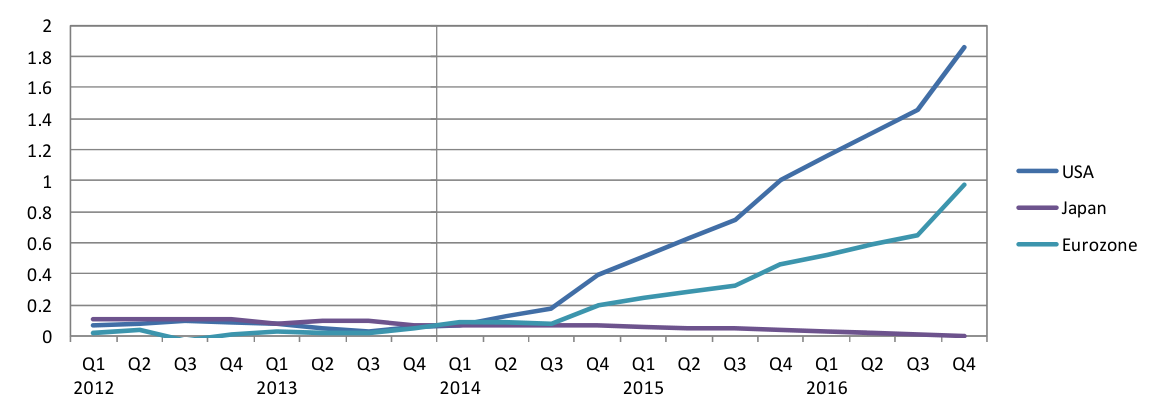
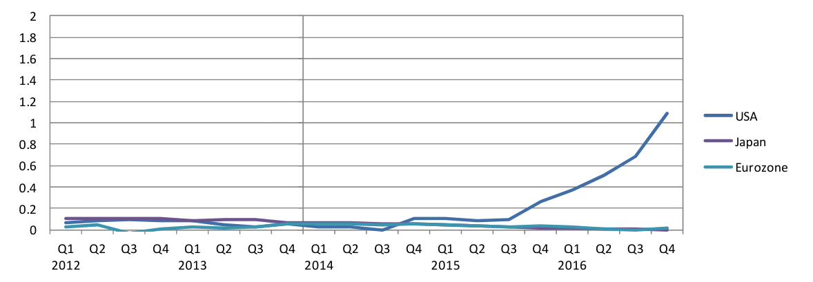
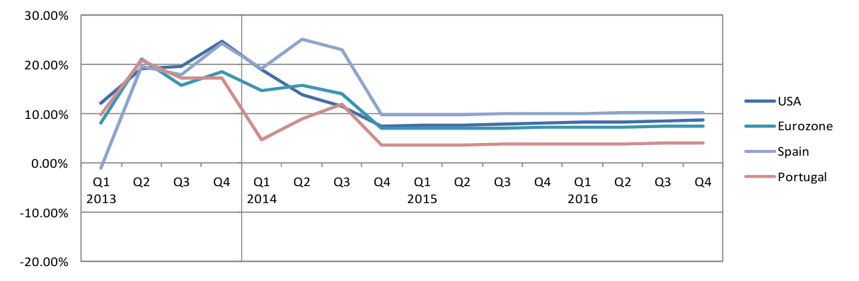
As part of this case study, we display, below illustrative results for 3-Month Treasury bill rates in the US, Eurozone, and Japan, as well as equity market indices for all our forecasted regions.
Figures 8 and 9 show the effect of our two EBA scenarios on 3-Month Treasury bill rates. Again, results are shown for the US, Japan and the Eurozone. Note that, in the graphs below, the Eurozone data are displayed as a line (instead of a dotted line). This is to indicate that interest rates in the Eurozone have not been specified as part of our two scenarios but are instead forecasted conditionally based on the specified CPI and GDP paths. As might be expected, both three-month-interest-rates data series are lower in the adverse scenario than in the base case.
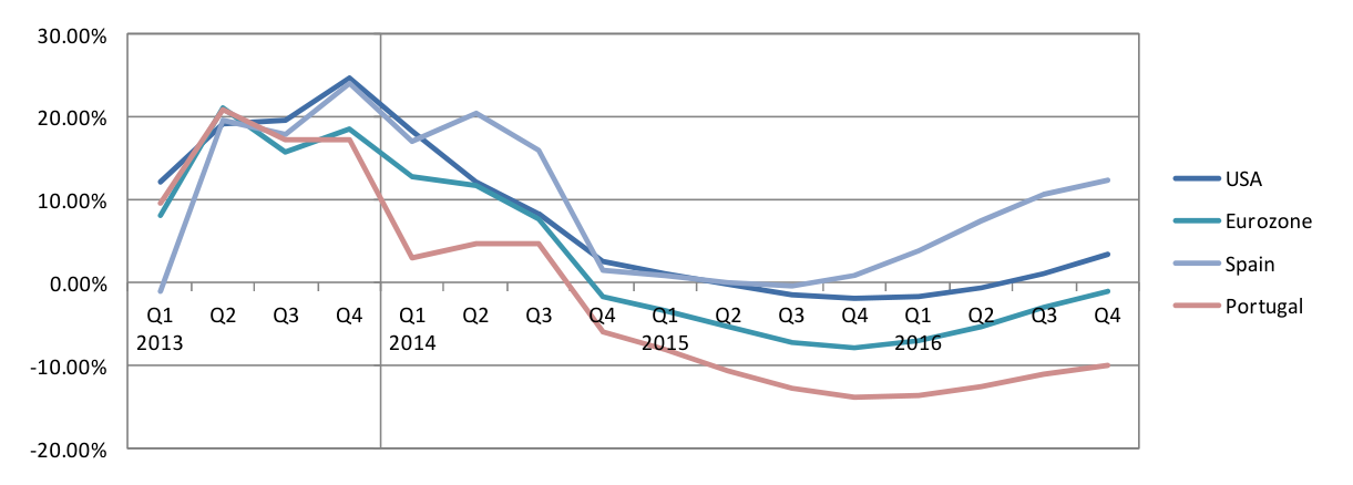
The model predictions for the behaviour of equity indices are shown below in Figures 10 and 11, this time for: the US, Spain, Portugal and the Eurozone. In the base case, equity indices for all the countries/regions are predicted to converge to different long run growth rates of between 4 - 10% In contrast, as Figure 11 shows, all countries’ indices growth rates fall steeply in the adverse scenario before recovering. As expected, equity indices’ growth rates appear much more volatile than GDP and CPI in our model.
Consistent Scenario Expansion-Case Study
References
Dées, Stéphane, Filippo di Mauro, Hashem Pesaran and Vanessa Smith (2005) “Exploring the international linkages of the euro area: a global VAR analysis,” Journal of Applied Econometrics, 22(1), January, pp. 1-38.
Dées, Stéphane, Sean Holly, Hashem Pesaran and Vanessa Smith (2007) “Long run macroeconomic relations in the global economy,” Economics, 1(3), May, pp. 1-20.
Pesaran, Hashem, Til Shuermann and S.M. Weiner (2002) “Modeling Regional Interdependencies using a Global Error-Correcting Macroeconometric Model,” Wharton School discussion paper 01-38-B.
Risk Control Limited 13-14 Dean Street London W1D 3RS UK T: +44 (0)203 307 0730 www.riskcontrollimited.com