Capital and Risk in Bancassurance Organisations

1 Introduction

This paper analyzes the risk and capital implications of creating financial conglomerates that combine banking and insurance. In Europe, the Second banking Directive of 1989 allowed banks to combine banking, insurance and other financial services under a single corporate structure. Similar deregulation took place in the US by means of Gramm-Leach-Bliley Act of 1999 which permitted US bank holding company (BHC) to operate as universal bank. These deregulations resulted in an expansion in financial conglomeration.

In the period since this deregulation, many banks have built up significant bancassurance operations. Bancassurance operations involve manufacturing and/or distributing insurance products in parallel to banking businesses. Distribution in this sense means either direct selling of insurance products through the bank’s branches or the bank acting as an agent for an insurer and promoting the insurer’s products to its clients. Following the recent crisis, banks with insurance operations are actively considering whether to divest themselves of non-core businesses including insurance operations in order to bolster their capital. Meanwhile, regulators are considering what should be the capital treatment of investments in other financial businesses including insurance.

The motives for a bank to engage in insurance activities are two fold. First, there may be synergies in the distribution of insurance products through the same network as a bank has established to sell retail banking services. Pooling information about a client may be helpful for selling both kinds of product while it may also be useful to the client to have a one-stop shop for both banking and insurance products. Second, returns on banking, insurance and other financial activities may be relatively uncorrelated and hence a bancassurer may be able to economize on capital by combining two such operations.

Numerous studies in the literature examine the impact of diversification on financial conglomerates including bancassurance. It remains controversial whether diversification provides tangible benefits either for individual firms or for financial market as a whole. Some studies, including Boyd, Graham, and Hewitt (1993), Carow (2001), Chen, Li, Liao, Moshirian, and Szablocs (2009), Chen and Tan (2011), emphasize economies of scope coupled and reductions in default probabilities due to low correlations in revenue streams. Other studies, including Hoyt and Trieschmann (1991), Allen and Jagtiani (2000), Amel, Barnes, Panetta, and Salleo (2004), Laeven and Levine (2007), De Jonghe

(2010) emphasize costs of diversification. On the latter, one may argue that investors can diversify away risk by constructing efficient portfolios rather than requiring conglomeration of diverse businesses. Furthermore, diversification within a single entity may intensify agency problems between corporate insiders and small shareholders with adverse implications for market values. Lastly, consolidation and internationalization may result in more concentrated financial market, which increases systemic risk.

Our study contributes to the above literature by quantifying the economies in capital that can be effected by diversifying across banking and insurance operations. We do not attempt to quantify other benefits such as those due to economies of scope (see, for example, Dreassi and Schneider (2015)), or costs such as those from influences on systemic risk (see Mhlnickel and Wei (2015) and Slijkerman, Schoenmaker, and de Vries (2013)).

A second area in which we contribute is in showing how one may consistently measure risk across highly diversified financial conglomerations.

Insurance supervisors and regulators are currently developing group-wide capital standards intended to enable better monitoring of financial health of such conglomerates. In the current standard, most solvency capital requirements for conglomerates are based on a stand-along approach. More recent risk based capital standards aim to consider group diversification effects by implementing solvency capital requirement at group level. Some jurisdictions are taking steps towards a consolidated approach, which views the group as one single integrated entity.

In this approach, risk and capital can flow freely between the different legal entities of the insurance group, see IAIS (2009). Jurisdictions that are currently moving toward a more consolidated approach include European Union, Canada and Australia. Whereas other jurisdictions model the group as a collection of interrelated but separate legal entities. It calculates regulatory capital and economic capital on a legal entity basis, accounting for different capital and risk transfer instruments. The models emphasis more on legal entity are NAIC Legal Entity Method of USA and Swiss Group Structure Model.

In the current literature on the regulation of insurance groups, some papers focuss on the practical challenges of establishing group-wide solvency standards from a theoretical or non-quantitative perspective (see van Lelyveld and Schilder (2003), Morrison (2003), M¨alk¨onen (2004), and IAIS (2009)). Another strand of the literature attempts to quantify the risk and diversification effects within the financial conglomerates. Keller

(2007) and Luder (2007) models risk and diversification effects and discuss how capital risk transfer instrument are included when calculating solvency capital requirements for insurance groups within a parent-subsidiary structure. Similarly, Filipovi´c and Kupper (2008), Filipovi´c and Kupper (2008) derive optimal capital risk transfer instruments that minimize the difference between available and necessary economic capital of an insurance group for convex risk measures. Schmeiser and Siegel (2010) provides a theoretical as well as a numerical comparison of these two approaches to group-wide solvency assessment in light of the different regulatory issues and challenges associated with consideration of group effects.

Our research contributes to this latter strand of literature. We devise an effective aggregate approach to modeling risk for whole-enterprise capital modeling of bancassurance operations. Within bancassurance, we focus on non-life insurance businesses. One might argue that general insurance more closely resembles banking activities than does life insurance. The liabilities of banks and non-life insurers typically have lower duration than those of life insurers and do not depend on factors such as life expectancy that raise other, complex modeling issues.

The framework we employ for this analysis is a unified risk management model for banking and insurance operations. We consider different types of risk faced by bancassurance: (i) underwriting risk; (ii)market risk; and (iii)counterparty default risk. For non-life underwriting risk, we propose a balance sheet based bottom-up model for the net revenue of insurance business lines in a multi-variate time series framework. To calculate market consistent (capitalized) value for insurance liability we assume a CAPM based market risk model. For counterparty risk, we assume countparty’s rating’s change follows a homogenous Markov Chain. On top of all risk unit, i.e., insurance business lines, investment portfolio consists of equity and a loan portfolio, we assume all risk units are correlated. We then value all risk units under no-arbitrage pricing theory assuming discrete time Vasicek term structure model.

The structure of the study is as follows. Section 2 describes a unified framework for simulating risks in insurance and banking operations. Section 3 discusses the estimation of parameters for this model and Section 4 presents simulation results. Section 5 concludes.

2 Balance Sheet Risk for Insurers and Bankers

2.1 Basic assumptions

This section describes a unified risk management model suitable for evaluating the effects of combining a typical non-life insurer with a commercial bank. To accomplish this, one must construct a statistical model of changes in the values of different components of the insurance and bank balance sheets. This is a non-trivial task since performing it requires that we describe in a consistent fashion the wide range of assets and liabilities held by a bank and an insurer. Our approach may be seen as complementary to that of Boyd, Graham, and Hewitt (1993) in which the profits of randomly chosen pairs of banks and insurance companies are studied before and after hypothetical merger.

To formulate a risk management model suitable for studying mergers between banks and insurers, we suppose that the values of the different components of a bank’s and an insurance company’s balance sheet are driven by a vector of underlying stochastic processes. Simulating these processes and calculating the impact on the value of the bank’s and the insurer’s assets and liabilities, we can deduce the distribution of the future value of merged or non-merged firms and examine the effect of the merger on risk measures such as default probabilities and Values at Risk.

Since our objective is to devise a simple framework, we aggregate the items in the balance sheets of the bank and the insurer considerably. Thus, we suppose that the bank possesses assets consisting of risky loans and liabilities comprising deposits. The insurance company is assumed to possess assets made up of equities and bonds (both risky and default-free government bonds), and liabilities consisting of claims (less premiums) on (i)Accident and health, (ii)Motor, (iii)Transport, (iv)Property, (v)Third party and liability, and (vi)Miscellaneous (including credit insurance) and Pecuniary loss.

The tasks that must be accomplished to formulate the model consist of (a) to specify the state variables driving the values of the bank’s and the insurer’s assets and liabilities,

(b) to calculate the prices of the assets and liabilities as a function of the state variables,

(c) to estimate the parameters of the state variables, and (d) to simulate the processes, calculate the implied changes in value of the bank and the insurer and deduce risk measures and implied capital numbers for the merged and unmerged firms. In the remainder of this section, we focus on tasks (a) and (b). Tasks (c) and (d) will be left to sections 4 and 5 below.

2.2 Valuation of insurance cash flows

We begin by focussing on pricing the insurance companies’ claim flow on particular lines of business. There are many different valuation models in the insurance literature. Traditional actuarial approach is based on statistical risk theory. Recently models based on modern financial theory have been developed. The basic financial approach to insurance pricing include option pricing models, the insurance version of Capital Asset Pricing Model (CAPM) or Arbitrage Pricing Theory (APT) and discounted cash flow modeling. Babbel and Merrill (1997) and Cummins and Phillips (1999) provide surveys for pricing insurance liabilities using economic valuation and financial valuation models.

The approach we develop here, which permits stochastic cash flows (originated from insurance activities) correlated with shocks to interest rates, is an example of the most general category of pricing models in the literature. On top of it, in order to make the valuation to be market consistent as required by many modern regulation such as solvency II, we estimate risk premium for each insurance business line using CAPM model. As a result, it allows us to price insurance business line under risk neutral probability. Closed form valuation formula is derived assuming mean reverting stochastic interest rate (discrete version of one factor Vasicek).

We assume throughout that time is discrete and one time period is equal to one year. Let rt denote the short (one-year) interest rate and let exp (zt) − k be the net cash flow of claims plus costs minus premiums from t − 1 to t. For non-life insurers, this quantity is often negative. This is permitted by the above specification when k > 0. Note that this specification generalizes the modelling approach used by authors in the literature on real options. In that literature, summarized by Dixit and Pindyck (1994), firm cash flows are expressed as xt −ω where xt is a geometric Brownian motion and ω is a positive constant. The specification we employ here allows for mean reversion in the log of xt but is otherwise identical.

Non-zero correlations between cash flows and interest rates may be important so we shall suppose that rt and zt follow a pair of correlated AR(1) processes:

= (1) rt+1 θr + αr(rt − θr) + εr,t+1 = zt+1 θz + αz(zt − θz) + εz,t+1

More complicated autoregressive processes could be employed but, as we shall see below, the amount of data available to parameterize the model is limited and so a simple specification is to be preferred. Here, the errors, εi,t for i = r, z are assumed to be serially uncorrelated, normally distributed, zero–mean random errors with variances E (εr,t+1|Ft) = σr[2] and E (εz,t+1|Ft) = σz[2], and with covariances E (εz,t+1εr,t+1|Ft) = σrσzρr,z. We suppose that the risk-adjusted processes followed by rt and zt are the same as those above, except that the parameters θr and θz are replaced with risk-adjusted parameters rt∗ and zt∗. We shall assume that the insurance cash flow is available to the insurer up to some terminal year T , and the time to the terminal year is τ ≡ T − t. Choosing a suitable τ is not entirely straightforward. We suppose that the net liability arising from current business disappears when claims cease on existing business after 3 years.

By standard arguments, the value of the cash flow over the period t to T , denoted V (t, τ), may be calculated as a discounted expectation using risk-adjusted processes:

i " τ ! # X X V (t, τ) = E∗ (exp(zi) − k) exp − ri |Ft (2) i=1 j=t+1

Here, E∗ denotes the risk-adjusted expectations operator. As we demonstrate in the Appendix, using a standard result on the mean of a log-normal random variable, one may solve the expectation in equation (2) to obtain:

τ 1 − αri X V (t, τ) = exp θz + αzi (zt − θz) − iθr − (rt − θr)αr 1 − αr i=1 σz[2] 1 − αz[2]i σr[2] 1 − αri 1 − αr[2]i + + i − 2αr + αr[2] (3) 2 1 − αz[2] 2(1 − αr)[2] 1 − αr 1 − αr[2] 1 − αi σzσrρzrαz[2] z 1 − (αrαz)i − − αr − k Pe(t, i) 1 − αr 1 − αz 1 − αrαz

Here, Pe(t, i) is the price at date t of a zero coupon bond paying 1 dollar at date t + i. Note that V (t, τ) depends on the current levels of the insurance cash flow, zt, and the short interest rate rt. If one considers the value to the insurer of its cash flow one period ahead, this will clearly be subject to random shocks as zt and rt evolve randomly over time.

2.3 Valuing default-free fixed rate claims and equities

Pricing default-free fixed income exposures given our assumptions on interest rates is straightforward since one may specialize the above expressions to the case of deterministic and known cash flows. Thus, a default-free bond paying coupons ct+1, ct+2, · · · , cT is priced as:

τ X P (t, τ) = ciPe(t, i) i=1 τ 1 − αri X = ci exp − iθr + (rt − θr)αr (4) 1 − αr i=1 1 σr [2] 1 − αri 1 − αr[2]i # + i − 2αr + αr[2] 2 1 − αr 1 − αr 1 − αr[2]

Effectively, our assumptions imply that default-free bonds are priced by a discretetime version of the Vasicek model, see Vasicek (1977).

The above expressions may be used to value government bonds held by an insurer. We shall employ them also as a way of pricing the deposit side of the bank’s balance sheet. Valuing deposits in a fully satisfactory manner is difficult since they typically pay much less than a market interest rate but carry with them transactions services that are costly to the bank to provide. The effective duration of deposits is also difficult to determine precisely since when market interest rates change, deposits will generally not be withdrawn even if the bank does not change the deposit interest rate. Hence, one may think of the deposits as having a longer duration than the notice period contained in the deposit contract. For simplicity, we suppose that deposits are valued like defaultfree coupon bonds. We take the maturity of both bank deposits and bonds held by the insurer to be 3 years.

Valuation of equities is straightforward since we one may place assumptions directly on the distribution of equity values rather than on the cash flows they generate and hence there is no need to derive a pricing formula to link cash flows to values. More specifically, we assume that the level of the equity index St follows the process:

(5) St+1 = St + (rt − δs + σsξs)St + Stεs,t+1

Here, ξs is a constant price of risk and δs is the cash flow paid out to owners of the equity index per time period. It is further assumed that εs,t+1 is a normally distributed random error, conditional on filtration at t, that E (εs,t+1|Ft) = σs[2] and E (εs,t+1εi,t+1|Ft) = σsσiρr,i for i = r, z.

2.4 The valuation of credit exposures

The model we shall employ for credit exposures is a simple semi-analytic version of the ratings-based Creditmetrics model widely used in the banking industry. Specifically, we suppose there is a set of credit exposures indexed m = 1, 2, · · · , M with initial ratings R(m). There are k = 1, 2, . . . , K rating categories and category K corresponds to the highest rating. In our risk calculations, we shall assume that the bank’s loan book consists of 500 large exposures each having the same book value. The rating distribution of the 500 exposures is: AAA 2.6%, AA 5.1%, A 13.1%, BBB 28.9%, BB 35.3%, B 12.2%, CCC 2.8%. This distribution is approximately the same as that of the average US bank as recorded in a Federal Reserve survey of banks’ loan portfolios. Summary statistics from this survey are reported in Gordy (2000a). We shall suppose that the credit insurance liabilities of the insurance company represent a book of guarantees for a loan book with the same rating profile.

Ratings-based models like Credit metrics suppose that transitions between different rating categories are driven by realizations of latent variables. The rating at the end of the horizon is determined by which of several intervals the latent variable occupies. To implement such an approach, we assume that, for each exposure in the credit portfolio, there is a random variable xm,t+1 with a standard normal distribution and a set of cut-off points Yi,k for i = 1, 2, · · · , K − 1 and k = 1, 2, · · · , K − 1, such that if the exposure is rated i at date t then it is rated k at date t + 1 if

for k = 2, 3, · · · , K − 1. (6) xm,t+1 ∈ YR(m),k−1, YR(m),k

Given an estimate Π = [πei,k] of the transition matrix between the different ratings categories, one may infer the values of the cut-offpoints Yi,k using the set of recursive equations:

for k = 2, 3, · · · , K − 1 (7) Φ(Yi,k) − Φ(Yi,k−[1]) πei,k ∈

To infer the cut-offpoints, Yi,k, we shall suppose throughout this study that the Π matrix equals the transition matrix for Moody’s-rated US industrials estimated by Nickell, Perraudin, and Varotto (2000).

Each random variable xm,t+1 consists of the sum of a factor component and an idiosyncratic component: (8) xm,t+1 = εc,t+1 + ηm,t+1.

Here, εc,t+1 and ηm,t+1 are zero-mean, normally distributed random variables conditional η[2] = 1 − σ[2] on filtration at date t and E (εc,t+1|Ft) = σc[2] where σc[2] ∈ (0, 1) and E t+1|Ft c. Furthermore, E (εc,t+1εi,t+1|Ft) = σcσiρc,i for i = z, r, s. Let Pt,t(i,k+1) represent the probability that an i-rated exposure will be rated k at date t + 1 conditional on information at date t and on observing the common factor random variable at t + 1, namely εc,t+1. The ratings transition probability can be written as:

√ Φ for k = 1

√ √ Pt,t(i,k+1) (εc,t+1) = Φ − Φ for k = 2, 3, · · · , K − 1 (9) 1−σc[2] 1−σc[2]

Here, the initial rating is i and Φ is the distribution function of a standard normal random variable. If the value at date t + 1 of the credit exposure conditional on it being rated k at that date is Vm,k,t+1, then conditional on observing εc,t+1, the value of the exposure is:

K X Vm,k,t+1P (i,k) (10) Lm,t+1 = t,t+1(εc,t+1) k=1

Gordy (2000b) shows that the value of a portfolio of credit exposures that is infinitely fine-grained (i.e., no single exposure contributes more than a negligible amount to the total random return on the portfolio) then the distribution at date t of the value of the portfolio at date t + 1 equals that of

M X Lm,t+1(εc,t+1) (11) m=1

Gordy (2000b) does not consider correlations between changes in interest rate and ratings but this is straightforward to incorporate in our framework since Vm,k,t+1 may be thought of as the value of the credit exposure conditional on the rating k and the future level of interest rates, one may suppose that some observed market value for the prices of k-rated debt incorporates the effect of correlations with interest rates.

2.5 Formulating the risk management model

So far, we have described an approach to pricing the various components of the balance sheets of a bank and an insurer. The future values of these components, say one year from now, may be thought of as functions of the shocks to the different state variables in our model εz,t+1, εr,t+1, εs,t+1, εc,t+1. To implement our model, we (i) calculate the price in period t of one unit of each category of claim, (ii) divide the current values for a financial institution by these prices to obtain the ”number of units” of each asset or liability that the institution holds, and then (iii) simulate by randomly drawing vectors of the shocks εz,t+1, εr,t+1, εs,t+1, εc,t+1 prices for date t + 1 and (iv) value the positions in the various assets and liabilities held by the financial institution using the simulated prices. Repeating this sequence of operations many times, we obtain a Monte Carlo estimate of the distribution of the financial institutions’ net worth at date t + 1.

Lastly, one might note that our pricing model of insurance liabilities does not allow a role for the so-called under-writing cycle, see Winter (1991) and Winter (1994) for discussions. Over time, the competitiveness of the terms at which insurers underwrite risks appear to follow a cycle. This phenomenon may reflect the fact that insurers adjust their prices according to the level of their accumulated internal surpluses that in turn follow a cycle as the industry experiences positive and negative aggregate shocks. The approach to pricing assumed in our model remunerates capital for market risk (through the CAPM beta adjustments to the mean insurance flows) but not for internal RAROCstyle capital costs.

2.6 Comparison with economic capital approaches

It is useful to relate the risk management model developed above to the techniques currently employed by those in the banking and insurance industries. Within the insurance field, two types of simulation modelling are employed to assess risk and determine adequate capital levels.

The first approach termed Dynamic Financial Analysis or DFA consists of simulating cash flows on a firm’s assets and liabilities over long holding periods and calculating probabilities of ruin. Models of this type have developed gradually over a long period. Traditional simulation approaches such as the so-called Wilkie model see Wilkie (1995), widely employed by UK non-life insurers, may be seen as primitive versions of DFA.

The second approach, see Nakada, Shah, Koyluoglu, and Collignon (1999) focuses on simulations of changes in the value of the insurer’s assets and liabilities over a shorter horizon and calculates risk measures such as Value at Risk or Expected Policyholder

Deficit (defined as expected losses in excess of some quantile of the loss distribution).

3 Estimation

To implement risk calculations for the portfolios of an insurance company alone and in combination with a bank, one may construct typical balance sheets for the two types of firm. To do this requires, however, that one calculate the processes followed by insurance cash flows, interest rates and stock indices described above. The most challenging task is that of estimating the cash flow processes for the different insurance lines operated by the insurance company.

Data on business lines is provided in insurer’s annual reports and regulatory returns in the form of information on the corresponding flows of premium income and claims. These flows must be capitalised to obtain liability values.

To perform such a capitalisation, we have taken the cash flow data for 9 non-life UK insurers for 6 business lines and calculated time series of net cash flows. More precisely, the net cash flow for each insurance line consists of:

Claims - Premiums + Administrative costs

The time series cover the period from 1985 to 2003.

Table (1) provides information about the premium income in 2003 of the 9 non-life insurers in our sample. In all cases, the majority of premium income is from the motor and property insurance lines. For most companies, these two categories are similar in importance although there are cases in which Accident and Health is much larger (see the Prudential) or Miscellaneous and Pecuniary Loss insurance predominates (see, for example, Minister Insurance).

In other risk models for non-life insurance company, underwriting risk is commonly divided into reserve risk and premium risk[1]. Actuaries have developed a variety of methods for estimating loss reserves. On this, one may consult, for example: Mack (1993), England and Verrall (2002) and Ohlsson and Lauzeningks (2009). Catastrophe risk is often singled out as a third source of underwriting risk.

In our approach to risk and economic capital for non-life insurance company, the analysis is based on historical claims behavior. We characterize the amount and timing of the future claims pay-outs directly without reference to the reserving practices employed by insurance companies. Nakada, Shah, Koyluoglu, and Collignon (1999) argues that the reserving process focuses on determining whether or not published reserve estimates are a reasonable estimate for expected future losses. In practice, the reserving process is a “search for the mean” rather than an attempt to characterize the full distribution of future losses. The risk and economic capital methodology employed here attempts to capture the full distribution of future claims, within a statistically robust framework.

Table 2 shows a percentage breakdown of each of the 9 insurer’s assets at end of

2003. Of the insurers listed, most companies have more than half of their assets invested in Government Bonds and Loans and Mortgages. Most hold cash equal to less than 5 percent of their assets. Two insuers hold substantial assets in other categories. Minister Insurance and Nat Farmers hold substantial amounts of reinsurance receivables and Stocks respectively.

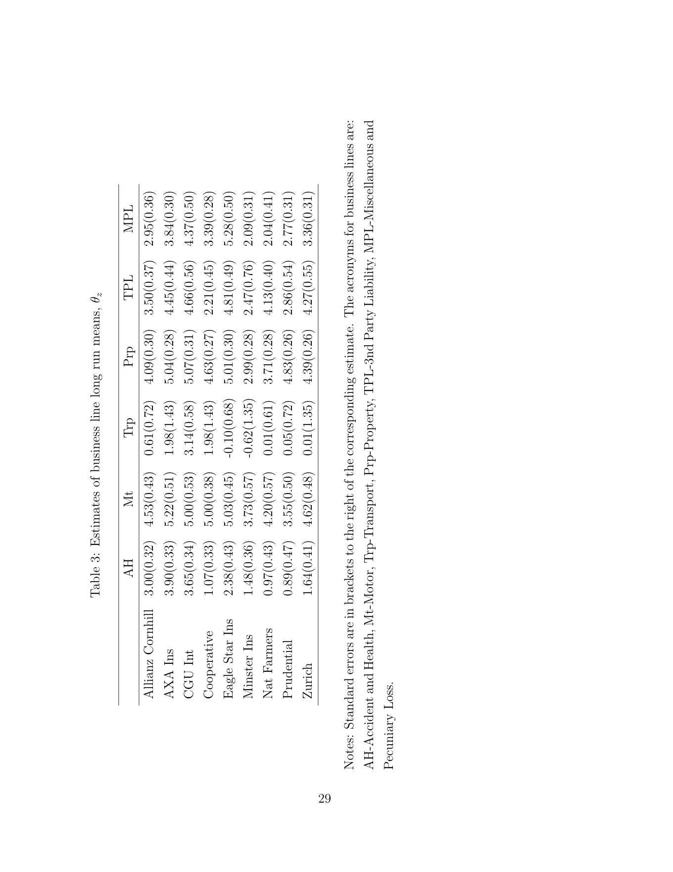
Using the net cash flow time series, we estimate a set of parameters θz, σz, αz by Maximum Likelihood estimation for each business line. In performing the estimations, we pool the data from the 9 different UK non-life insurers. For each business line, we estimate a single convergence parameter αz but allow the two other parameters θz and σz to vary across the different firms. Hence, for each business line we estimate (2×9)+1 parameters.

Standard errors are shown Parameter estimates for θz are presented in Table 3. in parentheses to the right of the estimates themselves. In most cases, the long term mean of a business line is reasonably stable across different firms. Among them, Motor insurance and Property insurance have higher mean level, whereas Accident and Health and Third Party Liability have lower mean. Across different insurance business lines, AXA tends to have higher mean, while Minister Insurance tends to have lower mean.

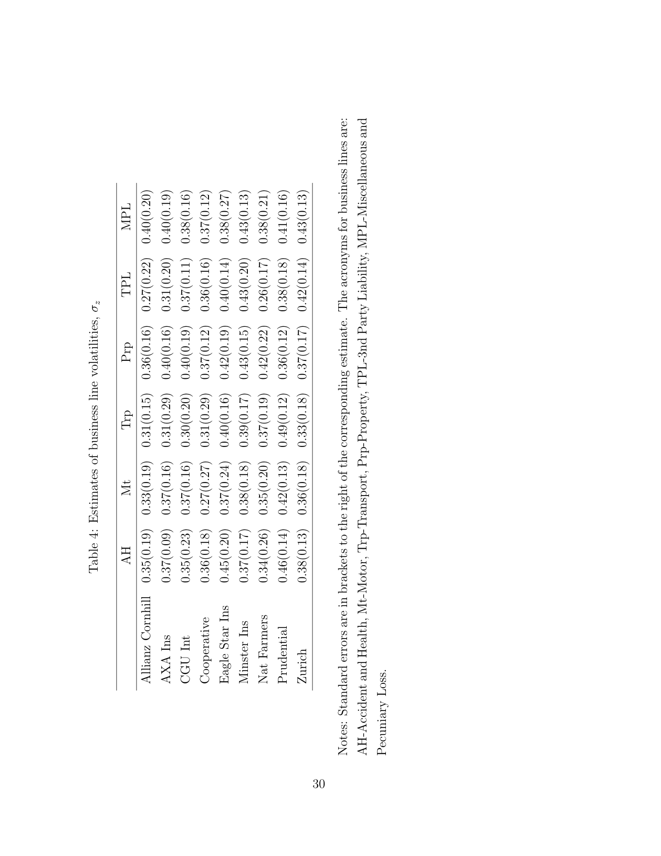
Table 4 presents parameters estimates for the volatilities, σz. The volatilities appear stable across different business lines and insurers, with range between 25%-45%. Estimates of mean reversion rates for each business line, αz, are presented in Table 5. Property and Miscellaneous and Pecuniary Loss tend to have low mean reversion, while Transport has high mean reversion rate. In all the tables containing estimates, standard errors are also presented in parentheses to the right of the estimate.

We perform similar estimations to obtain the interest rate parameters, θr, σr and αr. The interest rate data employed is one-year sterling Treasury bill rates observed annually over the same period 1985 to 2003. The parameter estimation for interest rate model is presented in Table 6. It shows that over the sample period the average of interest rate is around 3%, the mean reversion is slightly stronger than Motor insurance with 84%.

To be able to calculate the capitalised values of the business line cash flows, requires that one know not just the parameters described above but also the risk premiums, θz∗ − θz. A simple way to obtain these is to suppose that risk is priced in a way that is consistent with the Capital Asset Pricing Model (CAPM). In this case, we may suppose that:

θz∗ − θz = βz,M(θM − θr) (12)

Here, βz,M s the regression coefficient of the innovations εz,t+1 on an equity market index return rM,t+1 and θM = E (rM,t+1|Ft). We estimate βz,M and θM using annual returns data on the FTSE100 index and the zt+1 innovations obtained from the regressions described above.

4 Risk Calculations

Having estimated the parameters of the cash flow, interest rate and stock price processes, we construct time series of the fitted residuals, εbz,t+1 for each insurance business line, εbr,t+1 for interest rates and εbs,t+1 for the stock index and estimate their correlation matrix. Estimates of the correlations between the fitted innovations for insurance line, interest rate and stock index risks are reported in Table 7.

The correlations between different insurance lines are positive in most cases. This is to be expected given that the lines include premiums and costs which are likely to move together. Property and motor lines are particularly strongly positively correlated which is significant given that a large fraction of most companies’ total premium income (and hence presumably much of the risk) comes from these two lines.

It is perhaps surprising that interest rates changes exhibit a positive correlation with innovations in most of the insurance lines. One might expect that in recessions, interest rates will fall and claims on property and motor would rise (due to higher crime levels). However, UK interest rates in the recession of the early 1990s were high so one must interpret cyclical patterns and correlations with care.

The correlations between credit risk factor innovation εc,t+1 and the other innovations is harder to estimate as we do not have direct observations of a fitted version of the εc,t+1. Several authors have recently examined correlations between credit and market risk, focussing particularly on correlations between credit risk and interest rate changes. Estimates for relatively short horizons such as one month suggest that interest rate and credit spread changes have a marked negative correlation (see Duffee (1998)). However, correlations over longer periods appear to be close to zero (see Morris, Neal, and Rolph

(1999) and Kiesel, Perraudin, and Taylor (2001)). In what follows, we shall suppose that credit risk and innovations in other types of risk have a zero correlation.

The simulation exercises the results of which we report below consist of calculations of the economic capital needed by standalone banks and insurers and bancassurance groups comprising both banking and insurance operations. We chose to combine our insurance companies with a sizeable but not overwhelmingly large bank, to be specific one with loans worth 80 billion GBP. To put this in context, Barclays had loans worth approximately 155 billion GBP in 2003 while the medium sized bank Abbey National (subsequently taken over by Santander) had loans worth approximately 80 billion GBP.

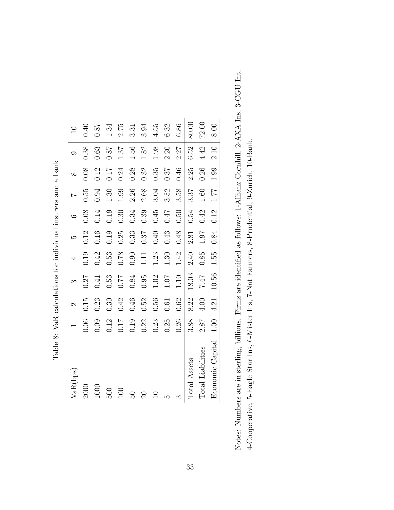
Table 8 reports the results of model simulations for standalone insurance companies and banks. The upper block of numbers in the table shows the absolute capital levels required to deliver a confidence level equal to a range of figures from 80% (see the 2000 basis point line) to 99.97% (see the 3 basis point line). The lower block of figures contains asset liability and economic capital numbers measured again in absolute terms in the form of billions of sterling. Columns 1 to 9 of the table show results for individual insurance companies while the right hand column gives results for the notional bank with loans of 80 billion described above.

The first point of interest is the confidence level that is delivered by the levels of economic capital shown in the last row of the table. For the larger, better-capitalised insurers (the insurers are sorted so that firms with higher total group premium income are to the left of the table), the confidence level implied by economic capital is extremely great. The probability of failure for the largest 3 insures is substantially less than 3 basis points. There are two firms for which the economic capital is small, namely Mister Ins and Nat Farmer for which the probability of failure is between 5 and 20% per annum.

Based on economic capital, the failure probability for the notional bank, with lending worth 80 billion, shown in Table 8 is less than 3 basis points. Based on regulatory capital equal to 8% of assets, the failure probability would also be less than 3 basis points. Under the 1988 Basel Accord, only half of the 8% capital must be held in the form of equity. One might argue that non-equity forms of capital will not prevent failure even if they limit losses to depositors if failure should occur. In this case, the regulatory capital relevant for deducing the confidence level would be 3.2 billion and the failure probability for our notional bank would be slightly less that 1%. Of course, many banks will hold not just the corporate loans assumed in our simulations but also large amounts of retail lending. Retail debt is generally thought to be lower risk than typical corporate loan portfolios so introducing retail debt into our example would imply a higher confidence level.

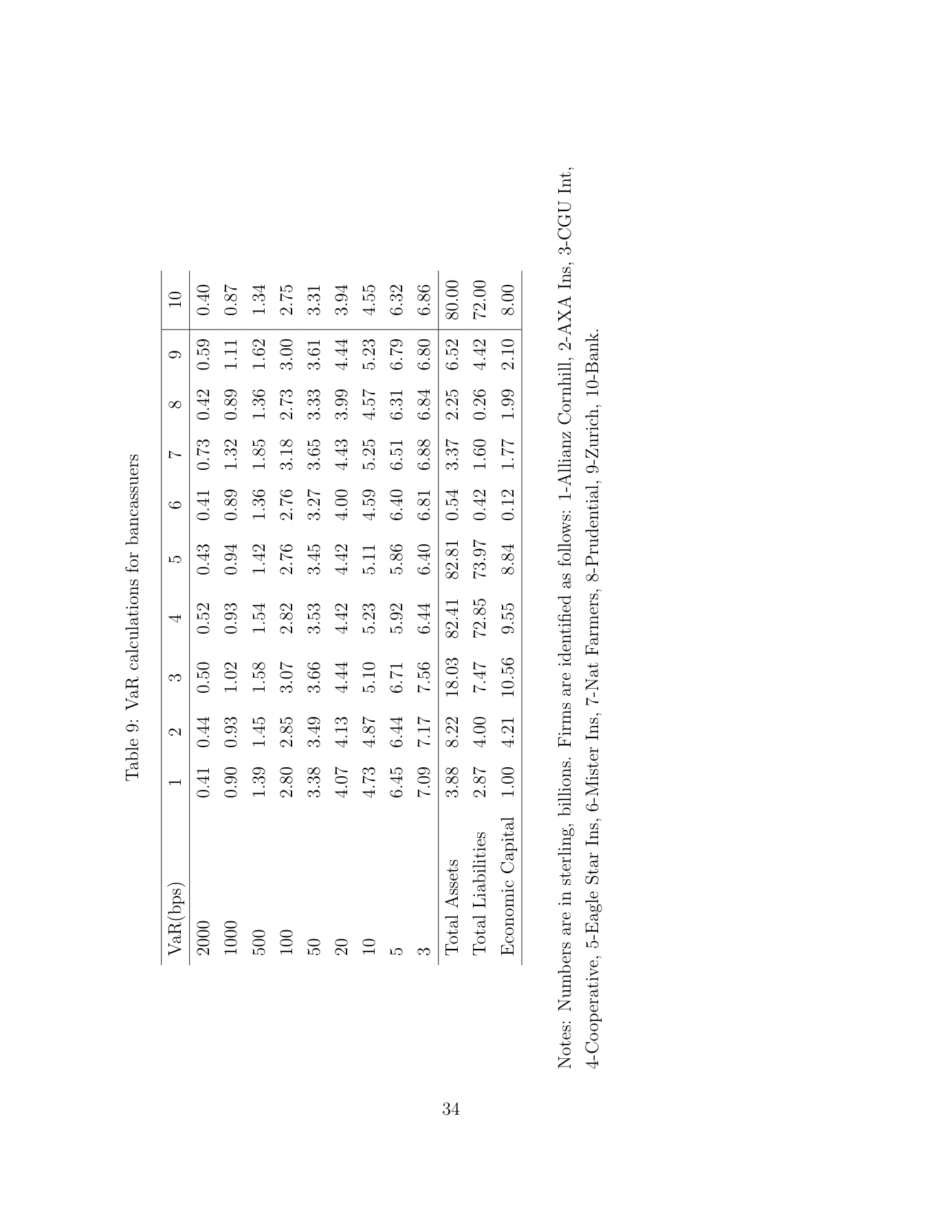
Now, suppose that the notional bank took over one of the insurers to form a bancassurers. Table 9 shows capital levels corresponding to different failure probabilities for bancassurers made up of our bank and insurers. Is risk increased or decreased by the merger? The result depends inevitably on how one assumes the bank finances the acquisition. If it finances the acquisition by issuing more deposit, the capital of the bancassurer will equal that of the bank prior to the transaction so obviously the confidence level for the bank will decline. However, the results in Table 8 suggest that if financing includes even a small additional amount of equity, the risk of the bancassurers will be lower than the standalone bank since the amounts of capital necessary to maintain given confidence levels are only slightly larger than those needed to maintain the same confidence levels for the bank alone.

Table 9 shows economic capital figures for various failure probabilities summed across the notional bank and the individual insurers. Effectively, these show the combined level of capital that would be needed in the bank and the insurer if both are to have a failure rate equal to some specified level. Comparing these figures with those in Table 8, it is clear than the diversification benefits of forming the bancassurer are considerable.

5 Conclusions

This study has devised and implemented for a sample of UK non-life assurers a risk management model that allows one to calculate the failure probabilities of the firms in question alone or in combination with a bank. The model generalises the ratings based credit risk model widely employed by firms and regulators to assess banking book credit risk and to parameterise capital requirements for the new Basel Accord. Extending this model to include insurance lines permits one to assess the failure probabilities implicit in current levels of insurer economic and regulatory capital and to examine the implications for risk of mergers between banks and insurers.

Our analysis shows that mergers may have sound economic justification through the economies they permit in economic capital. Bank and insurer combinations can achieve the same confidence level with much less capital than the institutions are currently holding collectively. There may, of course, be other economic motives for mergers such as economies of scale in the distribution of retail financial products (see, for example Mhlnickel and Wei (2015)) but these are beyond the scope of this research. We also show that the default probabilities implicit in prevalent levels of non-life insurer economic capital are very low except for two cases where the firms involved were subsidiaries of larger entities.

Appendix

A1 Derivation of Exponential Vasicek Model

This section shows the mathematical details of how to model insurance business line in the framework of exponential Vasicek Model.

A1.1 Assumptions and notations

Suppose rt is the continuously compounded annual interest rate from year t to t − 1, and it follows an AR(1) process

rt+1 = θr + αr(rt − θr) + εr,t+1

where εr,t are i.i.d. N(0, σr[2]) and is independent from rt. Denote ezt+1 − k

the loss of an insurance business line from year t to t+1 realised at t+1. Where zt is another AR(1) zt+1 = θz + αz(zt − θz) + εz,t+1 N(0, σ[2] Although εz,t are i.i.d. z) and is independent from rz, it contemporaneously correlates to εr, such that E(εr,tεz,t) = ρrzσrσz

We need to use above setup to calculate

• a zero coupon bond, P (t + n) where n is time to maturity.

• accrued insurance loss V (t, t + n).

A1.2 Valuation of zero coupon bond

To calculate the value of a zero coupon bond, we used standard formula

n " ! # X P (t, t + n) = E exp − ri |Ft i=1

Note this expectation is taken under risk neutral measure, to easy notation we assume that the two AR(1) processes given previously are in the risk neutral world. Since the sum of AR processes are still normal, taking exponential function on it becomes lognormal. To calculate the expectation of log-normal random variable we just need to figure out its conditional mean and variance.

By recursive substitution rt+i can be written as rt+i − θr = αri (rt − θt) + αri−[1]εr,t+1 + · · · + εr,t+i

So E [rt+i|Ft] = θr + αri (rt − θt) Sum over all i end up with " n # 1 − αrn X E rt+i|Ft = nθr + (rt − θr)αr 1 − αr i=1

i=1 ri, expand ri inside the Next we need to calculate the conditional variance of Pn summation n n X rt+i = X αri−1εr,t+1 + αri−2εr,t+2 + · · · + εr,t+i i=1 i=1 In the above the coefficient of εt+1 is 1, α, α[2], · · · , αn−[1].

The coefficient of εt+2 is 1, α, α[2], · · · , αn−[2].

And so on so forth.

Therefore the value of zero coupon bond is

n ! X Var rt+i|Ft i=1 1 − αrn 1 − αrn−[1] = Var εr,t+1 + εr,t+2 + · · · + εr,t+n 1 − αr 1 − αr σr [2] = (1 − αrn)[2] + (1 − αrn−[1])[2] + · · · + (1 − αr)[2] 1 − αr σr [2] 1 − αrn 1 − αr[2]n = n − 2αr + αr[2] 1 − α[2] 1 − αr 1 − αr r

Finally the zero coupon bond price can be written as

1 − αrn P (t, t + n) = exp − nθr + (rt − θr)αr 1 − αr 1 σr [2] 1 − αrn 1 − αr[2]n ) + n − 2αr + αr[2] 2 1 − αr 1 − αr 1 − αr[2]

A1.3 Valuations of Insurance business line

The value of an insurance business line, like zero coupon bond, is the expected present value of future cash flow under risk neutral world. Denote V (t, t + n) the value of a business line and the cash flow is looking forward for n years. So

i " n ! # X X V (t, t + n) = E (exp (zt+i) − k) exp − rt+j |Ft i=1 j=1 i n " n ! # X X X = E exp zt+i − rt+j |Ft − k P (t, t + i) i=1 j=1 i=1

The 2nd term is known from previous section, the 1st term, again, is log-normal. So to calculate the expectation in the 1st term we need to figure out the conditional mean and variance of i X rt+j zt+i − j=1

Using the property of Zt which is AR(1) process

= E (zt+i|Ft) θz + αzi (zt − θz) 1 − αz[2]i = σ[2] Var (zt+i|Ft) ε 1 − αz[2]

The conditional mean is

i ! 1 − αri X E zt+i − rt+j|Ft = θz + αzi (zt − θz) − iθr + (rt − θr)αr 1 − αr j=1

The conditional variance is

i ! X Var zt+i − rt+j|Ft j=1 i i ! ! X X = Var (zt+i|Ft) + Var rt+j|Ft − 2Cov zt+i, rt+j|Ft j=1 j=1

Only the 3rd term is unknown, which can be calculated by the following:

i " # X Cov zt+i, rt+j|Ft j=1 = Cov αzi−[1]εz,t+1 + αzi−[2]εz,t+2 + · · · + εz,t+i, 1 − αri 1 − αri−[1] + εr,t+1 εr,t+2 + · · · + εr,t+i 1 − αr 1 − αr αz = σzσrρzr αzi (1 − αri ) + αzi−[1](1 − αri−[1]) + · · · + αz(1 − αr) 1 − αr 1 − αi σzσrρzrαz[2] z 1 − (αrαz)i = − αr 1 − αr 1 − αz 1 − αrαz

Finally the present value of the insurance business line is

V (t, t + n) n 1 − αri X = exp θz + αzi (zt − θz) − iθr − (rt − θr)αr 1 − αr i=1 σz[2] 1 − αz[2]i σr[2] 1 − αri 1 − αr[2]i + + i − 2αr + αr[2] 2 1 − αz[2] 2(1 − αr)[2] 1 − αr 1 − αr[2] σzσrρzrαz[2] 1 − αzi 1 − (αrαz)i − − αr − k P (t, t + i) 1 − αr 1 − αz 1 − αrαz

References

Allen, L., and J. Jagtiani (2000): “The Risk Effects Of Combining Banking, Securities, And Insurance Activities,” Journal of Economics and Business, 52(6), 485–497.

Amel, D., C. Barnes, F. Panetta, and C. Salleo (2004): “Consolidation And Efficiency In The Financial Sector: A Review Of The International Evidence,” Journal of Banking and Finance, 28(10), 2493–2519.

Babbel, D., and C. Merrill (1997): “Economic valuation models for insurers,” Center for financial institutions working papers, Wharton School Center for Financial Institutions, University of Pennsylvania.

Boyd, J., S. Graham, and R. Hewitt (1993): “Bank holding company mergers with nonbank financial firms: Effects on the risk of failure,” Journal of Banking and Finance, 17(1), 43–63.

Carow, K. (2001): “Citicorp-Travelers Group Merger: Chanllenging Barriers Between Bankin Gand Insurance,” Journal of Banking and Finance, 25, 1553–1571.

Chen, Z., D. Li, L. Liao, F. Moshirian, and C. Szablocs (2009): “Expansion And Consolidation Of Bancassurance In The 21st Century,” Journal of International Financial Markets, Institutions and Money, 19(4), 633–644.

Chen, Z., and J. Tan (2011): “Does Bancassurance Add Value For Banks? - Evidence From Mergers And Acquisitions Between European Banks And Insurance Companies,” Research in International Business and Finance, 25(1), 104–112.

Cummins, J. D., and R. D. Phillips (1999): “Applications of Financial Pricing Models In Property-liability Insurance,” Discussion paper, The Handbook of Insurance Economics.

De Jonghe, O. (2010): “Back To The Basics In Banking? A Micro-Analysis Of Banking System Stability,” Journal of Financial Intermediation, 19(3), 387–417.

Dixit, K., and S. Pindyck (1994): Investment Under Uncertainty. Princeton University Press:Princeton, New Jersey.

Dreassi, A., and M. C. Schneider (2015): “Bancassurance and Scale Economies: Evidence from Italy,” The Geneva Papers on Risk and Insurance, 40(1), 89–107.

Duffee, G. R. (1998): “The Relationship Between Treasury Yields and Corporate Bond Yield Spreads,” Journal of Finance, LIII(6), 2225–2241.

England, P., and R. Verrall (2002): “Stochastic Claims Reserving In General Insurance,” Discussion paper, Institue of Actuaires.

Filipovi´c, D., and M. Kupper (2008): “Optimal Capital And Risk Transfers For Group Diversification,” Mathematical Finance, 18(1), 55–76.

Gordy, M. (2000a): “A Comparative Anatomy of Credit Risk Models,” Journal of Banking and Finance, 24(1-2), 119–149.

(2000b): “Credit VaR and risk-bucket capital rules: a reconciliation,” Proceedings of the 36th Annual Conference on Bank Structure and Competitions, pp. 406–417.

Hoyt, B. E., and J. S. Trieschmann (1991): “Risk/Return Relationships for Life- Health, Property-Liability, and Diversified Insurers,” The Journal of Risk and Insurance, 58(2), 322–330.

IAIS (2009): “Issues Paper on Group-Wide Solvency Assessment and Supervision,” Discussion paper, International Association of Insurance Supervisions.

Keller, P. (2007): “Group Diversification,” The Geneva Papers on Risk and Insurance

- Issues and Practice, 32(3), 382–392.

Kiesel, R., W. R. Perraudin, and A. P. Taylor (2001): “The Structure of Credit Risk,” Working Paper 131, Bank of England.

Laeven, L., and R. Levine (2007): “Is There A Diversification Discount In Financial Conglomerates?,” Journal of Financial Economics, 85(2), 331–367.

Luder, T. (2007): “Modelling of Risks in Insurance Groups for the Swiss Solvency Test,” Bulletin of the Swiss Association of Actuaries, 1, 81–97.

Mack, T. (1993): “Distribution-free Calculation Of The Standard Error Of Chain- Ladder Reserve Estimates,” ASTIN Bulletin, 23, 214–225.

M¨alk¨onen, V. (2004): “Capital Adequacy Regulation And Financial Conglomerates,” Research Discussion Papers 10/2004, Bank of Finland.

Mhlnickel, J., and G. N. F. Wei (2015): “Consolidation and systemic risk in the international insurance industry,” Journal of Financial Stability, 18, 187–202.

Morris, C., R. Neal, and D. Rolph (1999): “Credit spreads and interest rates,” Working paper, Indiana University.

Morrison, A. (2003): “The Economics Of Capital Regulation In Financial Conglomerates,” Geneva Papers On Risk And Insurance-Issues And Pratics, 28(3), 521–533.

Nakada, P., H. Shah, U. Koyluoglu, and O. Collignon (1999): “P&C RAROC: A catalyst for improved capital management in the property and casualty insurance industry,” Journal of Risk Finance, pp. 1–18.

Nickell, P., W. R. Perraudin, and S. Varotto (2000): “The Stability of Ratings Transitions,” Journal of Banking and Finance, 24(1-2), 203–227.

Ohlsson, E., and J. Lauzeningks (2009): “The One-Year Non-Life Insurance Risk,” Insurance: Mathematics and Economics, 45, 203–208.

Schmeiser, H., and C. Siegel (2010): “Regulating Insurance Groups: A Comparison Of Risk-Based Solvency Models Hato Schmeiser,” Working Paper on Risk Management and Insurance 79, University of St. Gallen.

Slijkerman, J. F., D. Schoenmaker, and C. G. de Vries (2013): “Systemic risk and diversification across european banks and insurers,” Journal of Banking Finance, 37(3), 773–785.

van Lelyveld, I., and A. Schilder (2003): “Risk in Financial Conglomerates: Management and Supervision,” Research Series Supervision 49, De Nederlandsche Bank.

Vasicek, O. A. (1977): “An Equilibrium Characteristic of the Term Structure,” Journal of Financial Economics, 5, 177–188.

Wilkie, A. D. (1995): “More on the stochastic asset model for actuarial use,” British Actuarial Journal, 1(5), 777–964.

Winter, R. A. (1991): “The liability insurance market,” Journal of Economic Perspectives, 5, 115–136.

(1994): “The dynamics of competitive insurance markets,” Journal of Financial Intermediation, 3, 379–415.

Tables and Figures

Table 1: Premium income by insurance line (as % of total premium)

AH Mt Trp Prp TPL MPL Allianz Cornhill 2.01 37.77 0.09 29.54 9.10 21.43 AXA Ins 36.53 20.43 0.97 26.01 13.07 2.24 CGU Int 2.43 5.78 0.95 24.44 9.79 4.98 Cooperative 0.31 70.23 0.00 26.92 1.72 0.06 Eagle Star Ins 10.54 30.21 0.00 23.87 8.23 9.43 Minster Ins 0.14 0.00 0.00 11.38 21.20 67.55 Nat Farmers 1.83 53.06 0.37 28.26 12.49 3.07 Prudential 49.66 6.80 1.02 16.15 24.05 2.33 Zurich 0.73 38.40 0.05 33.36 23.72 2.45

Notes: The acronym for business lines are: AH-Accident and Health, Mt-Motor, Trp-Transport, Prp-Property, TPL-3nd Party Liability, MPL-Miscellaneous and Pecuniary Loss.

Table 2: Asset values as a percentage of total assets for each insurer

Gbond Stock Cbond LnMg Cash ReIns Allianz Cornhill 29.73 8.79 4.11 35.71 1.50 22.37 AXA Ins 20.89 14.57 13.14 29.78 0.39 3.11 CGU Int 15.57 11.84 0.75 33.84 0.49 10.43 Cooperative 35.42 29.60 20.67 16.70 0.12 0.87 Eagle Star Ins 12.64 10.11 0.21 33.28 3.77 24.26 Minster Ins 36.24 3.33 4.65 11.01 2.24 46.29 Nat Farmers 20.69 47.28 8.72 28.91 0.13 1.43 Prudential 5.54 18.10 0.00 14.33 8.69 5.68 Zurich 28.93 7.86 23.39 31.53 0.95 8.69

Notes: The acronyms for business lines are: AH-Accident and Health, Mt-Motor, Trp-Transport, Prp-Property, TPL-3nd Party Liability, MPL-Miscellaneous and Pecuniary Loss.

Table 5: Estimates of business line mean reversions, αz

Alpha Se Accident and Health 0.56 0.22 Motor 0.67 0.21 Transport 0.76 0.21 Property 0.44 0.23 Third Party Liability 0.66 0.22 Misc. and Pecuniary Loss 0.45 0.20

The convergence parameters are assumed to vary only for different business line but not across firms.

Table 6: Estimates of interest rate parameters

Estimates Se α 0.84 0.17 σ 1.11 0.24 θ 3.03 2.74

The interest rate data employed is one-year sterling Treasury bill rates observed annually over the same period 1985 to 2003.

Table 7: Correlation estimation for ϵij

AH Mt Trp Prp TPL MPL Int Stock AH 100 8 -13 27 1 9 -3 1 Mt 8 100 3 37 22 -11 17 29 Trp -13 3 100 11 -0 -6 20 10 Prp 27 37 11 100 35 15 -4 -6 TPL 1 22 -0 35 100 32 -7 -14 MPL 9 -11 -6 15 32 100 -8 -7 Int -3 17 20 -4 -7 -8 100 31 Stock 1 29 10 -6 -14 -7 31 100

Notes: The acronyms for business lines are: AH-Accident and Health, Mt-Motor, Trp-Transport, Prp-Property, TPL-3nd Party Liability, MPL-Miscellaneous and Pecuniary Loss.

Table 3Copy link

Table 4Copy link

Table 8Copy link

Table 9Copy link

Notes

∗The authors may be contacted at william-perraudin@riskcontrollimited.com and siy- izhou@hotmail.com. 1Reserve and premium risks relates to past and future claims respectively.