This paper formulates a simulation model of a bank balance sheet and analyzes optimal choices of portfolio credit quality and funding maturity under different assumptions about liquid assets requirements that may be imposed by regulators. We employ industry standard approaches to modelling portfolio payoffs. Funding costs are assumed to rise if impairment in asset quality generates a decline in the bank’s rating. We parameterise the model to be consistent with balance sheet data for two large UK banks at end 2009.
Executive Summary
This paper formulates a simulation model of a bank balance sheet and analyzes optimal choices of portfolio credit quality and funding maturity under different assumptions about liquid assets requirements that may be imposed by regulators. We employ industry standard approaches to modelling portfolio payoffs. Funding costs are assumed to rise if impairment in asset quality generates a decline in the bank’s rating. We parameterise the model to be consistent with balance sheet data for two large UK banks at end 2009.
We examine the impacts on bank asset-liability choices of the two liquidity standards proposed by BCBS (2009): (i) a requirement that banks hold sufficient liquid assets to survive a funding stress scenario designed by regulators and (ii) a requirement that bank liabilities weighted according to their relative stability exceed assets weighted according to their relative illiquidity. (ii) represents a potential constraint on bank asset-liability choices whereas (i) consists of a bank specific requirement to hold liquid assets at no lower than a given level.
According to our calculations, the constraint in (ii) does not bind for the two banks we examine. We model (i) as an exogenous upward shift from current levels in liquid asset holdings. Both banks we examine held liquid assets at around 7% at end 2009.
We experiment by raising the liquid asset requirement in (i) to 10% and 12.5% of assets. For both banks, the effect is to increase the short-term funding and bank employs and to induce it to hold more risky assets.
1. Introduction
The crisis of 2007-2008 involved a major collapse in the availability of bank liquidity. Losses on opaque structured products generated concerns about the solvency of many banks, disrupting interbank lending. Over-night interbank markets became the only way in which banks could obtain funding (except though central bank intermediation) and interbank spreads at longer maturities soared. (Brunnermeier
(2009) and Taylor and Williams (2008) provide descriptions of the crisis.)
The crisis brought into question the capital-focused approach to banking regulation that has held sway since the early 1980s. At that time, a consensus emerged (embodied in the 1988 Basel Accord) that the primary tool of banking regulation should be capital. While the recently enacted Basel II rules contained a general requirement that banks manage their liquidity risk, this requirement represented a minor and relatively non-binding part of the package of measures.
Now, banks and their regulators have woken up to the fact that being solvent is not enough. A bank must also ensure that its funding is stable. Otherwise it may be subject to crises of confidence or runs affecting its wholesale funding and possibly, even its retail deposits if deposit insurance coverage is incomplete. The potential for such runs has been extensively studied (see for example Diamond and Dybvig (1974)) but regulators and firms had lost sight of its empirical relevance for large, well-diversified banking institutions.
The regulatory response to the newly perceived importance of funding risk has been to propose liquidity standards for banks. BCBS (2009) contains proposals on liquidity standards for internationally active banks. A year earlier, the UK’s Financial Services Authority (FSA) had issued rules and guidance on liquidity monitoring and management for a wide set of UK financial firms including insurers and securities firms as well as banks (see FSA (2008)).
The Basel document (BCBS (2009)) proposes placing two important new requirements on internationally active banks. First, banks will be obliged to hold liquid assets sufficient to withstand the significant curtailment of available funding for a onemonth period. The scenario that the bank’s funding approach must be able to withstand will be provided by the bank’s supervisor in the form of a bank-specific stress test. This requirement is called the Liquidity Coverage Ratio (LCR).
What exactly constitutes liquid assets in this context has been contentious. The most conservative option would be to define liquid assets as Treasury bills and central bank deposits. More broadly, it might include high quality sovereign bonds. Broader still would be to include high quality corporate bonds and even possibly some of the assets that central banks have recently accepted as repo collateral, namely structured products.
The second liquidity requirement proposed by BCBS (2009) obliges banks to maintain adequate levels of stable funding relative to the marketability of its assets. The restriction is expressed in the form of a requirement that available stable funds (calculated as a weighted average of different funding types with weights reflecting the stability and reliability of the funding source) must exceed a weighted average of assets (where the weights this time reflect the degree to which assets would prove difficult to liquidate in a crisis). This requirement is called the Net Stable Funding Ratio (NSFR).
The NSFR may be viewed as a linear restriction on possible combinations of assets and liabilities that the bank is permitted to hold. If it binds, this restriction will constrain what combinations of assets and liabilities banks may hold.
Instead, the LCR is simply a requirement placed on banks by regulators to hold adequate liquid assets. Conceivably this might also be thought of as a restriction on acceptable asset-liability combinations but since it is less clearly parametric in approach, we will treat it in our analysis as a requirement to boost liquid assets.
Banks may satisfy the new requirements by altering their asset allocation, substituting liquid assets for the less liquid assets in their portfolios. Alternatively, they may satisfy the ratios by altering the balance of their funding between short- and long-dated funding instruments.
Natural and important questions to ask are: how and to what extent banks’ behavior may be affected by the new liquidity standards and how much will this affect the wider macro-economy? These questions are the subject of this paper.
Specifically, this paper analyzes the likely impact of liquidity regulations on banks asset and liability maturity choices using a microeconomic model of banks’ balance sheets. We formulate a stochastic simulation model of a bank’s equity and parameterize this for several large UK banks.
We then proceed by simulating the pay-off on the equity interest in the balance sheet for different choices of asset quality and funding maturity profile. We determine the optimal portfolio and funding choices of banks under different assumptions about risk aversion.
The analysis is performed, as far as possible, using industry standard techniques for modeling loan losses, credit quality and term structures. To this extent, the calculations may be thought of those that would be performed by a quantitative analyst working in a bank tasked with analyzing how the bank’s asset-liability decisions should be altered in the light of new liquidity regulations.
The stochastic behavior of the bank’s credit portfolios (either loans held in the banking book or negotiable credit instruments held in the trading book) is modeled using diversified pool exposures (which generalize the well-known Vasicek loan loss distribution) developed by Lamb and Perraudin (2008).
We model the choice of funding maturity within a stochastic model of the term structure. The bank is influenced by the need to balance the duration of assets and liabilities given the relative cost of short and long funding. We also build into the model, however, the fact that the bank is influenced by possible increases in its funding costs if its own rating declines.
Our calculation is stylized and we do not have full information about banks’ balance sheets. It is nevertheless interesting to note that, for the two banks we examine, the linear constraint on assets and liabilities fails to bind with the current configurations of assets and liabilities that we observe in our two banks. This may reflect the fact that banks currently (so soon after a major banking crisis) possess relatively defensive balance sheets. This might no longer be true at some point in the future when funding has become easier and the discount on illiquid assets is not so great.
However, when we introduce a requirement (based, say on a supervisor-imposed stress scenario) that liquid assets rise from their current level of 7% to 10% and then 12.5%, we observe significant substitution effects, with our two banks both increasing their short-term financing and the riskiness of their assets.
Our analysis of liquidity requirements is comparable to past studies of how capital requirements affect bank portfolio choice. Kim and Santomero (1998) employ a simple mean-variance framework to argue that increases in the level of non-risksensitive capital requirements could induce banks to substitute significantly towards higher risk assets. Blum (1998) finds comparable results in a dynamic model. Calem and Rob (1999) employ dynamic models to examine risk-sensitive capital requirements and suggest that higher capital may at first lower and then increase risk taking.
The structure of this report is as follows. Section 2 describes the relevant literature on liquidity. Section 3 discusses empirical and theoretical evidence on how banks may react to liquidity standards. Section 4 sets out our microeconomic simulation model. Section 5 presents the results when the model is a parameterized to match features of two large UK banks. Section 6 concludes.
2. Literature
A substantial literature on liquidity has emerged in recent years. This includes
(i) Studies of the impact on the prices of traded securities of their (market) liquidity,
(ii) Studies of how levered financial firms and in particular banks are affected by
(funding) illiquidity in their balance sheets,
(iii) Recent papers that have attempted to study how funding and market liquidity interact in equilibrium.
In this section, we summarize the main contributions to this literature and then draw conclusions relevant for liquidity regulation in banks.
The impact of liquidity on the prices of assets or alternatively the expected returns on assets has been examined by many studies. Significant contributions include Amihud and Mendelson (1986), Silber (1991), and Pastor and Stambaugh (2001) on equity securities, and Amihud and Mendelson(1991), Warga (1992), Kamara (1994), Elton and Green (1998), and Krishnamurthy (2001) on Treasury bond. Delianedis and Geske (2002), Houweling, Mentink and Vorst (2005), Longstaff, Mithal and Neis (2005), De Jong and Driessen (2006), Chen, Lesmond and Wei (2007) and Perraudin and Taylor (2007) study the effects of liquidity on corporate bond spreads.
Primarily empirical, the studies in this literature either examine the association between proxies for illiquidity and discounts or additional expected returns in securities or attempt to identify pricing differences between exposures to the same risk attributable to liquidity differences.
Several theoretical papers (see Allen and Gale (1994), Dow (2004) and Plantin (2008)) have examined what influences liquidity in individual instruments in particular focusing on how liquidity may be self fulfilling and there may alternative equilibriums with high and low liquidity.
In the model we develop below, shocks to asset values are driven by credit factors rather than a combination of credit and liquidity factors. The parameterization of portfolio value change volatility is however conservative so one could think of the return volatility that arises as including both types of volatility even if the modeling of liquidity is not explicit.
The literature on funding liquidity is closely linked to the strand of banking theory that emphasizes bank maturity transformation and the cost of liquidating bank loan books early. Classic contributions by Bryant (1980) and Diamond and Dybvig (1983) suggest that the sequential nature of bank deposit withdrawals together with the illiquid nature of bank assets creates the possibility of multiple equilibriums some of which involve banks runs and some of which do not.
More recently, Diamond and Rajan (2005) have argued that bank runs help to mitigate agency problems between banks and their outside investors. Specifically, they argue that the possibility of runs allows banks to commit to exercising their relationship banking expertise and hence makes the equilibrium more efficient. In the presence of stochastic shocks, banks hold capital to prevent value-reducing runs so the determination of capital and optimal allocations between liquid and illiquid assets and liabilities are tightly connected.
Following the recent crisis, a new literature on liquidity and financial market frictions has emerged including amongst others Acharya and Viswanathan (2008), Acharya, Yorulmazer and Shin (2007), Adrian and Shin (2008), Shin (2006) and Brunnermeier and Pedersen (2008). These papers stress moral hazard problems as market friction.
A smaller set of papers (see Gorton and Pennacchi (1990) and Parlour and Plantin (2008)) have touched on the issue of asymmetric information’s effect on liquidity.
While these papers provide insightful analysis of how illiquidity crises may arise and may feed back into funding problems for financial firms, they do not shed light directly on how liquidity considerations affect the more detailed asset-allocation of banks. Given that formal regulation of liquidity has not been a feature of the Basel approach until very recently, it is not surprising that no papers have examined how the imposition of liquidity requirements on banks could affect their behavior.
3. Modelling a bank balance sheet and equity payoffs
a. Summary of model components
To examine the impact on bank choices of liquidity requirements, we formulate a stochastic model of a bank balance sheet. The asset side of the balance includes loans of different credit qualities. Liabilities include deposits of different maturities. Liquidity risk is included by supposing that the spreads on funding depend on the bank’s own rating which fluctuates as losses on the asset side of the balance sheet are experienced.
Since we wish to analyze the optimal asset-liability decisions of banks, we simulate the banks’ balance sheets with different portfolios, parameterized using UK bank data, and examine how their optimal choices of assets and liabilities are affected by requirements that they hold liquid asset buffers and/or satisfy restrictions on the maturity structure of their funding.
We focus on two large UK banks, namely Lloyds-TSB and Barclays. In each case, we model the banking book as consisting of differently rated credit exposures and the trading book as split between (i) cash (i.e., Treasury bills and central bank deposits),
(ii) a credit portfolio and (iii) a log-normal payoff representing other trading book assets.
Assets
The building blocks for our modeling of credit portfolios are diversified pool exposures. These are constructed using a dynamic version of the Vasicek distributions of loan loss-rate. This distribution has been widely employed in the valuation and risk analysis of synthetic CDOs and serves as the basis for the capital charge formulae included in Basel II.
To understand the nature of these diversified pool exposures, consider an individual obligor denoted, i, that defaults at time t if a latent random variable Zi,t < -c for some constant c.
Suppose the Zi,t for t = 0,1,2… and i = 1,2,3…n satisfy a factor structure in that:
Zi,t = ρXt + 1− ρεi,t
Assume that:
X t = βX t−[1] + 1− βηt .
Here, εi,t and ηt are standard normal and independent for pairs of obligors i and j and across time t.
Note that the Xt has been constructed so that it has a unit unconditional variance. If Xt has unconditional unit variance then so to does Zi,t. The unconditional probability of default then satisfies:
Φ−[1](− c) = q .
Lamb and Perraudin (2008) show that, as the number of exposures becomes infinitely large, if θt is the fraction of the portfolio that has defaulted by date t and:
~ −1 , θ≡ Φ (θ)
The Law of Large Number then implies that:
1− β ρ 1− β ~ ~ −[1] . θt = βθt−[1] + Φ (q)− ηt 1− ρ 1− ρ
In other words, the transformed loss rate at t has a normal distribution:
⎛ 1 ⎞ ~ −[1] ~ − β −[1] ρ(1− β) θt ≡ Φ (θt ) → N βθt−[1] + Φ (q), ⎜⎝ 1− ρ 1− ρ ⎟⎠
Now, consider how the cash flows on a diversified pool exposure evolve over time. Suppose there is a specific contractual cash flow amount Ct paid by exposure type each period. The cash flow in the first period is:
cashflow[1] = C[1](1−θ[1])(1−θ[0] )
As losses are cumulative, the cash-flow in the second period is:
cashflow[2] = C[2] (1−θ[2] )(1−θ[1])(1−θ[0] )
Therefore, cash-flow in period t may be written as:
t cashflowt = Ct ∏(1−θi ) i=0
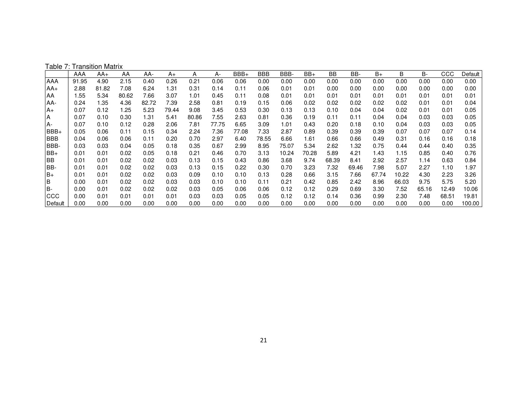
Given a set of cash-flows, Ct, parameters q, β and ρ, and an initial loss rate level, θ[0], one may simulate the behaviour of a diversified pool exposure. In fact, we assume a vector of q parameters corresponding to unconditional default cut-off points for each future year stretching forward. These are chosen to be consistent with the cumulative default probabilities implied by a standard ratings-transition matrix calculated using Moody’s historical data on ratings histories.
Liabilities
Interest rates are assumed to be stochastic and to be driven by a Libor market model of the term structure of interest rates. The Libor market model (see Brace, Gatarek and Musiela (1997)) is a variant of the forward interest rate term structure model of Heath, Jarrow and Morton (1992) but unlike the classic Heath-Jarrow-Morton model it places assumptions on discrete-time forward rates, supposing that they possess diffusion terms. This effectively means that forward interest rates are log-normal and hence always positive. The Libor market term structure model we employ is parameterized using historical data on pure discount bond prices extracted from UK gilts values.
We suppose that the banks’ liabilities are split between long-term funding with the same three-year maturity as the credit portfolios and short-term one-year funding. While this is a simplifying assumption, it allows us to capture the notion of maturity mismatch and refinancing or roll-over costs.
Recall that the bank’s credit portfolio, split between different ratings grades, has a three-year maturity. Banks may wish to issue short funding depending on the relative interest rate costs of doing so but they will be discouraged from funding by considerations (a) of asset-liability duration mismatch and (b) of the risks that if the bank’s rating declines, its cost of funds will increase.
This latter effect is clearly an important phenomenon to consider in any study of liquidity and bank balance sheet choices. We build such effects into our model by suppose that spreads adjust depending on the evolution of the bank’s rating. We model the rating using an ordered probit model of ratings evolution in which the risk factors are identical to those that drive the credit exposures of the bank (see Bhatia, Finger and Gupton (1997) for an exposition). If the rating is downgraded, the spread that the bank must pay on its short term borrowing rises sharply. The need to avoid this provides the bank with an additional motive to limit its dependence on short funding.
Model simulation
We simulate the model using one-year time steps and suppose that the banks’ decisions are made over a three-year horizon. The decisions are made based on a Hyperbolic Absolute Risk Aversion (HARA) utility function. HARA preference takes the form: 1 −ρ Utility = Et (U(WT )) where U(W ) ≡ (A + W )[1] 1− ρ We denote the power coefficient as ρ. As wealth increases, the intercept parameter A becomes less important and the coefficient of relative risk aversion approaches ρ. It is necessary to use the more general HARA class of preferences instead of Constant Relative Risk Aversion (i.e., the case when A=0) because equity pays zero with positive probability but U(W) goes to negative infinity as W approaches zero.
We reduce the dimensionality of the bank’s choices by supposing that the bank considers shifts in the credit quality of its credit portfolios by shifting portfolio shares in a proportional manner between (i) investment grade and (ii) sub-investment grade. For each bank, we employ data from regulatory returns on the breakdown of the bank’s IRB-business exposures between different default probability ranges.
For each bank, we map these default probability “buckets” to a set of seven discrete
(coarse) ratings categories, namely AAA, AA, A, BBB, BB, B and CCC. We then simulate the model under a set of different assumptions about the relative weightings of the investment grade and sub-investment grade portfolios, keeping the relative shares within each of these two sub-categories equal to the relative shares observed in the bank’s actual portfolio.
We again reduce the dimensionality of the bank’s funding decision by supposing that it splits its liabilities into one-year funding and funding with maturity equal to the maturity of the credit portfolio (namely three years). The one-year funding is rolled over each year up to the three-year horizon of the simulation and with the spread adjusting at each roll-over depending on the evolution of the bank’s rating (the modeling of which was described in the liability section above).
We simulate the bank’s balance sheet one million times and then evaluate the random payoff to equity-holders using von Neumann-Morgenstern preferences with a Hyperbolic Absolute Risk Aversion (HARA) utility function, u(x)=(A+x)1-ρ/(1-ρ). This calculation simply consists of the average of the HARA function evaluated at the random equity payoff over the one million replications.
We calculate the utility level for different splits between investment grade and subinvestment grade credit assets and for different splits between short and long-term funding. In effect, we have a two dimensional grid for each node of which the splits are different. Corresponding to each node of the grid we perform a simulation and hence have a dataset of Monte Carlo results and a corresponding level of utility. The bank’s optimal choice of asset-quality split and funding-maturity split is then the one for which the utility surface in the two-dimensional grid is the highest.
Parameterisation
The parameters for Lloyds-TSB and Barclays are shown in Tables 1 and 2. The two banks have respectively 7.53% and 7.14% of their assets in cash and have equity capital equal to 4.07% and 4.15% of assets. Excluding cash, the trading book represents 4% of total non-cash assets in the case of Lloyds-TSB and 57% in the case of Barclays, which underscores how different their business models are.
The two banks have contrasting funding profiles in that for LloydsTSB, 58% of liabilities is long-term funding (maturities over a year), while 38% is short-term. For Barclays, the numbers are reversed with 58% being short-term and 38% long-term. The ratings breakdowns of the IRB exposures of the banks are shown in Table 1. The pattern that appears is not one in which either banks has a riskier portfolio. Barclays has more CCC than LloydsTSB (3.4% as opposed to 2.2%) but has a smaller fraction of its portfolio rated B (6.1% instead of 10.6%). Barclays has a larger fraction of AA-rated (20.9% compared to 8.8% for LloydsTSB) and less A-rated (9.2% instead of 21.7%). Overall, the banks have very similar splits between investment grade and sub-investment grade (60.9% versus 39.1% for LloydsTSB and 60.2% versus 39.8% for Barclays).
In modeling the banks’ banking books, we suppose that the split between different ratings categories is the same as in the bank’s regulatory returns except that the proportion held in the investment grade categories overall is scaled up of down with the amounts held in sub-investment grade being adjusted to compensate in a proportional manner. The baseline we employ for each bank is the actual proportions reported in the regulatory returns and this is shown in Table 1.
The distribution of trading book returns is likely to differ significantly from that of banking book returns. One may expect that the latter will be severely left skewed in returns whereas one may expect trading book risk to be somewhat more bell-shaped in distribution. We therefore represent the banks’ trading books as the sum of two equal investments, the first being the same set of credit exposures as appears in the trading book and the second being a log normally distributed claim with the one period return equaling the short interest rate plus an expected return premium (embodying a risk premium).
As described above, we simulate the payoff on the bank equity over a three-year horizon. We assume that non-cash banking book assets and half of the non-cash trading book consist of diversified pool exposures. For each individual rating, we include a diversified pool exposure. The unconditional default probabilities we employ for each diversified pool exposure correspond to the default probabilities (at different integer numbers of years) implied for a given initial rating category by an annual rating transition matrix (see Table 3). The factor correlation parameter, ρ, (which gives the volatility of the loss rate) is assumed to be 15% and the mean reversion parameter, β, is taken to be 0.8.
The correlation matrix for the factors that feed into the diversified pool exposures and the log-normal exposure used for modeling the non-credit component of the trading book is shown in Table 4. The basic idea in the correlation structure is to suppose that exposures closer to each other in credit quality are more closely correlated. When we have extracted factors from historical ratings data, we have found this to be the case.
Other statistical parameters used in the calculations, in particular the levels of interest rates and the covariance matrix of market forward rates, are shown in Table 5 and 6.
4. Bank responses to different liquidity standards
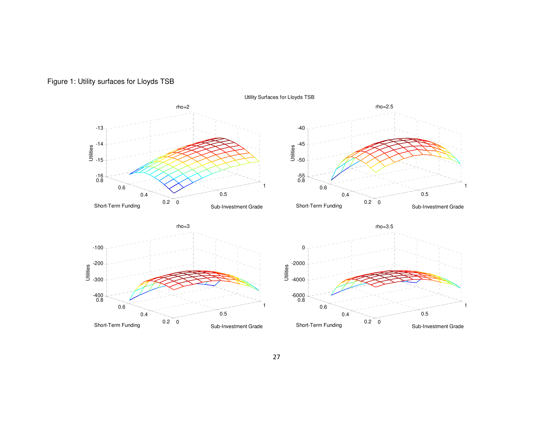
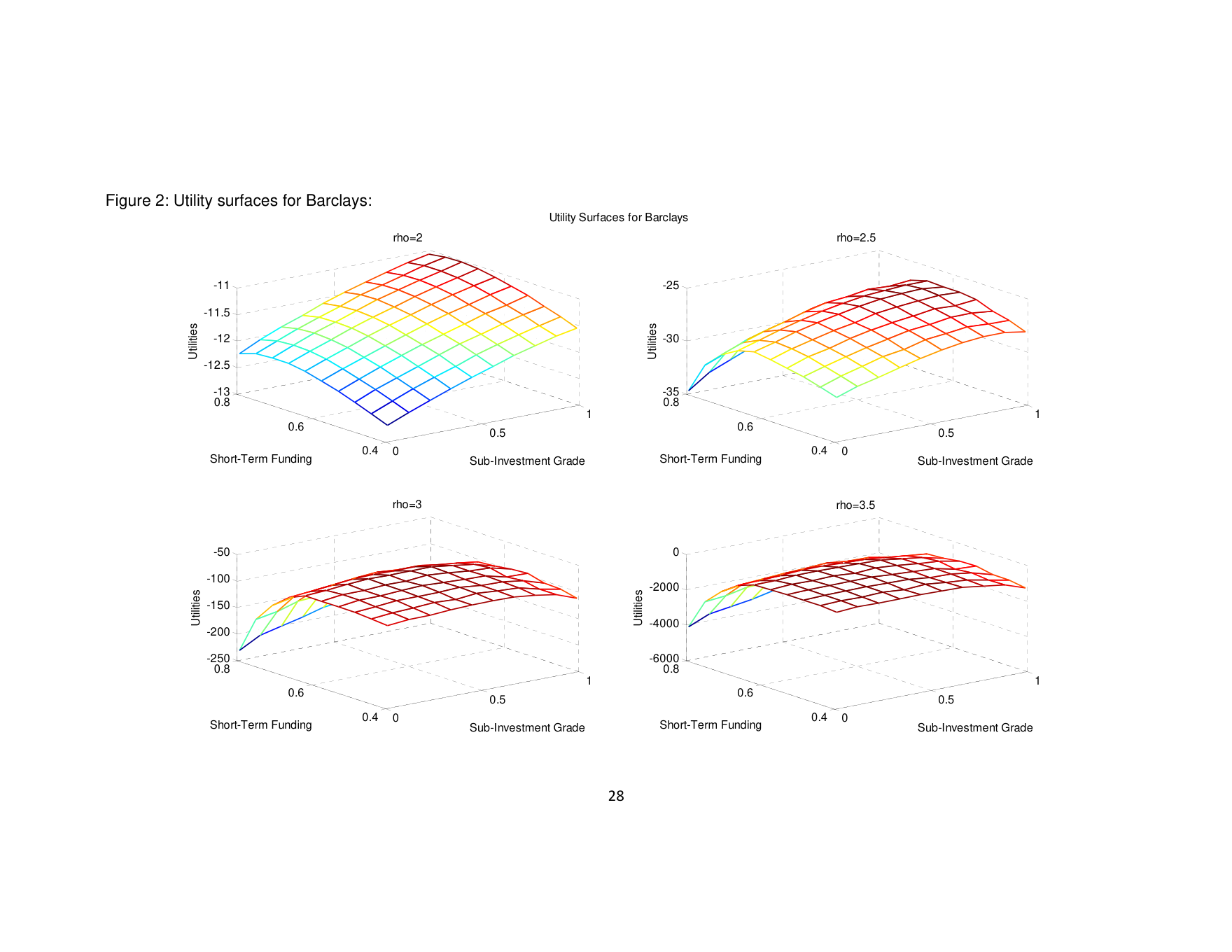
The results of our analysis are shown in a series of tables and charts. To begin with, one may observe in Figures 1 and 2 plots of the utility surfaces for each of the two large banks we analyze. Recall that these utility surfaces are plotted above a set of two dimensional grid points corresponding to different splits of the credit portfolio between investment grade and sub-investment grade and of non-equity liabilities between short (less than or equal to one year) and long funding. Hence, the axes of the plots consist of fractions of the credit portfolios in investment and non-investment grade categories and fractions of non-equity liabilities in the short funding category.
In simulating the model, we seek to find utility function parameters A and ρ that imply that the bank’s choices of portfolio and funding are close to those actually observed. In fact, we set A to a value of 0.001 (which retains a reasonable degree of curvature in the utility surface in the region of the banks’ actual choices, and then vary ρ which as noted above is asymptotically (as A grows large) equal to the Coefficient of Relative Risk Aversion.
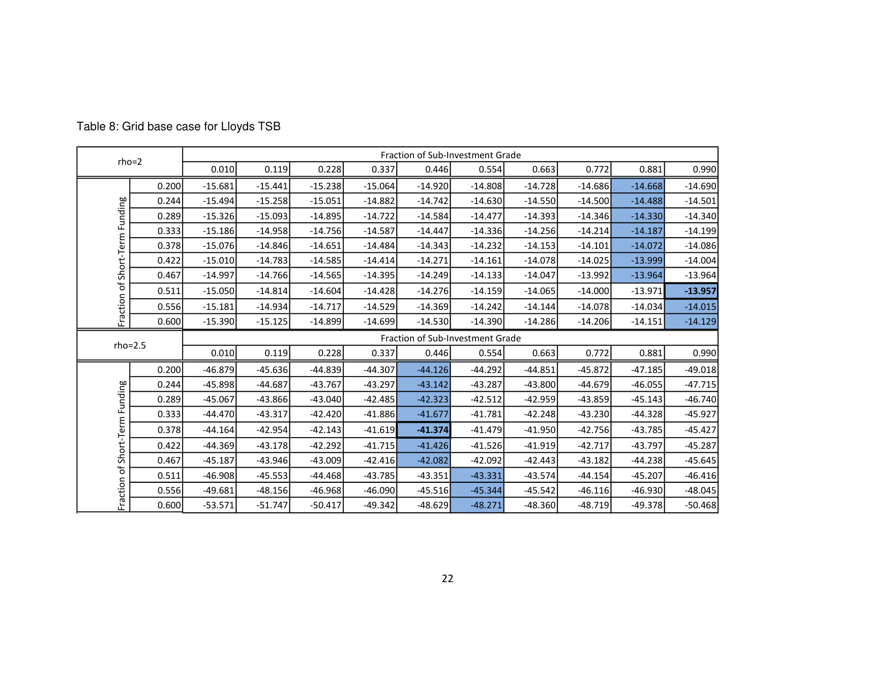
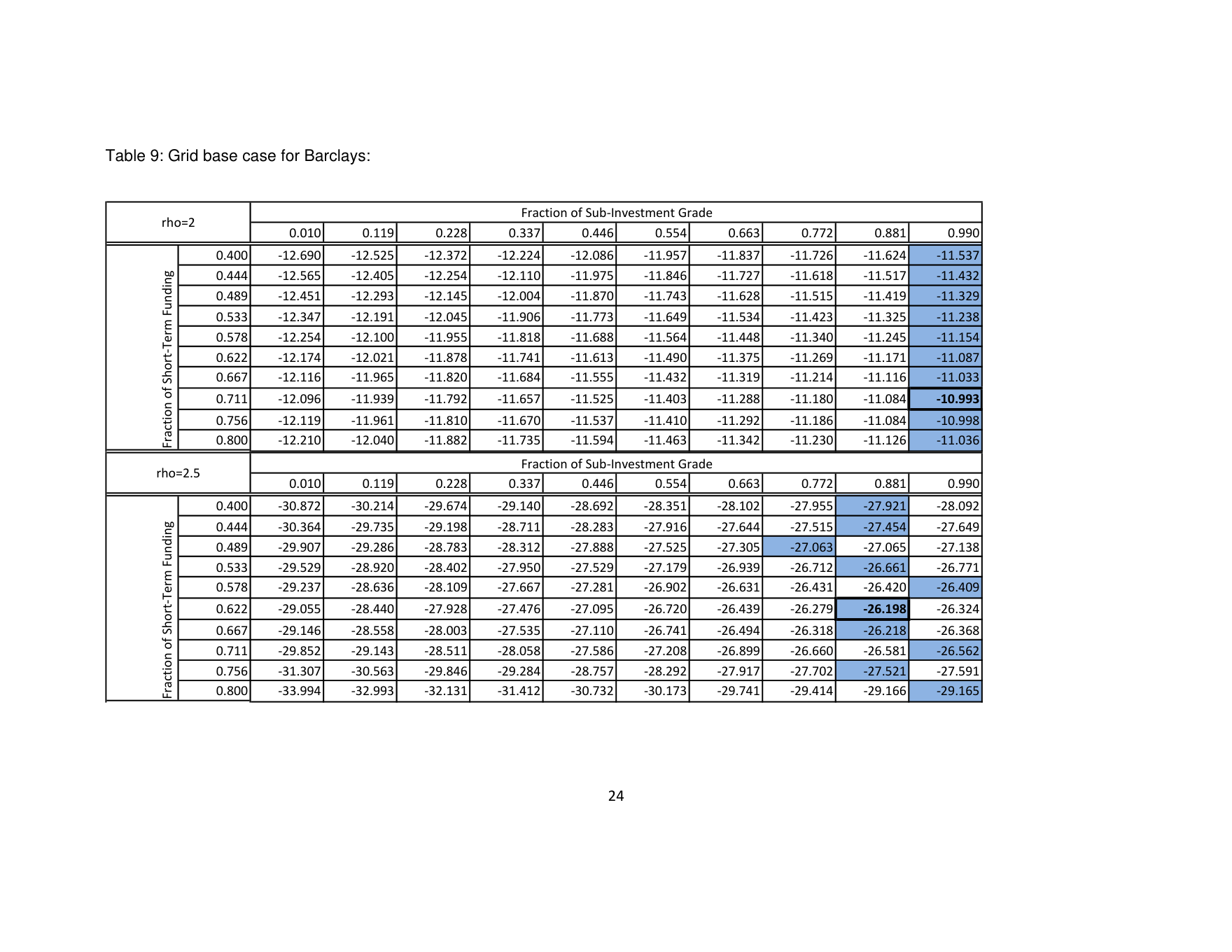
Tables 8 and 9 show the same information as that displayed in the utility surface plots. Viewing the information in tabular form, one may see more easily where in the grid the maximum utility levels are located. We provide tables for different levels of risk aversion (i.e., different levels of ρ) for both LloydsTSB and Barclays.
Tables 8 and 9 show that as risk aversion increases, the expected change occurs in the location of the maximum in that both banks wish to hold a reduced amount of the sub-investment grade portfolio and also wish to employ less short-term funding. The optimal choices are quite sensitive to the level of risk aversion in that different levels of ρ correspond to very different splits in the credit portfolio between investment and sub-investment grade.
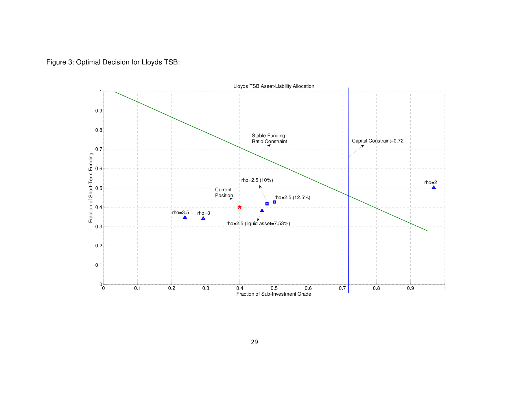
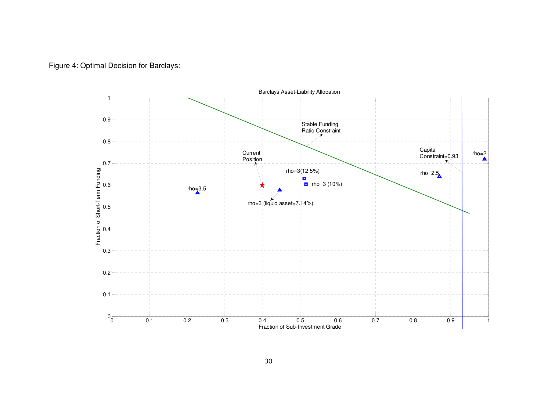
The most important results of our calculations appear in Figures 3 and 4. These two figures (one for each of the two banks we study) superimpose on the grid of asset and funding choices the locations of optimal asset and liability allocations under different assumptions, comparing these with the actual splits observed in the bank data at end 2009.
The figures also show the location of the constraints on bank decisions imposed by
(i) the Basel II capital requirements and (ii) the stable funding liquidity requirements proposed by BCBS (2009).
To explain these, note that the bank’s available equity capital has been fixed at the level observed in end 2009 data. If one calculates the capital required by Basel II using the usual capital charge formulae, certain points in the grid then prove infeasible (since they infringe the Basel minimum). Since funding does not affect the capital calculation, the capital constraint shown in Figures 3 and 4 consists of a vertical line.
On the other hand, the stable funding requirement of BCBS (2009) depends both on funding and to an extent on the ratings of assets. The latter dependence comes from the fact that some high credit quality corporate exposures bear somewhat low weights in the calculation of assets that must be covered by stable funding. Under stylized assumptions about how the rated exposures in the banks’ credit books break down between negotiable bonds and illiquid loans, we derive a restriction which appears as a downward sloping line in Figures 3 and 4.
A ρ value of 2.5 for LloydsTSB and 3 for Barclays implies asset and funding breakdowns similar to those observed. As may be observed from the figures, both LloydsTSB and Barclays lie some way below and to the left of the capital and stable funding constraints. This may reflect the fact that in the current environment, banks have adopted relatively defensive portfolios. (The conclusion also reflects the assumption we have made in parameterizing the model that capital on trading book equals 4% of trading book assets.)
The results show that increasing the holdings of liquid assets implies for both banks an increase in short-term financing. This may reflect the fact that the liquid assets we assume are short-term, default free assets such as Treasury bills and central bank deposits. If the liquid assets involved were longer maturity Treasury securities, the substitution effect would be attenuated or even reversed.
We also find that introducing higher liquid assets increases the share of subinvestment grade credit assets in the banks’ assets. As one might expect, in this riskless liquid assets prove to be closer substitutes for investment grade than subinvestment grade exposures. Potentially, one could experiment with other types of liquid assets such as high credit quality corporate bonds or long maturity sovereign bonds.
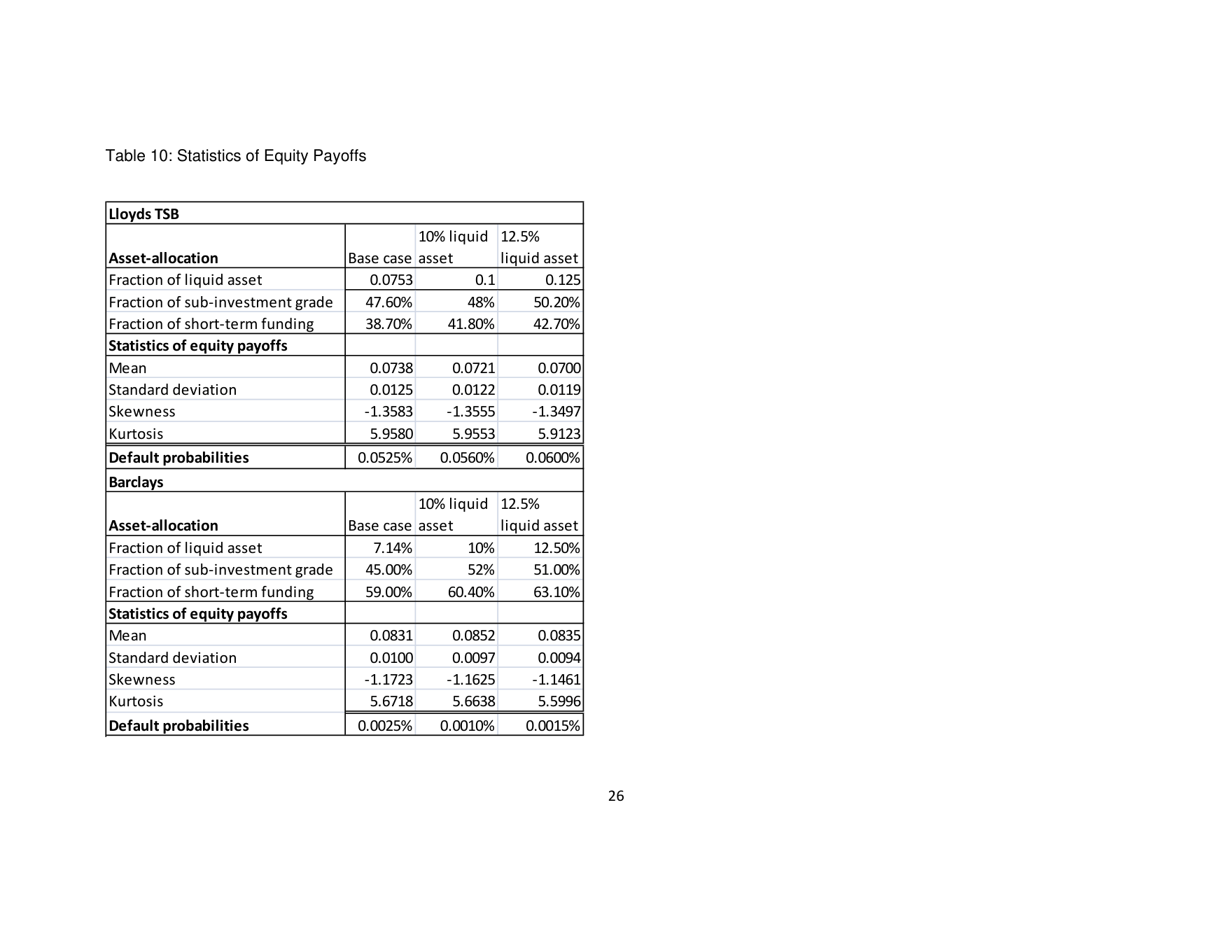
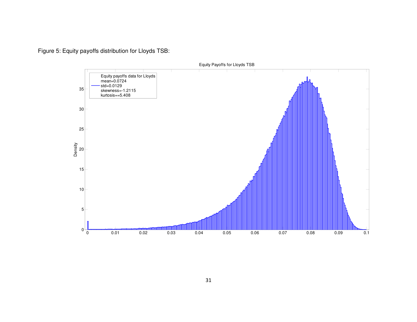
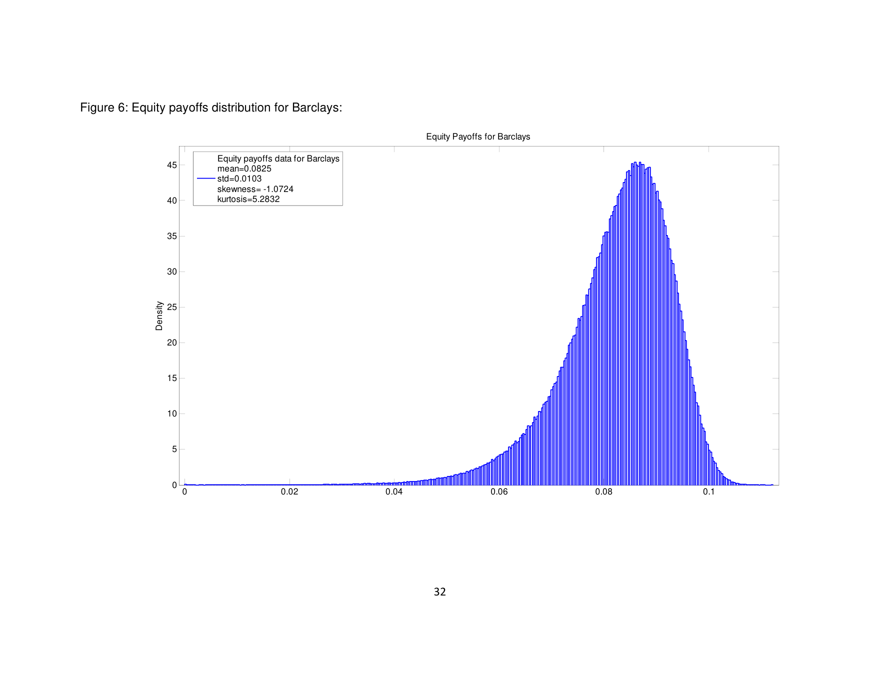
Finally, Table 10 shows statistics of the equity payoffs for the two banks under different assumptions about required liquid assets. Increasing liquid assets for both Lloyds TSB and Barclays reduces risk as measured by the volatility, skewness and kurtosis of the equity payoff. However, in the case of Lloyds TSB, increasing liquid assets reduces the bank’s mean payoff and hence slightly increases the bank’s default probability. In the case of Barclays, the impact on the mean payoff is complex in that it is first rises and then falls as the fraction of liquid assets is increased. Again though, this has an impact on the default probability as this first falls and then rises. The Barclays results underline the complexity of comparative statics for net bank balance sheets when asset-liability substitution effects are taken into account.
5. Conclusion
This paper shows, through a microeconomic analysis, how bank’s optimal choices of assets and liabilities may be affected by a new set of regulatory requirements involving obligations to hold liquid assets and to maintain a balance of stable funding versus illiquid assets.
We formulate a simulation model of bank equity payoffs employing industry standard approaches to modeling credit portfolios and term structures. We build into the model roll-over re-financing costs by making spreads on short-term funding a function of the bank’s rating.
We find that the stable funding requirements appear not to bind for the two large UK banks we examine. When the banks are required to hold additional liquid assets, this induces an increase in short-term funding as one might expect a priori but also increases the banks’ willingness to hold sub-investment grade assets.
References
Acharya, V. V., Shin, H. S. and Yorulmazer, T., 2007, "Fire Sales, Foreign Entry and Bank Liquidity,” CEPR Discussion Papers: 6309.
Acharya, V. V. and Viswanathan, S., 2008, "Moral Hazard, Collateral and Liquidity,” CEPR Discussion Papers: 6630.
Adrian, T. and Shin, H. S., 2008, "Liquidity and Leverage,” Federal Reserve Bank of New York, Staff Reports: 328.
Allen, F. and Gale, D., 1994, "Limited Market Participation and Volatility of Asset Prices,” American Economic Review, 84, 933-955.
Amihud, Yakov, and Haim Mendelson, 1986, “Asset pricing and the bid-ask spread,” Journal of Financial Economics, 17, 223-249.
Amihud, Yakov, and Haim Mendelson, 1991, “Liquidity, maturity, and the yields on US Treasury securities,” Journal of Finance, September, 1441-1426.
Barrell, Ray, E. Philip Davis, Tatiana Fic, Dawn Holland, Simon Kirby and Iana Liadze, 2009, “Optimal regulation of bank capital and liquidity: how to calibrate new international standards,” FSA Occasional Paper 38, July
Basel Committee on Banking Supervision (2009) International framework for liquidity risk measurement, standards and monitoring, Consultative Document, Bank for International Settlements, Basel, December
Bhatia, Mickey, Christoher C. Finger and Greg M. Gupton (1997) "Creditmetrics: Technical Document,” J.P. Morgan, New York
Blum, Jürg (1999) “Do capital adequacy requirements reduce risks in banking?” Journal of Banking and Finance, 23(5) May 755-771
Brace, A., D. Gatarek and M. Musiela (1997) “The Market Model of Interest Rate Dynamics,” Mathematical Finance, 7, 2, 127-55
Brunnermeier, Markus K (2009) “Deciphering the Liquidity and Credit Crunch 2007- 08,” Journal of Economic Perspectives.
Brunnermeier, M., and Pedersen, L.H., 2008, “Market Liquidity and Funding Liquidity,” working paper, Princeton University.
Bryant, J., 1980, “A Model of Reserves, Bank Runs, and Deposit Insurance,” Journal of Banking and Finance, 4, 335-344.
Calem, Paul and Rafael Rob (1999) “The Impact of Capital-Based Regulation on Bank Risk-Taking” Journal of Financial Intermediation 8, 317–352
Chen, L., Lesmond, D. and Wei, J, 2007, “Corporate Yield Spreads and Bond Liquidity,” Journal of Finance, 62, 119-149.
De Jong, F. and Driessen, J., 2006, "Liquidity Risk Premia in Corporate Bond Markets," working paper, University of Amsterdam.
Delianedis, G., Geske, R. , 2002, “The components of corporate credit spreads: default, recovery, tax, jumps, liquidity, and market factors,” working paper, UCLA: Anderson Graduate School of Management, Finance Department.
Diamond, Douglas W., and Philip H. Dybvig, 1983, Bank runs, deposit insurance, and liquidity, Journal of Political Economy 91, 401–419.
Diamond, Douglas W., and Raghuram G. Rajan. 2005. “Liquidity Shortage and Banking Crisis.” Journal of Finance, 60(2): 615–647.
Dow, J., 2004, “Is Liquidity Self-Fulfilling?” Journal of Business, 77, 895-908.
Elton, E., and T.C. Green (1998), “Tax and Liquidity Effects in Pricing Government Bonds,” Journal of Finance, 53, 5, 1533-1562.
Financial Services Authority (2008) Strengthening Liquidity Standards, Consultation Paper 08/22, December
Financial Service Authority (2009) “A regulatory response to the global banking crisis: systemically important banks and assessing the cumulative impact,” Turner Review Conference Discussion Paper, October
Goldstein, Itay and Ady Pauzer (2005) “Demand–Deposit Contracts and the Probability of Bank Runs,” Journal of Finance, 60, 3, June, 1293-1327.
Gorton, G. and Pennacchi, G., 1990, " Financial Intermediaries and Liquidity Creation," Journal of Finance, 45, 49-71.
Heath, D., R.A. Jarrow and A. Morton (1992) “Bond pricing and the term structure of interest rates: a new methodology,” Econometrica, 60, 1, 77-105
Houweling, P., Mentink, A. and Vorst, T. (2005), “Comparing possible proxies of corporate bond liquidity,” Journal of Banking & Finance, 29, 6, 1331-1358.
Kim, D., and A. M. Santomero (1988) “Risk in banking and capital regulation,” Journal of Finance 43, 1219-1233
Koehn, M., and A. M. Santomero (1980) “Regulation of bank capital and portfolio risk,” Journal of Finance 35, 1235-1250
Krishnamurthy, A. (2002), “The bond/old-bond spread” , Journal of Financial Economics, 66, 463-506
Lamb, R., and W.Perraudin (2008). “Dynamic Default Rate,” working paper, Imperial College, London.
Longstaff, F. A., Mithal, S. and Neis, E., 2005, "Corporate Yield Spreads: Default Risk or Liquidity? New Evidence from the Credit Default Swap Market,” Journal of Finance, 60, 2213-2253.
Parlour, C. and Plantin, G., 2008, “Loan Sales and Relationship Banking,” Journal of Finance, 63, 1291-1314.
Pástor, L. and Stambaugh, R. F., 2003, "Liquidity Risk and Expected Stock Returns," Journal of Political Economy, 111, 642-85
Perraudin, W. R. M., and Taylor, A. P., 2007, "Liquidity, Bond Market Spreads and Conditional Risk Premia," working paper Imperial College, London.
Plantin, G., 2008, “Learning by holding and liquidity,” Review of Economic Studies, (forthcoming).
Shin, H., 2006, “Disclosure Risk and Price Drift,” Journal of Accounting Research, 44, 351-379.
Shin, H., 2008, “Risk and Liquidity in a System Context,” Journal of Financial Intermediation, 17, 315-329.
Silber, W. L., 1991, “Discounts on restricted stock: The impact of illiquidity on stock prices,” Financial Analysts Journal, July-August, 60.
Taylor, John B. and John C. Williams, 2008, “A Black Swan in the Money Market,” National Bureau of Economic Research, Inc, NBER Working Papers: 13943
Tables and Charts
| Lloyds TSB | Barclays | |
|---|---|---|
| Assets | 1.000 | 1.000 |
| Cash | 0.075 | 0.071 |
| Trading book excluding cash | 0.040 | 0.570 |
| Banking book excluding cash | 0.960 | 0.430 |
| Liabilities | 1.000 | 1.000 |
| Equity | 0.041 | 0.042 |
| Funding | 0.959 | 0.959 |
| Short term funding | 0.384 | 0.575 |
| Long term funding | 0.576 | 0.383 |
| Rating breakdown of IRB business | ||
| AA | 8.8% | 20.9% |
| A | 21.7% | 9.2% |
| BBB | 30.4% | 30.2% |
| BB | 26.3% | 30.3% |
| B | 10.6% | 6.1% |
| CCC | 2.2% | 3.4% |
| Investment grade | 60.9% | 60.2% |
| Non-investment grade | 39.1% | 39.8% |
| Lloyds TSB | Barclays | |
|---|---|---|
| Assets | ||
| Trading book excluding cash | ||
| Mean excess return | 4.0% | 4.0% |
| Volatility of excess return | 0.5% | 0.5% |
| Mean dividend rate | 1.0% | 1.0% |
| Banking book excluding cash | ||
| Risk factor weights | ||
| Industry/country ratio | 1.0 | 1.0 |
| Indiosyncratic weight | 0.2 | 0.2 |
| Recovery rate | 0.6 | 0.6 |
| Coupon Rate | ||
| AA | 5.0% | 5.0% |
| A | 5.7% | 5.7% |
| BBB | 6.2% | 6.2% |
| BB | 6.5% | 6.5% |
| B | 6.7% | 6.7% |
| CCC | 7.0% | 7.0% |
| Spread refinancing cost factor weights | ||
| A | 0.6 | 0.6 |
| BB | 0.2 | 0.2 |
| CCC | 0.2 | 0.2 |
| Liabilities | ||
| Long term funding | ||
| Yield | 4.0% | 4.0% |
| Short term funding | ||
| Spread over reference rate | 50bps | 50bps |
| Rating | Default | Spread |
|---|---|---|
| Classes | Probatility (%) | (%) |
| AAA | 0.00 | 0.00 |
| AA+ | 0.00 | 0.00 |
| AA | 0.01 | 0.00 |
| AA- | 0.04 | 0.02 |
| A+ | 0.05 | 0.03 |
| A | 0.05 | 0.03 |
| A- | 0.05 | 0.03 |
| BBB+ | 0.14 | 0.07 |
| BBB | 0.18 | 0.09 |
| BBB- | 0.35 | 0.18 |
| BB+ | 0.76 | 0.38 |
| BB | 0.84 | 0.42 |
| BB- | 1.97 | 0.99 |
| B+ | 3.26 | 1.64 |
| B | 5.20 | 2.63 |
| B- | 10.06 | 5.16 |
| CCC | 19.81 | 10.43 |
| Trading | |||||||
|---|---|---|---|---|---|---|---|
| Book | AA | A | BBB | BB | B | CCC | |
| Trading Book | 1.00 | 0.30 | 0.30 | 0.30 | 0.30 | 0.30 | 0.30 |
| AA | 0.30 | 1.00 | 0.95 | 0.90 | 0.85 | 0.80 | 0.75 |
| A | 0.30 | 0.95 | 1.00 | 0.85 | 0.80 | 0.75 | 0.70 |
| BBB | 0.30 | 0.90 | 0.85 | 1.00 | 0.75 | 0.70 | 0.65 |
| BB | 0.30 | 0.85 | 0.80 | 0.75 | 1.00 | 0.65 | 0.60 |
| B | 0.30 | 0.80 | 0.75 | 0.70 | 0.65 | 1.00 | 0.55 |
| CCC | 0.30 | 0.75 | 0.70 | 0.65 | 0.60 | 0.55 | 1.00 |
| Maturity | Sterling |
|---|---|
| 3-month | 0.0054 |
| 1-yr | 0.0066 |
| 1-yr | 0.0097 |
| 3-yr | 0.0179 |
| (0-0.25 year) | 0.2099 | 0.2284 | 0.0871 | 0.0473 |
|---|---|---|---|---|
| (0.25-1 year) | 0.2284 | 0.3121 | 0.1267 | 0.0708 |
| (1-3 years) | 0.0871 | 0.1267 | 0.0751 | 0.0436 |
| (3-5 years) | 0.0473 | 0.0708 | 0.0436 | 0.0297 |