

This report analyses the ratings and capital adequacy of the two sovereign lending organisations within the World Bank Group, the International Bank for Reconstruction and Development (IBRD) and the International Development Association (IDA). Specifically, we quantify the headroom available to these organisations to expand development lending. The analyses are performed using public data obtained from their financial statements and the annual rating assessments of the three global rating agencies, Standard & Poor’s, Moody’s, and Fitch.
Executive Summary
This report analyses the ratings and capital adequacy of the two sovereign lending organisations within the World Bank Group, the International Bank for Reconstruction and Development (IBRD) and the International Development Association (IDA). Specifically, we quantify the headroom available to these organisations to expand development lending. The analyses are performed using public data obtained from their financial statements and the annual rating assessments of the three global rating agencies, Standard & Poor’s, Moody’s, and Fitch.
IBRD and IDA face several constraints in managing their balance sheets. These include:
1. The ratings they receive from the rating agencies, more specifically that no downgrade occur in the organisation’s AAA rating.
2. The constraint of internal MDB Capital Adequacy Frameworks which generally require that Capital Resources exceed Capital Required (so the Capital Adequacy Ratio equal to the ratio of Capital Resources to Capital Required exceed unity plus perhaps a buffer). If the organisations choose to transfer risk, they also face:
3. The constraints provided by the pricing that the market requires to supply insurance.
4. If tranched risk transfer is employed, the approach the rating agencies take to evaluating portions of the risk.
Finally, each of the organisations faces one additional constraint:
5. IBRD is constrained by the Statutory Lending Limit (SLL) included in its articles of agreement. (IDA has no corresponding SLL.)
6. IDA is constrained by the need to sustain its business model as a concessional lender. An institution that lends $100 at a zero-interest rate and is not obliged to pay a dividend, (so long as it covers its costs through fees), can sustainably relend the money when it is repaid, again for a zero-interest rate. In this case, for the institution is to operate sustainably, its lending volume is effectively constrained by the size of its equity. We term this constraint the Sustainable Concessional Lending Limit (SCLL).
These constraints are opaque for all but a few specialists within the institutions themselves. This study aims to clarify the nature of the constraints and to examine the room available to the two organisations to increase lending before one or other constraint binds.
To achieve this, we, first, replicate the rating analysis that the two institutions receive from the three global rating agencies. We compute the quantitative elements in the agency scorecards and analyse how judgmental components are likely to respond to changes in the scale of lending.
Second, using public data on the institutions’ sovereign lending portfolios, we calculate the credit risk capital that the institutions may conservatively choose to hold. While credit risk capital is only part of the total Economic Capital (EC) (the latter should also cover market, operational and other risks), for sovereign focussed MDBs, credit risk capital is likely to be between 80 and 90% of total EC. Hence, our calculations will provide a reasonably accurate view of the institutions’ Capital Adequacy Ratios (i.e., capital available divided by capital required).
Third, we calculate the amounts of fully concessional and fully non-concessional loans that are equivalent to a dollar of blended lending for IDA. We argue that the non-concessional lending is unconstrained since the institution’s available capital is sufficient to borrow extensively in capital markets. The sum of IDA’s fully concessional lending and the concessional component of its blended loans is less than its capital which creates room to lend more either through more concessional or more blended loans.
Fourth, we analyse the scope for the institutions to transfer risk on their sovereign to public donors or to the private market. In our study, we focus on synthetic securitisations in which the institution retains a junior (sized to cover the Expected Loss on the securitised portfolio) and a thick senior tranche. In this context, a key issue is the rating that the rating agencies assign to the retained senior tranche because this affects the efficiency of the risk transfer. In the light of these factors, we compute the additional lending that the institutions could achieve and the different risk transfers.
Our findings for IBRD are as follows.
x For IBRD, the constraints of maintaining a AAA rating and maintaining capital resources greater than required Economic Capital are less constraining that the Statutory Lending Limit (SLL). The SLL binds when the portfolio of DRAs and Treasury assets has expanded by no more than 45%. IBRD has already raised the possibility to its Board of Directors that its SLL be abolished. x The IBRD could boost its Development Related Asset (DRA) lending and Treasury assets by around 71% before its Moody’s rating is downgraded. Fitch would downgrade the IBRD at 101%. The Standard & Poor’s rating is much less constraining and would only be downgraded after more an expansion of 152%. x The constraint that the Capital Adequacy Ratio (CAR) exceed unity is less constraining for IBRD than the ‘no rating downgrade’ constraint, in that exposure could increase by 147% before the CAR equals unity. Of course, evaluating the CAR depends on how Economic Capital (EC) is calculated. In this study, we have implemented an industry standard Credit Portfolio Model (CPM), calibrated it based on commonly applied techniques and provided sensitivity analysis. We have also assumed that the net contribution of non-DRA-loan-related components of EC amount to no more than 10% of DRA-loanrelated EC. This is true of some other sovereign focussed MDBs. Finally, we have added a buffer of 10% to the DRA-credit-related capital estimate generated by the CPM we employ. Again, we have observed other MDBs that work with buffers of the order of 10% in computing their CAR.
Our analysis of IDA results in the following findings. x We allow for the presence on its balance sheet of highly concessional loans. These are booked at par (justified by the fact that IDA does not pay dividends) but the value of these loans would have to written down if IDA were insolvent. If the value of loans were adjusted, IDA’s equity would be correspondingly lower. Even though the rating agencies do not adjust its equity for the subsidy value of its loans, IDA, in its internal capital adequacy assessments chooses to include an adjustment. It applies this to the required capital resources rather than by discounting loan values which appears to be more natural. In the CAR analysis we perform for IDA, we follow the latter approach by calculating and subtracting from assets the value of the subsidy element in IDA’s loans. x We find that the ratings constraint for IDA hardly binds at all. Substantial expansion in DRAs and Treasury assets, of around 200%, would be necessary before any downgrade occurs. Even larger increases in assets would be required before a CAR constraint were breached. The expanded DRAs in question would consist either of non-concessional loans or concessional loans for which IDA finds donor governments willing to cover the subsidy component. x While IDA could borrow extensively, a conclusion that it can boost its concessional lending extensively would be misplaced. The institution’s non-binding rating constraint and very high CAR mean that it has plenty of scope to lend more on a non-concessional basis. But IDA and most of its stakeholders are clear that it should remain a concessional lender. Such a lender faces the additional constraint that managing its balance sheet sustainably permits it only to offer fully concessional, zero-interest-rate loans up to a ceiling of its equity (assuming it can cover its costs from fees). As we show in the study, there remains some unexploited headroom in IDA’s lending because only part of its existing loan book is fully concessional while a large fraction is 'blended’ (meaning partially concessional but not zerointerest-rate) and a small amount is non-concessional. This lending profile means that some additional lending headroom remains. This we compute to equal 15% or 12% of its total loan book par value depending on whether it chooses to boost concessional or blended lending. (Note that in this analysis, we are not assuming any additional donor willingness to cover the concessional element in IDA lending.)
Figure ES1 summarises the constraints on lending implied by the three primary constraints on lending by IBRD and IDA that are investigated in this study. For IBRD, the tightest constraint is the Statutory Lending Limit (SLL) which binds after net loans and guarantees have expanded by 45%. The rating constraint binds for IBRD when lending and guarantees have increased by 71%. This binds when the Moody’s rating is downgraded from Aaa. The Fitch rating is downgrade shortly thereafter whereas there is plenty of room for IBRD to expand lending before the Standard & Poor’s rating is downgraded. The Economic Capital (EC) constraint (i.e., that the Capital Adequacy Ratio (CAR) (allowing for a buffer of 10% exceeds unity) is only breached after a substantial increase in exposure (and, hence, lending) of 147%.
The precise values of these calculations are, of course, subject to assumptions. The rating calculations presume some deterioration in the qualitative questions that the rating agencies include in their rating evaluations. For Moody’s in particular, the judgmental elements are reduced to precise questions that place the MDB in one or other of several discrete categories. Determining the expansion in lending but they might shift to more negative categories that triggers a deterioration in these judgmental scorings in turn requires that we make a judgment or assumption. Similarly, in the EC constraint calculations, many aspects of the Credit Portfolio Model (CPM) employed in the calculations might be questioned. We have tried several reasonable sensitivity analyses and adopted reasonable assumptions with some conservative elements.
Figure ES1: Summary of Lending Headroom
Panel a) IBRD Panel b) IDA
ϭϲϬй ϭϰϳй
ϭϰϬй
ϭϮϬй
ϭϬϬй
ϴϬй ϳϭй
ϲϬй ϰϱй
ϰϬй
ϮϬй
Ϭй ^>> ZĂƚŝŶŐ
Note: The red bars illustrate, for IBRD and IDA, the headroom for additional non-concessional lending in percent of current net lending and guarantees implied by the three sources of constraint, namely Statutory Lending Limit (indicated by ‘SLL’), the requirement that the AAA-ratings of all three global rating agencies be maintained (labelled ‘Rating’) and that the Capital Adequacy Ratio (equal to capital resources (paid in equity and reserves) divided by capital required (Economic Capital plus a 10% buffer)) exceeds unity. IDA has no SLL constraint. In computing CARs for IDA, we have followed a conservative approach, comparable to IDA’s internal risk management methodology, of adjusting capital resources downwards to allow for the value of the subsidy element in IDA’s loans. More information about the computations may be found in the sister technical paper, Risk Control (2023). The dark blue bars show headroom as a percentage of IDA total lending (relative to the SCLL) if it expands its lending using particular, subsidised loan instruments (CLs or BLs). SCLL denotes Sustainable Concessional Lending Limit, NCL denotes Non-Concessional Loan, CL denotes Concessional Loan, RL denotes Regular Loan and BL denotes Blended Loan. Note that because of the differences in the way these constraints are applied, the rating headroom (71% for IBRD) is expressed in terms of outstanding loans whereas the EC headroom (147% for IBRD) is expressed in terms of outstanding loans plus 50% of undisbursed commitments.
Panel b) in Figure ES1 shows the scope for IDA to expand lending. The red bars show the headroom to increase lending implied by the rating and EC constraints. These suggest the scope to expand IDA’s balance sheet is very great. The figures are only relevant, however, if the expansion were to involve non-concessional lending. The analysis demonstrates that IDA has a sufficiently large capital cushion that it could readily borrow more in the bond market and lend it out so long as the cost of borrowing could be remunerated (i.e., the lending be nonconcessional). Borrowers would still benefit from such loans in that the costs would be low compared to those of borrowing in the market themselves, but they would have to pay a risk-free interest rate plus a credit spread to cover Expected and Unexpected Losses.
IDA and its stakeholders, however, are clear that the institution will remain primarily a concessional lender (even though it is moving towards a ‘hybrid’ approach that includes some blended loans and even a small amount of non-concessional lending). Unless IDA can find additional donors, willing to bear the cost of the subsidy element in additional concessional lending, it will remain constrained by what we refer to above as the Sustainable Concessional Lending Limit (SCLL), i.e., the constraint that fully concessional (zero-interest-rate) lending plus the fraction of blended loans that amounts to fully concessional loans be less than the organisation’s equity capital. On this basis, we are still able to identify some headroom in IDA’s current lending. This appears as the blue bars in Figure ES1 which show that IDA could boost its blended or concessional loans by an amount equal to 15% or 12%, respectively, of IDA’s total loan par value.
We assess the potential for IBRD and IDA to engage in risk transfer outside the World Bank Group, buying credit protection from external entities that might consist of donor governments, private sector entities or some combination of the two. We compute the reduction in economic capital (EC) for IBRD and IDA when they securitise their respective portfolios A and B. We find that securitisation reduces the EC substantially if the securitised portfolio is riskier. for IBRD the reduction in EC is 12% for portfolio A and 18% for portfolio B. For IDA, the reduction in EC turns out to be 12% for both portfolio A and B (see Table 7.4).
These findings imply that risk transfer offers an effective safety valve in relaxing some of the lending constraints that IBRD and IDA may face. But there are some significant obstacles here. For IBRD, the tightest constraint is the SLL. If the SLL were relaxed (as has been proposed by IBRD), the first constraint to bind would be that associated with a downgrade in the Moody’s rating. But, when lending expands, the Moody’s rating is affected by a deterioration in both the leverage ratio and the contractual support ratio. This would not be much improved by a securitisation that left IBRD with a thick retained senior tranche.
1. Introduction
Multilateral Development Banks (MDBs) play a key role in financing economic growth in Emerging Market and Developing Economies (EMDEs). An International Monetary Fund study published in 2019 (see IMF (2019)) calculated that an additional US$2.6 trillion of spending per annum until 2030 was required if Emerging Market Economies (EMEs) and Low-Income Countries (LICs) were to meet the requirements of the Sustainable Development Goals (SDGs) in five key areas (education, health, roads, electricity, and water and sanitation).
The current climate emergency further boosts the investment needs of EMDES. An Independent High-Level Expert Group on Climate Finance (LSE (2022)) found that EMDEs other than China must spend US$2.4 trillion per year by 2030 to achieve the climate goals agreed upon in Paris Agreement across all dimensions.
The report of the Panel on Capital Adequacy Frameworks published in June 2022 (see CAF Panel (2022)) proposes steps that MDBs might take that would permit a significant expansion in their lending. MDBs are considering the feasibility of the Panel’s proposals. At the same time, MDB shareholders, primarily sovereign governments of both donor and borrower Member Countries (MCs), are examining what they could do, either through direct support to MDB lending or indirectly through their governance of MDBs, to advance the CAF Panel’s agenda.
This study aims to contribute to the debate initiated by the CAF Panel report by examining in detail the capital adequacy of two major MDBs, namely the International Bank for Reconstruction and Development (IBRD) and the International Development Association (IDA). The two institutions represent the sovereign lending focussed members of the World Bank Group. Collectively, they contribute a major fraction of total development lending by MDBs. Through their influential position among MDBs, they can also influence the actions of other institutions.
The analyses we perform are based on public data. Understanding the finances of an MDB from the outside has its challenges. For MDBs, there is no equivalent to the Pillar 3 reports issued by large commercial banks. Individual MDBs provide risk management sections in their financial statements but details are limited. An important public source of information is ratings agency reports on MDBs. But agency evaluations contain judgmental elements and are not fully transparent.
Despite these obstacles, some major MDBs are reasonably straightforward to analyse from the outside since their exposures primarily consist of sovereign loans, information on which is published in their annual reports. The IBRD and IDA correspond to this pattern. Like many MDBs, the two institutions have very low appetite for market or operational risk and hold high quality and short-dated Treasury assets. Hence, most of their risk and, therefore, Economic Capital reflects their sovereign lending.
To shed light on the ratings and capital adequacy of IBRD and IDA and, therefore, to infer the scope they have for additional lending, we perform three exercises.
1. We investigate the rating agency assessments of IBRD and IDA through a careful analysis of the methodologies employed by the three global agencies, Standard & Poor’s, Moody’s and Fitch. We calculate the point at which the ratings assigned by the agencies change if the IBRD and IDA progressively scale up their Development Related Assets (DRAs) and Other Assets (primarily Treasury assets) without a change in their equity resources. This analysis draws on a precise replication of the decision-trees employed by the rating agencies.
The agencies apply methodologies that are to varying degrees precise and publicly disclosed. All three agencies rely on a combination of quantified indicators and qualitative judgments. In the case of Moody’s, the judgments are formulated as questions that appear in the methodology documents. For others, most notably Fitch, the judgmental elements are less precisely expressed in the published methodologies, so we have endeavoured to express them as questions.
The analysis shows how different elements of the scorecards (or ‘decision trees’) lead to a change in rating as the lending and Treasury assets expand proportionally. In the exercise, we allow for deterioration in the answers to the qualitative questions as the balance sheet grows.
2. The second exercise we perform is to implement a set of industry standard Economic Capital (EC) calculations using a ratings-based Credit Portfolio Model (CPM). Much the largest part of the risk faced by MDBs is attributable to credit risk. For a representative MDB other than IBRD and IDA, we believe that the contribution of other risks in Economic Capital calculations is around 10%. Hence, computing the credit risk EC for an MDB tells one a lot about total EC. The model we implement is a ratings-based CPM resembling those employed by (almost all) large commercial banks for Pillar 2 capital calculations and identical in most respects to what we have observed in use in several large MDBs. The model builds on the so-called ‘Ordered Probit’ methodology popularised by JP Morgan and commonly labelled the Creditmetrics approach.
We implement several different calibrations to investigate the model’s sensitivity and the robustness of the conclusions. A key aspect of the calibration is the degree to which sovereign loan Probabilities of Default (PDs) and Loss Given Default (LGD) rates are assumed to reflect Preferred Creditor Treatment (PCT). MDBs benefit from PCT to the extent that they are treated as senior by distressed sovereigns that default on other debt claims. Since sovereigns operate outside any formal, legal insolvency framework, they can choose to default on one creditor’s claims but not another’s. One may observe from historical experience that MDBs enjoy significant de facto seniority even though this is not written into debt contracts. We show, though our calculations, that the magnitude of PCT effects substantially influences any evaluation of the capital adequacy of the IBRD and IDA.
An additional consideration for EC analysis of IDA is the fact that the institution engages in heavily concessional lending. While its loans are booked at par in its balance sheet, their value is in most cases much lower because they bear interest rates much below market rates (and even below the rates that would be fairly priced, allowing for the de facto seniority or Preferred Creditor Treatment (PCT) that IDA enjoys). Lower loan values might then imply reduced equity. IDA’s accounts do not include a loan value adjustment because the loans are assumed to be financed with equity and IDA is not expected to pay dividends on its equity.
While the rating agencies do not adjust IDA’s equity for the lower value of its loan book, IDA itself in its internal risk management chooses to add loan value adjustment to its EC to obtain when it labels its Total Required Resources. This then is compared to its Total Available Resources, i.e., its equity. In our CAR analysis, we perform a detailed calculation of the value of IDA’s loan subsidies. Finding this a more natural approach, we then adjust down equity resources rather than adjusting up required capital.
3. The third exercise we calculate the amounts of fully concessional and fully non-concessional loans that are equivalent to a dollar of blended lending. IDA currently lends an amount approximately equal to its capital, but this lending includes (i) non-concessional loans, (ii) so-called blended loans and (iii) fully concessional (zero-interest-rate) loans. Blended loans have relatively low but still non-zero interest rates.
We argue that the non-concessional lending is unconstrained since the institution’s available capital is sufficient to borrow extensively in capital markets. The sum of IDA’s fully concessional lending and the concessional component of its blended loans is less than its capital which creates room to lend more either through more concessional or more blended loans.
4. The fourth exercise we perform is to consider the feasibility of risk transfer for IBRD and IDA. Specifically, we consider synthetic securitisations of sub-portfolios of these institutions’ sovereign loan books. Key aspects are the prices that the market might set to provide insurance and the ratings that the rating agencies would assign to tranches that the two institutions might retain. The ratings of retained senior tranches matter because they feed back into the agencies’ ratings of the MDBs themselves and, hence, influence the capital efficiency of risk transfer as far as the institutions are concerned.
On the first topic, we employ a pricing approach based on a simple analytical model and calibrated to pool expected losses adjusted for market risk premiums using sovereign bond market data. On the second topic, we assume that the retained senior tranches are rated using a methodology that Standard & Poor’s developed at the request of the African Development Bank (AfDB) for application to the retained senior tranche in the landmark 2019 Room2Run transaction.[1]
From the four analyses just described (of ratings, capital adequacy and risk transfer), we shed light on the headroom available to the IBRD and IDA to expand their lending. In managing their balance sheets, the two institutions face the following constraints:
1. Agency ratings of the MDBs themselves
2. Internal Capital Adequacy Frameworks
3. Rating agency treatment of risk transfers
4. Market pricing of risk transfers
5. For IBRD, there is a fifth constraint, namely the gearing constraint included in its statutes.
6. For IDA, there is an additional constraint, namely the Sustainable Concessional Lending Limit (SCLL).
Through our analyses, we show how and when these constraints would bind if lending were to expand.
The document is organised as follows. Section 2 provides profiles of the two institutions from a financial and risk point of view. This provides important context for what follows. Specifically, we describe the two institutions’ balance sheets and the key risk indicators on which the institutions themselves focus. Section 3 examines the ratings the two institutions receive from the three major rating agencies and investigates how these ratings would be affected by an expansion in lending, accompanied by a proportionate increase in nonloan assets (thereby maintaining liquidity). Section 4 describes a series of capital adequacy calculations for the two institutions based on public data on their sovereign loan books. Section 5 explains the constraint on IDA lending attributable to its use of concessional loans. Section 6 investigates the scope for risk transfer off the balance sheets of the two institutions involving synthetic securitisation of the institutions’ sovereign loans. Section 7 brings together the different analyses of ‘headroom’ and, also, examines the constraint on lending provided by the institutions’ statutory lending limits. Section 8 concludes. A series of appendices provide additional information on technical and data issues.
2. Risk Profile of the Two Institutions
2.1 Indicators
This section presents the financial and risk profiles of the IBRD and IDA. This is important context for the subsequent discussion.
To ‘profile’ the institutions, we focus on a set of publicly available indicators, namely:
1. Balance sheet variables, such as the volume of loans and Treasury assets
2. An externally generated risk indicator, the Risk Adjusted Capital (RAC) ratio employed by Standard & Poor’s
3. The internal ratios that the IBRD and the IDA employ in managing their balance sheet, the equity-toloans ratio, in the case of IBRD, and the Deployable Strategic Capital (DSC) ratio of IDA
4. The country breakdown of the two MDBs’ loan portfolios
2.2 Balance sheet variables
Figure 2.1 presents data on the evolution from 2018 to 2022 of the loans and Treasury assets of the two MDBs. IBRD loans (shown in dark blue in Panel a) have grown by 20% in the period from 2018 to 2022 (from $254bn to $304bn). IDA’s loans have similarly increased by 18% over the same period (from $211bn to $250bn).
The two MDB’s Treasury assets have growth at slower rates over the four-year period, 14% for IBRD and 11% for IDA. To finance the growth, IBRD’s borrowings grew by 13% (from $208bn to $235bn). Starting from a low base, IDA’s borrowings increased by 371% (from $7bn to $33bn), reflecting the institution’s newly adopted strategy of additional debt-financed lending (see IDA (2018)).
In summary, IBRD lending has exhibited steady if slow growth, with a slight acceleration in 2021 followed by a slowing the following year. In real terms, adjusting for US consumer price inflation, IBRD lending is flat. Over the four-year period, IDA loan growth appears to be steady but again it is flat in real terms.
Figure 2.2 shows the evolution over the last four years of the two MDBs’ Total Equity and Callable Capital. The IBRD’s Total Equity grew by 31% over the four-year period from ($42bn to $55bn). The Callable Capital of IBRD increased from $258bn to $287bn, a rise of 11%. IDA’s Total Equity increased by 9% (from $164bn to $179bn). IDA has no Callable Capital.
The sources of growth in IBRD Total Equity may be understood as follows. The percentage increase reflects a mixture of higher retained earnings (unrealized market gains), Accumulated other Comprehensive Income (AOCI)[2] and greater paid in capital. In the period 2020 to 2022, retained earnings generated about $6bn. AOCI increased by $3.3bn over the four-year period to 2022. Paid in capital grew by $4bn over the four-year period to
2022. The increase is attributable to the Transformative Capital Package (see World Bank (2018)) which aims to contribute in total additional paid-in capital of $7.5bn over a five-year period starting in 2018. As we shall see below, the strikingly high growth rate of IBRD’s Total Equity as recorded in its financial statements is not matched by that of the equity aggregate which IBRD uses in its internal capital adequacy policies. Hence, the equity growth has not triggered any expansion in lending targets.
Figure 2.2 underlines the very different structure of the two MDBs’ equity. IBRD has a small paid in equity capital plus reserves (Total Equity) relative to its Callable Capital, while IDA has substantial Total Equity but zero Callable Capital. The high Total Equity levels of IDA are consistent with its status as a concessional lender and grant providing multilateral.
One may compare the structure of IBRD and IDA equity with that of the major regional MDBs, Asian Development Bank (ADB), Inter-American Development Bank (IDB), African Development Bank (AfDB) and European Investment Bank (EIB). For IBRD and IDA, respectively, the ratios of Callable Capital to Total Equity is 5.2 and 0. For the above listed regional MDBs, the ratios (in increasing order) are 2.5 for ADB, 3 for EIB, 4.4 for IADB, and 12.5 for AfDB.
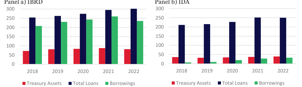
Note: Units are USD billion. The source for Panel a) is IBRD (2022), IBRD (2020) and IBRD & IDA (2018). The source for Panel b) is IDA (2022), IDA (2020) and IBRD & IDA (2018).
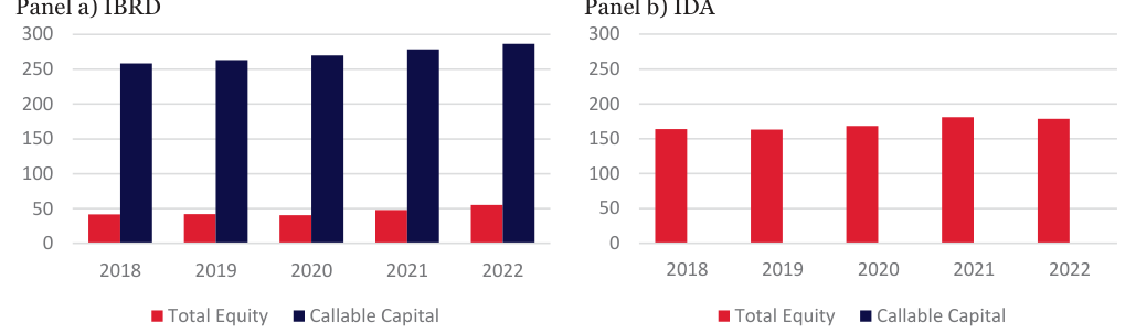
Note: Units are USD billion. The source for Panel a) is IBRD (2022), IBRD (2020) and IBRD & IDA (2018). The source for Panel b) is IDA (2022), IDA (2020) and IBRD & IDA (2018).
2.3 The Standard & Poor’s RAC ratio
One may obtain a perspective on the capital adequacy of IBRD and IDA by considering the Risk Adjusted Capital (RAC) ratio published by Standard & Poor’s for the MDBs that it rates (see Standard & Poor’s (2022a)).
The RAC is the ratio of Total Adjusted Capital (TAC) (as defined by the agency) to Risk Weighted Assets (RWA). In turn, RWAs are defined as Exposures at Default (EAD) weighted by multipliers provided by the agency in look up tables, and then adjusted for concentration and PCT using approaches developed by Standard & Poor’s.
The RAC methodology is mainly public and may be replicated by external parties (although some parameters are not published by the agency and must be guessed). Standard & Poor’s considers that a RAC ratio exceeding 23% implies “extremely strong” capital adequacy (see Table 10 of S&P (2022a)). Ratios from 15% to 23% and 10% to 15% are associated with “very strong” and “strong” capital adequacy, respectively.
Figure 2.3 displays RAC ratios for IBRD and IDA in the years 2018 to 2022. In 2018, IBRD had an RAC ratio of 28%, well above 23%. This dipped in 2020 as Covid 19 lending grew and some sovereign ratings were downgraded. The ratio recovered to 27% in 2021 as equity increased (as discussed in the last section). IDA’s RAC ratio was 81% in 2018. This dipped due to sovereign rating changes and additional lending for Covid 19 relief, leading to a RAC ratio of 70% by 2021.
One may compare the two institutions’ RAC ratios with those of the regional MDBs. EIB has the lowest RAC ratio with a value of 22.5% (see Standard & Poor’s (2022c)), while ADB has the highest RAC ratio with a value of 31% (see Standard & Poor’s (2022d)). In Fiscal Year 2022, all the regional MDBs are at the level of 23% or above though this was not the case in 2016. In fact, EIB had the RAC ratio as low as 15% in 2016 and yet retained AAA rating due to “extraordinary shareholder support”.
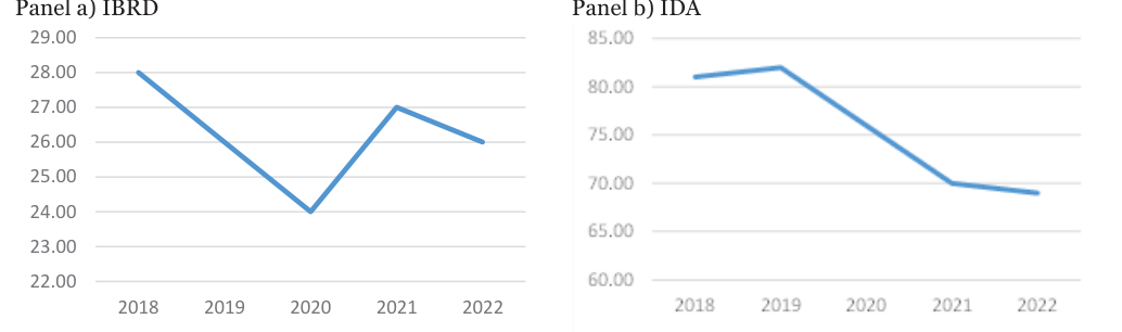
Note: Units are percent. The source of is S&P (2022d).
2.4 Key internal risk indicators
Both IBRD and IDA employ key risk indicators as central components of their capital adequacy policies and lending decisions. In the case of IBRD, the indicator in question is the institution’s Equity-to-Loans (E/L) ratio. 3 As part of IBRD’s Strategic Capital Adequacy framework, a floor level for the E/L ratio is periodically calibrated. The bank manages its balance sheet to ensure that the ratio remains above the floor level.
In the past, IBRD operated with a minimum threshold E/L ratio of 23%. In 2014, the target floor was reduced to 20%. This was justified by the institution on the basis that the credit quality of its portfolio had improved since 2008. Recently, IBRD has proposed a reduction in the floor to 19%. The institution has said this would be consistent with increased risk appetite by its shareholders (see World Bank (2023a)).
Figure 2.4 Panel a) shows the time path of the IBRD’s E/L from 2018 to 2022. The ratio has been stable even during the Covid 19 crisis and has consistently exceeded the policy minimum of 20%.
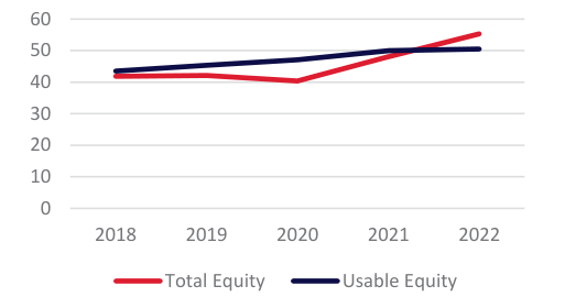
The numerator of the E/L ratio employed by IBRD is based on the institution’s own definition of ‘Usable Equity’. This aggregate differs from the Total Equity quantity provided in the institution’s financial statements. The latter Total Equity closely resembles what the ratings agencies employ in their rating evaluations (although there are some minor differences).
Figure 2.5 compares the paths of Total Equity and Usable Equity in recent years. The two variables can differ quite significantly. Usable Equity appears more stable. Total Equity declines in 2020 and subsequently rises rapidly. Usable Equity exhibits moderate and steady growth before remaining flat in 2022.[4]
The key financial indicator used by IDA in its balance sheet management is Deployable Strategic Capital (DSC). DSC is defined as the available capital to support future commitments, over and above the current portfolio. DSC is calculated as the difference of Total Resources Available (TRA) and Total Resources Required (TRR), plus a Conservation Buffer (CB). IDA has set the minimum allowable DSC to be 0%.
The TRA is the sum of IDA’s equity and accumulated provision for loan losses and other exposures. The TRR is the minimum capital required to cover expected and unexpected losses subjected to stress scenario as per the solvency-based capital adequacy model. In broad terms, the TRA is, therefore, the Capital Adequacy Ratio (capital available divided by capital requirement) minus 1 and minus a buffer. Here, the Unexpected Loss is calculated using risk models and, hence, the approach may be characterised as one based on Economic Capital. model. The CB is 10% of TRA. Note that IDA’s TRR includes, in addition to classic EC, a loan subsidy valuation adjustment that we discuss further in Section 2.8 below.
The DSC has declined in the past two years from 35.8% in 2020 to 26.4% in 2022, a fall of 9.4% percentage points. The fall in 2022 was essential due to the higher TRR (higher capital requirements to support conditional development grants). The ratio, nevertheless, remains safely above the policy threshold of 0% (see Panel b) of Figure 2.4.
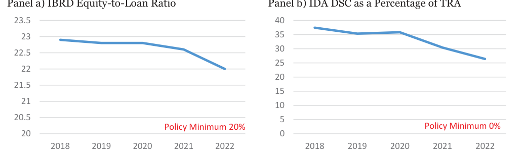
Note: Units are percent. The source for Panel a) is IBRD (2022) and IBRD (2021). The source for Panel b) is IDA (2022) and IDA (2021).
Note: Units are USD billion. The source for Panel a) is IBRD (2022), IBRD (2020) and IBRD & IDA (2018).
2.5 Portfolio composition
The International Bank for Reconstruction and Development (IBRD) and the International Development Association (IDA) provide data on their sovereign exposures in their financial statements. These are based on information for the fiscal year end in June of each year. The exposures analysed here are those contained in the latest annual report dated June 2022.
We calculate the total exposure at default (EAD), applying a Credit Conversion Factor (CCF) of 50% to the face value of undisbursed loans, i.e., ܧܣܦ=ܱݑݐݏݐܽ݊݀݅݊݃ܮܽ݊ݏ+ͷͲΨ ×ܷ݊݀݅ݏܾݑݎݏ݁݀ܮܽ݊ݏ. The total EAD for each institution is displayed in Table 2.1. The exposure amounts of the two institutions are broadly comparable although IDA has a somewhat lower volume of outstanding loans.
The loans of IBRD and IDA have very different geographical distributions. The IDA lends to Low-Income Countries (LICs) whereas the IBRD mainly lends to Medium- and High-Income Countries (MICs and HICs).[5] 133 unique countries have loans from either IBRD or IDA. Table 2.2 shows the regional distributions of the two institutions’ loan books. Just 14% of IBRD loans by EAD are to African countries whereas the comparable percentage for IDA is 51%. IDA has almost no exposure to Europe and Middle East or to Latin America.
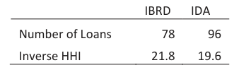
The effective number of exposures in a portfolio may be measured (approximately) using the inverse of the Herfindahl-Hirschman index[6] (HHI). If they are of equal size, the inverse index equals the number of exposures and otherwise may be thought of as an approximate measure of effective exposure number. Hence, the inverse HHI is often regarded as the notional “equivalent equal-sized exposure number”.
For IBRD’s sovereign loan portfolio, the inverse HHI is 21.8, whereas it is 19.6 for the sovereign loan portfolio of IDA (see Table 2.3). Hence, one may regard the IBRD and IDA’s portfolios are having concentration comparable to portfolios with 22 and 20 equal-sized exposures.
| KƵƚƐƚĂŶĚŝŶŐ >ŽĂŶƐ | ϮϮϵ͕ϯϰϰ | ϭϳϳ͕ϳϮϭ |
|---|---|---|
| hŶĚŝƐďƵƌƐĞĚ >ŽĂŶƐ | ϳϰ͕ϱϮϯ | ϳϭ͕ϯϲϱ |
| dŽƚĂů | Ϯϲϲ͕ϲϬϲ | Ϯϭϯ͕ϰϬϰ |
Note: The amounts are in millions of USD. CCF of 50% is applied to the undisbursed loans to calculate EAD.
| ZĞŐŝŽŶ | ||||||||
|---|---|---|---|---|---|---|---|---|
| ŽƵŶƚ | ŽƵŶƚ ;йͿ | ;йͿ | ŽƵŶƚ | ŽƵŶƚ ;йͿ | ;йͿ | |||
| ĨƌŝĐĂ | ϭϳ | ϮϮй | ϯϳ͕ϴϮϮ | ϭϰй | ϰϱ | ϰϳй | ϭϬϴ͕ϭϱϴ | ϱϭй |
| ƐŝĂ | ϭϴ | Ϯϯй | ϵϲ͕ϲϬϱ | ϯϲй | Ϯϴ | Ϯϵй | ϵϲ͕ϭϬϲ | ϰϱй |
| ƵƌŽƉĞ ĂŶĚ DŝĚĚůĞ ĂƐƚ | ϭϵ | Ϯϰй | ϱϭ͕ϵϵϯ | ϮϬй | ϭϯ | ϭϰй | ϰ͕ϵϴϵ | Ϯй |
| >ĂƚŝŶ ŵĞƌŝĐĂ | Ϯϰ | ϯϭй | ϴϬ͕ϭϴϳ | ϯϬй | ϭϬ | ϭϬй | ϰ͕ϭϱϭ | Ϯй |
| dŽƚĂů ĐŽƵŶƚƌŝĞƐ | ϳϴ | ϭϬϬй | Ϯϲϲ͕ϲϬϲ | ϭϬϬй | ϵϲ | ϭϬϬй | Ϯϭϯ͕ϰϬϰ | ϭϬϬй |
2.6 Statutory and Country Limits
IBRD Articles of Agreement define a Statutory Lending Limit (SLL) which constrains the scale of the institution’s total lending. Article 3 (Section 3) of the Articles (see IBRD (2012)) states that: “The total amount outstanding of guarantees, participations in loans and direct loans made by the Bank shall not be increased at any time, if by such increase the total would exceed one hundred percent of the unimpaired subscribed capital, reserves and surplus of the Bank.” Hence, the SLL equals the sum of unimpaired subscribed capital, reserves and surplus of IBRD. In contrast, IDA’s Articles of Agreement do not specify a Statutory Lending Limits (see IDA (1960)).
In planning its future lending commitments, IBRD makes use of a Sustainable Annual Lending Limit (SALL). The SALL equals the maximum annual commitment level sustainable in real terms for 10 years based on Capital Adequacy Framework and SLL. The SALL is required by the Financial Sustainability Framework (FSF) for all sustainable lending activities and implements an additional buffer to respond to a crisis. The adjusted SALL (SALL-Adj) for the crisis buffer is the upper bound for regular lending.
In Fiscal Year 2022, the SALL-Adj was $28bn. This has been increased to $36.5bn for Fiscal Year 2023 and it includes an additional board-approved crisis buffer of $5bn and a carryover of unutilised crisis buffer of $4.5bn from Fiscal Year 2022.
The SLL also serves as the basis for a set of country limits within which the IBRD operates. Specifically, IBRD limits exposure[7] to a single country to the lower barrier of two quantities: the Equitable Access Limit (EAL) and the Single Borrower Limit (SBL).
The EAL is 10% of the SLL. In June 2022 SLL was $339bn thus EAL is $34bn. The SBL is the maximum exposure for the most creditworthy and largest borrowing country in terms of population and economic size. The amount is decided by the IBRD based on the impact of SBL on overall portfolio risk relative to equity.
On SBLs, IBRD operates a dual system in that the SBL amount depends on whether the country’s income exceeds the Graduation Discussion Income (GDI) or not.[8] For countries with income above the GDI, the SBL is lower. In Fiscal Year 2022, the SBL was $21.2bn for highly creditworthy countries above the GDI and $24.9 for the highly creditworthy countries below the GDI.[9][10]
The EAL exceeds the SBL by $10bn, so the SBL is the primary constraint for the IBRD. This makes it more difficult for the IBRD to boost lending to highly creditworthy sovereigns, potentially inducing it to lend more to countries with lower ratings.
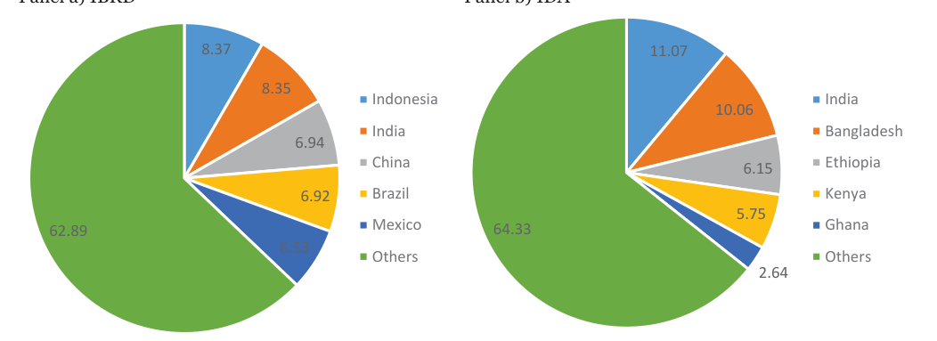
IDA also operates Single Borrower Limits (SBLs) to reduce portfolio concentration. To determine SBL, IDA relies on Basel maximum exposure limit which constrains exposure to be less than 25% of equity. For Fiscal Year 2023, the IDA SBL is $45bn (25% of $178.7bn equity as measured at end June 2022). In Fiscal Year 2022, 40% of net outstanding IBRD loans were concentrated in 5 countries (see Panel a) of Figure 2.6). IDA exhibited a similar degree of loan concentration in that around 40% of total outstanding loans were to the top 5 countries.
IBRD reports that four countries had binding SBL limits in Fiscal Year 2022. Two of these were above the GDI threshold and two below. No IDA borrowing countries had binding SBL limits in Fiscal Year 2022. The exposure to the highest borrowing country, India, is less than half of the SBL. Thus, SBLs do not currently constrain IDA lending decisions.
Note: The data for Panel a) is based on Total Outstanding Loans as of June 30, 2022, from IBRD (2022). The data for Panel b) is based on Total Outstanding Loans as of June 30, 2022 from IDA (2022).
2.7 Ratings distributions
This section examines credit ratings of the individual countries that borrow from IBRD and IDA. In this, we rely on ratings from the three global agencies, Standard & Poor’s, Moody’s, and Fitch. However, some countries that borrow from the institutions are not rated by these agencies. To infer ratings for these latter countries, we rely on the ratings provided by the Organisation for Economic Co-operation and Development (OECD). OECD ratings are on a different scale from that employed by the major agencies. So, we convert the OECD ratings to the latter scale using a mapping inferred from a regression of the Standard & Poor’s ratings on OECD ratings.
We create a consolidated set of ratings by using in order of preference and depending on availability Standard & Poor’s, Moody’s, Fitch and transformed OECD ratings. This provides ratings for most countries. Table 2.4 shows the rating coverage of the consolidated data. The coverage in terms of exposure amount is almost complete. Countries that borrow from IDA are less likely to have agency ratings than those that borrow from IBRD.
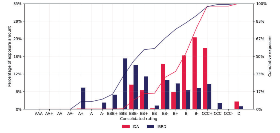
Figure 2.7 displays the distribution of ratings. More than half of IBRD’s exposure amount is from countries with ratings higher than or equal to BB+. On the other hand, IDA exposures have lower ratings. Half of them being in ratings higher than or equal to B. In IDA’s portfolio, there are many countries that do not have an agency rating and we rely on the OECD rating. In most of those cases, the ratings are CCC+, as we can observe in Figure 2.7, this is the rating of a fifth of the portfolio exposure measured in terms of exposure value.
Three countries in IBRD’s portfolio are regarded as in default by the rating agencies: Lebanon, Sri Lanka and Suriname. In IDA’s portfolio, the agencies similarly regard three countries as being in default: Lebanon, Sri Lanka and Zambia. These countries are not in default to the MDBs according to the MDBs’ arrears data, however. We map all ratings below CCC+ (including defaults) to a consolidated rating of “Cs” for use in subsequent sections. Following this approach, the weighted average rating of IBRD’s portfolio is BB+/BB and the weighted average rating of IDA’s portfolio is B+/B.
| D | й >ŽĂŶƐ ĐŽǀĞƌĞĚ | й >ŽĂŶƐ ĐŽǀĞƌĞĚ | й >ŽĂŶƐ ĐŽǀĞƌĞĚ ^ΘW Žƌ DŽŽĚLJƐ Žƌ | й >ŽĂŶƐ ĐŽǀĞƌĞĚ ^ΘW Žƌ DŽŽĚLJƐ Žƌ | й ĂƐĞƐ ĐŽǀĞƌĞĚ | й ĂƐĞƐ ĐŽǀĞƌĞĚ | й ĂƐĞƐ ĐŽǀĞƌĞĚ ^ΘW Žƌ DŽŽĚLJƐ Žƌ | й ĂƐĞƐ ĐŽǀĞƌĞĚ ^ΘW Žƌ DŽŽĚLJƐ Žƌ |
|---|---|---|---|---|---|---|---|---|
| ^ΘW | ^ΘW Žƌ DŽŽĚLJƐ | &ŝƚĐŚ | &ŝƚĐŚ Žƌ K | ^ΘW | ^ΘW Žƌ DŽŽĚLJƐ | &ŝƚĐŚ | &ŝƚĐŚ Žƌ K | |
| / Z | ϵϲ͘ϰϲй | ϵϴ͘ϯϴй | ϵϴ͘ϯϴй | ϵϵ͘ϵϲй | ϳϲ͘ϵϮй | ϴϬ͘ϳϳй | ϴϬ͘ϳϳй | ϵϲ͘ϭϱй |
| / | ϳϮ͘Ϯϳй | ϳϮ͘Ϯϳй | ϳϮ͘Ϯϳй | ϵϵ͘ϭϰй | ϰϳ͘ϭϮй | ϰϴ͘Ϭϴй | ϰϴ͘Ϭϴй | ϴϴ͘ϰϲй |
2.8 Valuing IDA’s interest rate subsidies
As explained in the introduction, IDA’s loans contain substantial subsidy elements in that they carry, in many cases, an interest rate of zero. Such interest rates remunerate neither time preference nor the credit risk associated with possible failures to repay by the institution’s sovereign borrowers. The size of the credit risk component is undoubtedly reduced by the de facto seniority that IDA enjoys, commonly referred to as Preferred Creditor Treatment (PCT). But taken together, the fact that lending rates omit both a default free interest rate component and a credit spread means that the value of these loans is substantially less than their par value.
IDA’s accounts are, of course, prepared on a going concern basis. The value of IDA’s loans may, therefore, be recorded at par on the basis that the loans are financed using the institution’s own equity. Implicitly, this argument depends on the fact that the equity is not expected to generate dividends. However, if one wishes to evaluate IDA’s assets on a non-going-concern basis, as may be appropriate for credit analysis, one may wish to record loans values less than par.[11] The three major rating agencies do not adjust IDA’s loan values (and hence equity) for the institution’s loan subsidies. However, IDA chooses to take a conservative approach in its internal capital adequacy analysis in that it adjusts up its Total Required Resources to include the value of loan subsidies. In our analysis below, we shall instead reduce equity resources by the amount of loan subsidies, but the adjustment may be regarded as equivalently conservative (and more conservative than the approach of the rating agencies).
In IDA’s balance sheet, loans are recorded at par even though they are issued on concessional or subsidised terms. To allow for this, in its internal risk management, IDA adds an estimate of the subsidy value to the more conventional ‘Economic Capital components’ of its TRR. IDA (2022) briefly explains this, stating: “Within the TRR there is also a capital allowance to reflect losses that result from valuing IDA’s concessional loan portfolio in present value terms using market interest rates.”
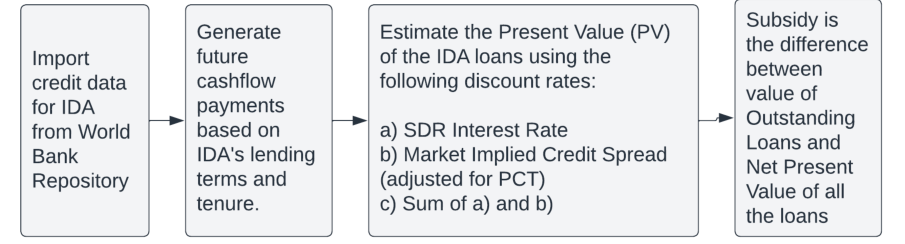
Below, we present the results of our own valuation of the subsidy component in the value of IDA’s loan book. The valuation exercise we perform starts from granular data on individual IDA loans provided by the World Bank Repository (2023). To obtain results consistent with our other calculations, we include all loans contained in IDA’s loan portfolio on 30th June 2022.
The approach followed in estimating the subsidy element is explained in Figure 2.8. From the repository data, we construct cashflow payment profiles loan-by-loan using the loan terms recorded on the WBG website. We discount these cashflows to end-June 2022 using SDR interest rate term structures to which we add credit spreads. The credit spreads are derived from market sovereign credit spreads but adjusted for PCT.
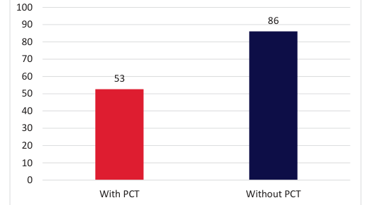
We compute the subsidy element in the value of the loan book to be $52.58 bn when SDR interest rates and PCT-adjusted credit spreads are included in the discount factors. This compares to the value of IDA’s concessional lending of $171.90 bn. (Including non-concessional lending, the loan book value recorded in the accounts is $178.04 bn.) When credit spreads are employed that do not adjust for PCT, the subsidy element rises to $86.09 bn (see Figure 2.9).
One may split the subsidy element down by loan types as shown in Panel a) of Figure 2.10. The largest fraction of IDA’s outstanding loans is provided under ‘Small Economy’ terms. This category contributes 46% of total subsidy. Panel b) of Figure 2.10 shows how the subsidy element in the end-June 2022 portfolio value is distributed across individual calendar year loan issuance. The peak contribution to the total subsidy is attributable to loans originated between 2011 and 2020. The average subsidy per year during 2012-2020 (both inclusive) is $3.07bn, compared to the lifetime average per year (i.e., 1972-2022) of $1.03bn. These calculations show the loan vintages in the end-June 2022 portfolio that contributed most to the total subsidy element. Since loans in earlier periods have fully or partly matured, one cannot deduce from this whether subsidisation has increased.
Note: The unit of Y-axis is USD billion.
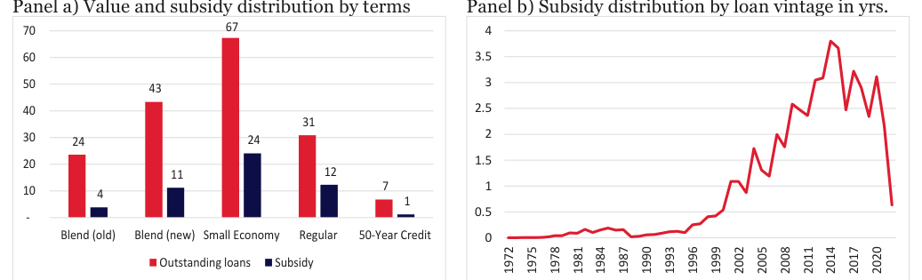
Note: ‘Blend (old)’ also includes ‘hard term’ loans which Note: The data is up to 30 June 2022. Units on the vertical axis were discontinued in 2017. Units on the vertical axis are in are USD billions. The subsidy is adjusted for PCT. The vintages USD billions. The subsidy is adjusted for PCT. are defined by calendar years.
3. Rating Analysis of IBRD and IDA
3.1 MDB ratings
This section analyses the ratings of IBRD and IDA provided by the three global rating agencies, Standard & Poor’s, Moody’s, and Fitch. We consider how these ratings would evolve if the two MDBs’ expanded their Development Related Assets (DRAs) and Treasury Assets, financed by additional borrowing without changes in their Total Equity or Callable Capital.
To understand the agencies’ ratings, we replicate the process that the agencies go through in determining the components of their respective scorecards. The approach takes as inputs granular data on the assets, liabilities, and financial variables of the MDB in question. IBRD and IDA publish some of this data in their annual reports. Some data are missing, however, for example the maturities of individual loans and Treasury assets.
So, we are obliged to make reasonable assumptions based on the aggregate information provided. Again, the obliged to make reasonable as agencies’ reports on MDB ratings assessments provide partial information on intermediate findings. Where reports on MDB ratings assess information is available, we match the values provided by the agencies and otherwise, we make assumptions. on is available, we match the v
3.2 Data collectionData collection
We employ publicly available data contained in financial statements posted on the World Bank Group website oy publicly available data conta (see IBRD(2022) and IDA (2022)). We utilize the most recent financial statements available, dated end June D(2022) and IDA (2022)). We
2022. The financial statements include Development Related Assets (DRAs) broken down by country with e fif nancial statements include D information on disbursed and undisbursed amounts. Information is available for equity (segregated by callable on on disbursed and undisburs and subscribed capital) for each member country.
In addition to data from the financial statements, we collect ratings for the sovereigns represented either in the portfolio or in the shareholders list. The ratings data coincide with the date of the financial statements, providing a snapshot of the IBRD and IDA portfolio at end June 2022.
To replicate the Standard & Poor’s RAC calculation requires a correlation matrix for individual countries risk factors. To estimate a correlation matrix, we employ log changes in MSCI equity indices for countries.[12] Detail s of the MSCI indices employed are provided in the appendix.
Some other information is needed to populate the data required by the rating application. In particular, the rating agencies make qualitative judgments. In the case of Moody’s these are mostly stated explicitly as questions in the methodology document. The possible answers are often binary or envisage several possible answers (e.g., the MDB is deemed to be high, medium, or low in some respect).
The Moody’s methodology, in most cases, provides guidance on how much intermediate results should be adjusted by one or more plus or minus categories following answers to the questions. The other agencies (especially Fitch) make use of judgmental elements in a less transparent way. In these cases, our approach is to express the judgmental adjustment in the form of a clear question with a categorical answer that we map into a set of adjustments in intermediate results. This technique may be regarded, ion very general terms, as following the approach of Moody’s in which qualitative questions determine which branch to select in a well-defined decision-tree.
One area in which it is necessary to make assumptions is the quantitative liquidity indicators the agencies employ. This is the case because information is lacking on the maturity of the two institutions’ assets and liabilities. Starting from the aggregate information on maturity that the institutions provide in their financial ggreg statements, we infer a reasonable set of maturities for country loan exposures. In Box 3.1, we discuss issues able s specific to each of the rating agencies. Additional agency-specific data issues are discussed in Appendix 1.agenci
3.3 Current and possible future ratingsble fu
As mentioned in the previous section, we take the data from 2022 as a starting point for the scenarios that we sectc io analysis in this exercise. In this, we employ the latest rating reports as available in March 2023 (for IBRD see his, we
a) and S&P (2023a), Moody’s (2023a) and Fitch (2023); for IDA see IDA S&P (2023b) and Moody’s (2023b)). IBRD and IDA have the highest rating for the three rating agencies (AAA for S&P and Fitch and Aaa for Moody’s). ng for
The rating agencies specify in their reports, which factors are most likely to lead to a change in rating. In the their case of IBRD, Standard & Poor’s suggests that the two main reasons there could be a downgrade would be if there were more aggressive financial policies and if the members were to stop treating IBRD as a preferred creditor. The agency emphasises the fact that IBRD has substantial eligible callable capital that would keep the RAC ratio above 23%.
Moody’s emphasise capital adequacy as a driver of a potential downgrade. Moody’s capital adequacy is driven by the leverage ratio. This would certainly increase DRAs were to grow substantially. Another factor mentioned by Moody’s is that could potentially lead to a downgrade is loss of the shareholder support that the IBRD currently enjoys.
Fitch identifies the Solvency Factor as a potential source of a downgrade. The Fitch Solvency Factor depends on the two sub-factors Capitalisation and Risks. Capitalisation is based on three ratios, the Equity to Assets ratio, the ratio of Usable Capital to RWA and the Return on Equity (ROE). As we will see below, the Capitalisation Factor worsens if DRAs grow. The Risk element of the Solvency Factor could worsen due to greater concentration or a weakening of the credit quality of the portfolio.
In the case of IDA, Standard & Poor’s state that their rating has a stable outlook and very low chance of suffering a downgrade. The downside scenario in which the IDA rating might be downgraded is if the RAC ratio fell below 23%. (IDA does not have Callable Capital which could provide uplift.) Another possible downgrade scenario is that liquidity deteriorate.
For IDA, the factors that could lead to a downgrade in the Moody’s rating are the deterioration of IDA’s capital adequacy through a default of a large borrower or if one of the key donor countries significantly reduced its contributions. However, Moody’s affirms that IDA’s credit metrics are very likely to remain stable if there is an expansion in leverage. This will be tested in the analysis in the next section.
| ZĂƚŝŶŐ ƌĞƐƵůƚƐ ͬ zĞĂƌ | ϮϬϮϮ | ϮϬϮϯ | ZĂƚŝŶŐ ƌĞƐƵůƚƐ ͬ zĞĂƌ | ϮϬϮϭ | ϮϬϮϮ | ||
|---|---|---|---|---|---|---|---|
| / Z | / Z | ||||||
| /ƐƐƵĞƌ ƌĞĚŝƚ ZĂƚŝŶŐ Ͳ &ŽƌĞŝŐŶ ƵƌƌĞŶĐLJ | ͬ^ƚĂďůĞͬ Ͳϭн | ͬ^ƚĂďůĞͬ Ͳϭн | ^ĐŽƌĞĐĂƌĚͲ/ŶĚŝĐĂƚĞĚ KƵƚĐŽŵĞ ZĂŶŐĞ | ĂĂͲ ĂϮ | ĂĂͲ ĂϮ | ||
| ŶƚĞƌƉƌŝƐĞ ƌŝƐŬ ƉƌŽĨŝůĞ | džƚƌĞŵĞůLJ ^ƚƌŽŶŐ | džƚƌĞŵĞůLJ ^ƚƌŽŶŐ | ĚũƵƐƚĞĚ ŝŶƚƌŝŶƐŝĐ ĨŝŶĂŶĐŝĂů ƐƚƌĞŶŐƚŚ | ĂĂϭ | ĂĂϭ | ||
| WŽůŝĐLJ ŝŵƉŽƌƚĂŶĐĞ 'ŽǀĞƌŶĂŶĐĞ ĂŶĚ ŵĂŶĂŐĞŵĞŶƚ ĞdžƉĞƌƚŝƐĞ &ŝŶĂŶĐŝĂů ƌŝƐŬ ƉƌŽĨŝůĞ | sĞƌLJ ^ƚƌŽŶŐ ^ƚƌŽŶŐ džƚƌĞŵĞůLJ ^ƚƌŽŶŐ | sĞƌLJ ^ƚƌŽŶŐ ^ƚƌŽŶŐ džƚƌĞŵĞůLJ ^ƚƌŽŶŐ | ^ƚƌĞŶŐƚŚ ŽĨ ŵĞŵďĞƌ ƐƵƉƉŽƌƚ WƌĞůŝŵŝŶĂƌLJ ŝŶƚƌŝŶƐŝĐ ĨŝŶĂŶĐŝĂů ƐƚƌĞŶŐƚŚ YƵĂůŝƚĂƚŝǀĞ ĂĚũƵƐƚŵĞŶƚƐ | sĞƌLJ ,ŝŐŚ ĂĂϮ нϭ | sĞƌLJ ,ŝŐŚ ĂĂϮ нϭ | ||
| ĂƉŝƚĂů ĂĚĞƋƵĂĐLJ Z ZĂƚŝŽ &ƵŶĚŝŶŐ ĂŶĚ ůŝƋƵŝĚŝƚLJ / | džƚƌĞŵĞůLJ ^ƚƌŽŶŐ Ϯϳ͘Ϯй ^ƚƌŽŶŐ | džƚƌĞŵĞůLJ ^ƚƌŽŶŐ Ϯϱ͘ϵй ^ƚƌŽŶŐ | ĂƉŝƚĂů ĂĚĞƋƵĂĐLJ >ŝƋƵŝĚŝƚLJ ĂŶĚ ĨƵŶĚŝŶŐ / | Ăϭ ĂĂϭ | Ăϭ ĂĂϯ | ||
| /ƐƐƵĞƌ ƌĞĚŝƚ ZĂƚŝŶŐ Ͳ &ŽƌĞŝŐŶ ƵƌƌĞŶĐLJ | ͬ^ƚĂďůĞͬ Ͳϭн | ͬ^ƚĂďůĞͬ Ͳϭн | ^ĐŽƌĞĐĂƌĚͲ/ŶĚŝĐĂƚĞĚ KƵƚĐŽŵĞ ZĂŶŐĞ | ĂĂͲ ĂϮ | ĂĂͲ ĂϮ | ||
| ŶƚĞƌƉƌŝƐĞ ƌŝƐŬ ƉƌŽĨŝůĞ | džƚƌĞŵĞůLJ ^ƚƌŽŶŐ | džƚƌĞŵĞůLJ ^ƚƌŽŶŐ | ĚũƵƐƚĞĚ ŝŶƚƌŝŶƐŝĐ ĨŝŶĂŶĐŝĂů ƐƚƌĞŶŐƚŚ | ĂĂϭ | ĂĂĂ | ||
| WŽůŝĐLJ ŝŵƉŽƌƚĂŶĐĞ | sĞƌLJ ^ƚƌŽŶŐ | sĞƌLJ ^ƚƌŽŶŐ | ^ƚƌĞŶŐƚŚ ŽĨ ŵĞŵďĞƌ ƐƵƉƉŽƌƚ | ,ŝŐŚ | ,ŝŐŚ | ||
| 'ŽǀĞƌŶĂŶĐĞ ĂŶĚ ŵĂŶĂŐĞŵĞŶƚ ĞdžƉĞƌƚŝƐĞ | ^ƚƌŽŶŐ | ^ƚƌŽŶŐ | WƌĞůŝŵŝŶĂƌLJ ŝŶƚƌŝŶƐŝĐ ĨŝŶĂŶĐŝĂů ƐƚƌĞŶŐƚŚ | ĂĂϮ | ĂĂϭ | ||
| &ŝŶĂŶĐŝĂů ƌŝƐŬ ƉƌŽĨŝůĞ | džƚƌĞŵĞůLJ ^ƚƌŽŶŐ | džƚƌĞŵĞůLJ ^ƚƌŽŶŐ | YƵĂůŝƚĂƚŝǀĞ ĂĚũƵƐƚŵĞŶƚƐ | нϭ | нϭ | ||
| ĂƉŝƚĂů ĂĚĞƋƵĂĐLJ | džƚƌĞŵĞůLJ ^ƚƌŽŶŐ | džƚƌĞŵĞůLJ ^ƚƌŽŶŐ | ĂƉŝƚĂů ĂĚĞƋƵĂĐLJ | Ăϭ | ĂĂϯ | ||
| Z ZĂƚŝŽ | ϳϬ͘Ϭй | ϲϴ͘ϴй | >ŝƋƵŝĚŝƚLJ ĂŶĚ ĨƵŶĚŝŶŐ | ĂĂĂ | ĂĂĂ | ||
| &ƵŶĚŝŶŐ ĂŶĚ ůŝƋƵŝĚŝƚLJ | ^ƚƌŽŶŐ | ^ƚƌŽŶŐ | |||||
| Panel c) Fitch | |||||||
| ZĂƚŝŶŐ ƌĞƐƵůƚƐ ͬ zĞĂƌ | ϮϬϮϭ | ϮϬϮϮ | |||||
| / Z | |||||||
| ĂƉŝƚĂůŝnjĂƚŝŽŶ | ^ƚƌŽŶŐ | ^ƚƌŽŶŐ | |||||
| ZŝƐŬƐ | >Žǁ | ƌŝƐŬ | >Žǁ ƌŝƐŬ | ||||
| ^ŽůǀĞŶĐLJ | ĂĂ | ĂĂ | |||||
| >ŝƋƵŝĚŝƚLJ | ĂĂĂ | ĂĂĂ | |||||
| ƵƐŝŶĞƐƐ ĞŶǀŝƌŽŶŵĞŶƚ | >Žǁ | ƌŝƐŬ | >Žǁ ƌŝƐŬ | ||||
| džƚƌĂŽƌĚŝŶĂƌLJ ^ƵƉƉŽƌƚ | ĂĂͲ | ĂĂͲ | |||||
| ZĂƚŝŶŐ |
Note: IDA is not rated by Fitch.
3.4 Lending growth scenarios
We begin by calibrating a data set of granular data for each of the two MDBs so that the institutions’ ratings (and all published intermediate indicators) match those published by the rating agencies in their latest rating assessment reports.
We then design a set of scenarios in which loans increase in proportion to the current portfolio. In our software, we define 300 scenarios in which the loan portfolio grows by 1% increments. For each percentage we calculated the rating and its intermediate elements and components. To avoid deterioration in the liquidity metrics that the agencies use as inputs to their rating evaluations, we assume that Treasury assets grow in proportion to the increase in loans. Borrowing increases to finance the higher DRA and Treasury assets while equity is assumed to remain constant.
In addition to the changes in DRA and Treasury assets just described, we expect that the agencies would change some qualitative ratings factors as the institutions adopted the new policy of loan portfolio growth. We represent these qualitative factors as responses to questions. For each agency, we adopted assumptions about how the answers to the questions would change as the portfolio grows[13]. The changes are displayed in Table 3.2, Table 3.5, and Table 3.8. For a portfolio change less than 50%, we assume that the qualitative factors would not change so the answers to the questions would remain as they were. For lending increases from 50% to 150%, we assume a particular set of changes in the answers. For increase greater than 150%, we assume that the answers change even more.
The purpose of examining different scenarios is to identify the thresholds at which the ratings change. As we increase the loans the capital adequacy indicators face more stress until they finally lead to a downgrade of the ratings. In later subsections, we discuss the results for each individual rating agency. In each case, these follow the same structure.
Take as an example the right-hand columns is downgraded. For example, take the first value in the left-hand column in Table 3.3, i.e., 75. This indicates that, the DRAs and Treasury assets may increase up to 75% until a downgrade occurs in “Capital Adequacy.” When the downgrade in a metric implies a downgrade in the overall final rating it is highlighted in red.
3.5 Standard & Poor’s findings
As the scale of lending increases, the Standard & Poor’s ratings for IBRD and IDA tend to deteriorate because of two different factors: (a) Capital Adequacy and (b) Liquidity and Funding. Capital Adequacy is initially evaluated based on the RAC ratio and is then notched (up or down) depending on loan performance and additional qualitative elements of the RAC ratio. The Liquidity and Funding factor is calculated using the funding rating for 6 and 12-month horizons and the gap ratio.
The liquidity ratio would deteriorate very substantially if an MDB increased DRAs only. In this case, borrowings would grow to finance the additional and outflows would exceed inflows.[14] To offset a deterioration in liquidity metrics, we assume that Treasury assets grow in proportion to the DRA. As we can see in Table 3.3 and Table 3.4 the liquidity ratio for 12 months nevertheless deteriorates somewhat as we increase the DRAs and Treasury assets.
The capital adequacy and liquidity and funding factors are combined into the financial risk profile. Subsequently the financial risk profile is combined with the enterprise risk profile, the enterprise risk profiles is not affected through this exercise, for both the IBRD and IDA the enterprise risk profiles are “extremely strong.”
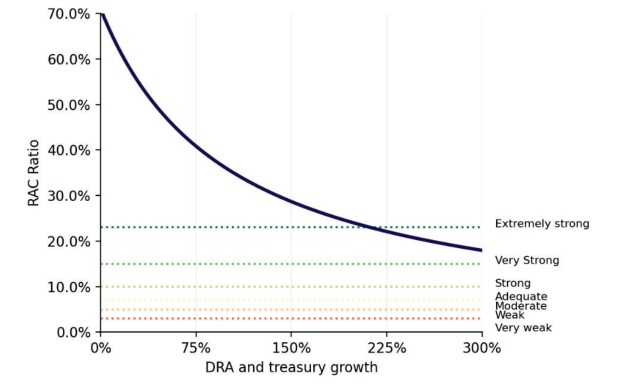
As we can see in Table 3.3 and Table 3.4, the RAC ratio falls as the DRA and Treasury assets grow. The capital adequacy of the IBRD changes from its initial evaluation of “Extremely strong” to “Moderate”. The points at which the values change appear in the left-hand column of the tables. For increases up to 150%, the decline in the RAC ratio is not enough to generate a downgrade in capital adequacy. Instead, the worsening of the qualitative question which is assumed to happen at that level of portfolio expansion is what leads to the capital adequacy downgrade.
An overall rating downgrade for IBRD occurs after the DRAs and Treasury assets increase by 164%. In this case, capital adequacy goes from “Adequate” to “Moderate” which leads to a deterioration in the Stand-Alone Credit Profile (SACP) to a+. The enhanced financial risk profile that results from allowing for the Callable Capital provides an uplift that results in the final rating being AA+.
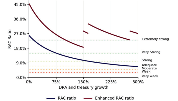
Note: The enhanced RAC ratio includes the eligible callable capital in the calculation, the jumps in the enhanced RAC ratio are produced by the fact that the SACP rating deteriorates and therefore more callable capital becomes eligible. Eligible callable capital is all the callable capital from shareholders that have the same or higher rating as the SACP.
Note: IDA has no callable capital so there is no enhance RAC ratio calculation.
| &ĂĐƚŽƌ | ^ƵďͲĨĂĐƚŽƌ | YƵĞƐƚŝŽŶ | KƌŝŐŝŶĂů ƌĞƐƉŽŶƐĞ | ĨƚĞƌ ϱϬй ƉŽƌƚĨŽůŝŽ | ĨƚĞƌ ϭϱϬй ƉŽƌƚĨŽůŝŽ |
|---|---|---|---|---|---|
| ŐƌŽǁƚŚ | ŐƌŽǁƚŚ | ||||
| ,ĂƐ ƚŚĞ ĂŶŬ ĂĐŚŝĞǀĞĚ ŵŽƌĞ ĂŐŐƌĞƐƐŝǀĞ ƌĞĐĞŶƚ | |||||
| ŐŐƌĞƐƐŝǀĞ ƌĞĐĞŶƚ | ŽƌŐĂŶŝĐ ŐƌŽǁƚŚ ĂŶĚ ŵŽƌĞ ƐŝŐŶŝĨŝĐĂŶƚ ƉƌŽƐƉĞĐƚƐ ĨŽƌ | zĞƐ | |||
| ŽƌŐĂŶŝĐ ŐƌŽǁƚŚ | ĨƵƚƵƌĞ ŐƌŽǁƚŚ ƚŚĂŶ ŝŶ ƚŚĞ ƉĂƐƚ͕ ĐŽŵƉĂƌĞĚ ǁŝƚŚ | EŽ | |||
| ŽƚŚĞƌ D>/Ɛ ŝŶ ƐŝŵŝůĂƌ ƌĞŐŝŽŶƐ͍ | |||||
| ŽŵƉĂƌĞĚ ƚŽ ŽƚŚĞƌ D>/Ɛ͕ ĚŽĞƐ ƚŚĞ ĂŶŬ ďŽĂƐƚ | |||||
| >ŽĂŶ ƉĞƌĨŽƌŵĂŶĐĞ | ŽŶƐĞƌǀĂƚŝǀĞ ƌŝƐŬ | ƐƚƌŽŶŐĞƌ ĐŽŶƐĞƌǀĂƚŝǀĞ ƌŝƐŬ ƚŽůĞƌĂŶĐĞƐ ĂŶĚ | zĞƐ | ||
| ĂŶĚ ƌŝƐŬ | ƚŽůĞƌĂŶĐĞƐ | ƵŶĚĞƌǁƌŝƚŝŶŐ ƐƚĂŶĚĂƌĚƐ ĚƵƌŝŶŐ ƉĞƌŝŽĚƐ ŽĨ ŐƌŽǁƚŚ Žƌ ĐŚĂŶŐĞƐ ŝŶ ĞdžƉŽƐƵƌĞ ;ŶŽƚĂďůLJ ǁŚŝůĞ ĨƵůĨŝůůŝŶŐ ŝƚƐ | EŽ | ||
| ŵĂŶĂŐĞŵĞŶƚ | ĐŽƵŶƚĞƌĐLJĐůŝĐĂů ůĞŶĚŝŶŐ ƌŽůĞͿ͍ | ||||
| ŐŐƌĞƐƐŝǀĞ ƌŝƐŬ | ŽŵƉĂƌĞĚ ƚŽ ŽƚŚĞƌ D>/Ɛ͕ ĚŽĞƐ ƚŚĞ ĂŶŬ ĨŽůůŽǁ | EŽ | |||
| ƚŽůĞƌĂŶĐĞƐ | ŵŽƌĞ ĂŐŐƌĞƐƐŝǀĞ ƌŝƐŬ ƚŽůĞƌĂŶĐĞ ƉŽůŝĐŝĞƐ͍ | zĞƐ | |||
| tĞĂŬĞƌ ůŽĂŶ | ŽĞƐ ƚŚĞ ĂŶŬ ŚĂǀĞ ǁĞĂŬĞƌ ůŽĂŶ ĐŽŶĚŝƚŝŽŶĂůŝƚLJ | EŽ | |||
| ĐŽŶĚŝƚŝŽŶĂůŝƚLJ | ƌĞůĂƚŝǀĞ ƚŽ ƉĞĞƌƐ͍ | zĞƐ | |||
| >ŝƋƵŝĚŝƚLJ ƐƚĂƚƵƐ | tŚĂƚ ƚƌĞŶĚ ĚŽĞƐ ƚŚĞ ĂŶŬ ĞdžƉĞĐƚ ŝŶ ŝƚƐ ůŝƋƵŝĚŝƚLJ | ĞƚĞƌŝŽƌĂƚŝŶŐ | |||
| >ŝƋƵŝĚŝƚLJ | ƚƌĞŶĚ | ƐƚĂƚƵƐ͍ | ^ƚĂďůĞ |
| Z н dƌĞĂƐƵƌLJ | ϭϮ ŵŽŶƚŚ | >ŝƋƵŝĚŝƚLJ ĂŶĚ | &ŝŶĂŶĐŝĂů ZŝƐŬ | ŶƚĞƌƉƌŝƐĞ | ŶŚĂŶĐĞĚ ŶŚĂŶĐĞĚ &ŝŶĂŶĐŝĂů ŶŚĂŶĐĞĚ | /ŶĚŝĐĂƚŝǀĞ | ||||
|---|---|---|---|---|---|---|---|---|---|---|
| ŐƌŽǁƚŚ ;йͿ | Z ;йͿ | ůŝƋƵŝĚŝƚLJ | ĂƉŝƚĂů ĚĞƋƵĂĐLJ | &ƵŶĚŝŶŐ | WƌŽĨŝůĞ | ZŝƐŬ WƌŽĨŝůĞ | ^ W Z | ;йͿ ZŝƐŬ WƌŽĨŝůĞ ^ W | / Z | &ŝŶĂů / |
| Ϭ | Ϯϱ͘ϵϲ | ϮϬϰ͘Ϭϰ | džƚƌĞŵĞůLJ ƐƚƌŽŶŐ | džƚƌĞŵĞůLJ ƐƚƌŽŶŐ | ĂĂĂ | ϰϱ͘ϳ | ||||
| ϳϱ | ϭϰ͘ϵϵ | ϭϴϵ͘ϰϳ | sĞƌLJ ƐƚƌŽŶŐ | ^ƚƌŽŶŐ | sĞƌLJ ƐƚƌŽŶŐ | džƚƌĞŵĞůLJ | ĂĂн | Ϯϲ͘ϰ džƚƌĞŵĞůLJ ƐƚƌŽŶŐ ĂĂĂ | ||
| ϭϱϬ ϭϲϰ | ϭϬ͘ϱϰ ϵ͘ϵϴ | ϭϴϰ͘Ϯϴ ϭϴϯ͘ϲϲ | ^ƚƌŽŶŐ ĚĞƋƵĂƚĞ | ^ƚƌŽŶŐ ĚĞƋƵĂƚĞ | ƐƚƌŽŶŐ | ĂĂ ĂĂͲ | Ϯϴ͘ϱ ϯϮ͘ϵ | н | н | |
| Ϯϳϴ | ϲ͘ϵϵ | ϭϴϬ͘ϯϴ | DŽĚĞƌĂƚĞ | DŽĚĞƌĂƚĞ | Ă | Ϯϴ͘ϲ | Ͳ | Ͳ | ||
| Note: When | calculating | the | ICR we took | into | consideration that | IBRD | would | benefit from up to two notches of | uplift | from |
Note: When calculating the ICR we took into consideration that IBRD would benefit from up to two notches of uplift from callable capital. The number of notches is defined by assessing (1) Legal and administrative processes that ensure a capital call (2) Ability to make payments of additional capital, 3) Willingness to make payment when the capital is called and 4) Policy importance.
| Z н dƌĞĂƐƵƌLJ | ϭϮ ŵŽŶƚŚ | >ŝƋƵŝĚŝƚLJ ĂŶĚ | &ŝŶĂŶĐŝĂů ZŝƐŬ | ŶƚĞƌƉƌŝƐĞ | ŶŚĂŶĐĞĚ | ŶŚĂŶĐĞĚ &ŝŶĂŶĐŝĂů | ŶŚĂŶĐĞĚ | /ŶĚŝĐĂƚŝǀĞ | |||
|---|---|---|---|---|---|---|---|---|---|---|---|
| ŐƌŽǁƚŚ ;йͿ | Z ;йͿ | ĂƉŝƚĂů ĚĞƋƵĂĐLJ ůŝƋƵŝĚŝƚLJ | &ƵŶĚŝŶŐ | WƌŽĨŝůĞ | ZŝƐŬ WƌŽĨŝůĞ | ^ W | Z ;йͿ | ZŝƐŬ WƌŽĨŝůĞ | ^ WΎ | / Z | &ŝŶĂů / Z |
| Ϭ | ϳϭ͘Ϭ | Ϯϯϵ͘ϴ | ^ƚƌŽŶŐ | džƚƌĞŵĞůLJ ƐƚƌŽŶŐ | ĂĂĂ | ϳϭ͘Ϭ | džƚƌĞŵĞůLJ ƐƚƌŽŶŐ | ĂĂĂ | |||
| Ϯϳ | ϱϲ͘ϭ | ϭϮϱ͘ϳ džƚƌĞŵĞůLJ ƐƚƌŽŶŐ | ĚĞƋƵĂƚĞ | sĞƌLJ ƐƚƌŽŶŐ | džƚƌĞŵĞůLJ | ϱϲ͘ϭ | sĞƌLJ ƐƚƌŽŶŐ | ĂĂĂ | |||
| ϱϬ | ϰϳ͘ϲ | ϵϴ͘ϵ | DŽĚĞƌĂƚĞ | ^ƚƌŽŶŐ | ƐƚƌŽŶŐ | ĂĂн | ϰϳ͘ϲ | ^ƚƌŽŶŐ | ĂĂн | ||
| ϮϭϮ | Ϯϯ͘Ϭ | ϲϭ͘ϰ sĞƌLJ ƐƚƌŽŶŐ | ĚĞƋƵĂƚĞ | ĂĂ | Ϯϯ͘Ϭ | ĚĞƋƵĂƚĞ | ĂĂ | ĂĂн | н |
Note: IDA does not have callable capital therefore the enhanced Financial Risk Profile is not changed by eligible callable capital.
3.6 Moody’s findings
Similar as with Standard & Poor’s we modify questions that we consider would be deteriorated after the increase of DRA and treasury portfolio. These questions are displayed in Table 3.5.[15]
The results for the Moody’s ratings displayed in Tables 3.6 and 3.7 may be interpreted as follows: x The Moody’s rating is downgraded after the portfolio has increased by 71%. The downgrade to AA+ is driven first by the deterioration in capital adequacy and in the contractual support ratio to 60%. There is a further downgrade to AA after an expansion of 150% driven by the leverage ratio and deterioration in qualitative questions related to capital adequacy. x IDA does not suffer a downgrade even when DRAs and Treasury assets rise by 3x. The capital adequacy deteriorates to baa2. Despite this, other aspects of the rating retain their AAA rating quality.
| ĨƚĞƌ ϱϬй ƉŽƌƚĨŽůŝŽ | ĨƚĞƌ ϭϱϬй ƉŽƌƚĨŽůŝŽ | |||
|---|---|---|---|---|
| &ĂĐƚŽƌ ^ƵďͲĨĂĐƚŽƌ | YƵĞƐƚŝŽŶ | KƌŝŐŝŶĂů ƌĞƐƉŽŶƐĞ | ŐƌŽǁƚŚ | ŐƌŽǁƚŚ |
| /Ŷ ƚŚĞ ŶĞdžƚ Ϯ LJĞĂƌƐ͕ ǁŚĂƚ ŝƐ ƚŚĞ ĞdžƉĞĐƚĞĚ ĐŚĂŶŐĞ ŝŶ | ||||
| >ĞǀĞƌĂŐĞ ƌĂƚŝŽ | ƚŚĞ ĂŶŬΖƐ ůĞǀĞƌĂŐĞ͍ | ^ůŝŐŚƚ ŝŶĐƌĞĂƐĞ | DŽĚĞƌĂƚĞ ŝŶĐƌĞĂƐĞ | ^ŝŐŶŝĨŝĐĂŶƚ ŝŶĐƌĞĂƐĞ |
| ĞǀĞůŽƉŵĞŶƚ ĂƐƐĞƚ ĐƌĞĚŝƚ ƋƵĂůŝƚLJ dƌĞŶĚ | /Ŷ ƚŚĞ ŶĞdžƚ Ϯ LJĞĂƌƐ͕ ǁŚĂƚ ŝƐ ƚŚĞ ĞdžƉĞĐƚĞĚ ĐŚĂŶŐĞ ŝŶ ƚŚĞ ƋƵĂůŝƚLJ ŽĨ ĚĞǀĞůŽƉŵĞŶƚ ĂƐƐĞƚƐ͍ | ^ŝŐŶŝĨŝĐĂŶƚ ŝŶĐƌĞĂƐĞ | ^ƚĂďůĞ | DŽĚĞƌĂƚĞ ĚĞĐƌĞĂƐĞ |
| ƐƐĞƚ ƉĞƌĨŽƌŵĂŶĐĞ | /Ŷ ƚŚĞ ŶĞdžƚ Ϯ LJĞĂƌƐ͕ ǁŚĂƚ ŝƐ ƚŚĞ ĞdžƉĞĐƚĞĚ ĐŚĂŶŐĞ ŝŶ ƚŚĞ ƉĞƌĨŽƌŵĂŶĐĞ ŽĨ ĂƐƐĞƚƐ͍ | DŽĚĞƌĂƚĞ ŝŶĐƌĞĂƐĞ | ^ƚĂďůĞ | ^ůŝŐŚƚ ĚĞĐƌĞĂƐĞ |
| ǀĂŝůĂďŝůŝƚLJ ŽĨ ůŝƋƵŝĚ | ,Žǁ ƐƚƌŽŶŐ ŝƐ ƚŚĞ ůŝƋƵŝĚŝƚLJ ĂƐƐĞƚ ĐŽǀĞƌĂŐĞ ĨŽƌ Ă | |||
| ƌĞƐŽƵƌĐĞƐ | ŚŽƌŝnjŽŶ ďĞLJŽŶĚ ϭϴ ŵŽŶƚŚƐ͍ | ^ůŝŐŚƚ ǁĞĂŬ | tĞĂŬ | sĞƌLJ ǁĞĂŬ |
| Z н dƌĞĂƐƵƌLJ | >ĞǀĞƌĂŐĞ ƌĂƚŝŽ | ĂƉŝƚĂů | >ŝƋƵŝĚŝƚLJ ĂŶĚ | WƌĞůŝŵŝŶĂƌLJ ŝŶƚƌŝŶƐŝĐ ĨŝŶĂŶĐŝĂů | YƵĂůŝƚĂƚŝǀĞ | ĚũƵƐƚĞĚ ŝŶƚƌŝŶƐŝĐ | ŽŶƚƌĂĐƚƵĂů ƐƵƉƉŽƌƚ ƌĂƚŝŽ | ^ƚƌĞŶŐƚŚ ŽĨ ŵĞŵďĞƌ | ^ĐŽƌĞĐĂƌĚ |
|---|---|---|---|---|---|---|---|---|---|
| ŐƌŽǁƚŚ ;йͿ | ;йͿ | ĂĚĞƋƵĂĐLJ | ĨƵŶĚŝŶŐ | ƐƚƌĞŶŐƚŚ | ĂĚũƵƐƚŵĞŶƚƐ | ĨŝŶĂŶĐŝĂů ƐƚƌĞŶŐƚŚ | ;йͿ | ƐƵƉƉŽƌƚ | /ŶĚŝĐĂƚĞĚ |
| Ϭ | ϰϱϱ | Ăϭ | ĂĂϮ | ĂĂϭ | ϭϮϮ | ||||
| ϵ | ϰϲϴ | ĂϮ | ϭϭϬ | ||||||
| ĂĂϯ | ĂĂϮ | sĞƌLJ ŚŝŐŚ | ĂĂ | ||||||
| ϯϬ | ϱϯϰ | Ăϯ | ϵϬ | ||||||
| ϱϬ | ϲϭϲ | ĂĂϭ | нϭ | ϳϳ | |||||
| ďĂĂϮ | |||||||||
| ϳϭ | ϳϬϮ | Ăϭ | ĂĂϯ | ϲϲ | Ăϭ | ||||
| ϭϭϮ | ϴϳϬ | ďĂĂϯ | ϱϯ | ,ŝŐŚ | |||||
| ϭϱϬ | ϭϬϮϲ | ďĂϮ | ĂϮ | Ăϭ | ϰϰ | ĂϮ |
| Z н dƌĞĂƐƵƌLJ | >ĞǀĞƌĂŐĞ ƌĂƚŝŽ | ĂƉŝƚĂů | >ŝƋƵŝĚŝƚLJ ĂŶĚ | WƌĞůŝŵŝŶĂƌLJ | YƵĂůŝƚĂƚŝǀĞ | ĚũƵƐƚĞĚ ŝŶƚƌŝŶƐŝĐ | ŽŶƚƌĂĐƚƵĂů | ^ƚƌĞŶŐƚŚ ŽĨ | ^ĐŽƌĞĐĂƌĚ |
|---|---|---|---|---|---|---|---|---|---|
| ŐƌŽǁƚŚ ;йͿ | ;йͿ | ĂĚĞƋƵĂĐLJ | ĨƵŶĚŝŶŐ | ŝŶƚƌŝŶƐŝĐ ĨŝŶĂŶĐŝĂů ƐƚƌĞŶŐƚŚ | ĂĚũƵƐƚŵĞŶƚƐ | ĨŝŶĂŶĐŝĂů ƐƚƌĞŶŐƚŚ | ƐƵƉƉŽƌƚ ƌĂƚŝŽ ;йͿ | ŵĞŵďĞƌ ƐƵƉƉŽƌƚ | /ŶĚŝĐĂƚĞĚ |
| Ϭ | ϭϬϬ | ĂĂϭ | ĂĂĂ | ||||||
| ĂĂĂ | |||||||||
| ϭϴ | ϭϭϴ | ĂĂϮ | ĂĂϭ | ||||||
| ϱϬ | ϭϱϬ | Ăϭ | ĂĂĂ | ||||||
| ϳϰ | ϭϳϯ | ĂϮ | ĂĂϮ | ĂĂϭ | |||||
| нϭ | Ϭ | ,ŝŐŚ | ĂĂ | ||||||
| ϭϭϴ | Ϯϭϳ | Ăϯ | |||||||
| ϭϱϬ | Ϯϰϵ | ĂĂϯ | ĂĂϮ | ||||||
| ďĂĂϭ | |||||||||
| ϭϱϭ | ϮϱϬ | ĂĂϭ | Ăϭ | ĂĂϯ | |||||
| ϮϬϭ | ϯϬϬ | ďĂĂϮ |
3.7 Fitch findings
A couple of questions were modified to have a realistic scenario. These cases are displayed in Table 3.8.[16]
The findings for the Fitch ratings as shown in Table 3.9 and 3.10 may be explained as follows. x IBRD’s Fitch rating is downgraded if the portfolio increases by more than 115%. This is driven by the capital to RWA ratio. IBRD does not enjoy uplift from callable capital because the contractual support rating is just aa-. x IDA is not rated by Fitch. If it were rated, we calculate that it would be AAA rated. It would be downgraded from this if the portfolio increased by 228%. As for IBRD, the downgrade is driven by capitalisation.
| &ĂĐƚŽƌ | ^ƵďͲĨĂĐƚŽƌ | YƵĞƐƚŝŽŶ | KƌŝŐŝŶĂů ƌĞƐƉŽŶƐĞ |
|---|---|---|---|
| ŽĞƐ ƚŚĞ ĂŶŬ ƉůĂŶ ƚŽ ĐŚĂŶŐĞ ŝƚƐ ůĞǀĞƌĂŐĞ ŝŶ ƚŚĞ | |||
| ĂƉŝƚĂůŝƐĂƚŝŽŶ | >ĞǀĞƌĂŐĞ ƉůĂŶƐ | ŶĞĂƌ ĨƵƚƵƌĞ͍ | EŽ ŵĂƚĞƌŝĂů ĐŚĂŶŐĞ |
| ,Žǁ ŝƐ ƚŚĞ ĂŶŬΖƐ ŐƌŽǁƚŚ ƐƉĞĞĚ ŝŶ ŽƉĞƌĂƚŝŽŶƐ | |||
| ^ƚƌĂƚĞŐLJ | 'ƌŽǁƚŚ ƐƉĞĞĚ | ƌĞůĂƚŝǀĞ ƚŽ ŝƚƐ ƌĞƐŽƵƌĐĞƐ͍ | DŽĚĞƌĂƚĞ |
| Z н | ƋƵŝƚLJ ƚŽ | ĂƉŝƚĂů ƚŽ | ^ŽůǀĞŶĐLJ | >ŝƋƵŝĚŝƚLJ | ƵƐŝŶĞƐƐ | ƵƐŝŶĞƐƐ | /ŶƚƌŝŶƐŝĐ | džƚƌĂŽƌĚŝŶĂƌLJ | ||
|---|---|---|---|---|---|---|---|---|---|---|
| dƌĞĂƐƵƌLJ ŐƌŽǁƚŚ ;йͿ | ĂƐƐĞƚƐ ƌĂƚŝŽ | Zt ƌĂƚŝŽ | ĂƉŝƚĂůŝƐĂƚŝŽŶ ZŝƐŬƐ | ĂƐƐĞƐƐŵĞŶƚ | ĂƐƐĞƐƐŵĞŶƚ | ĞŶǀŝƌŽŶŵĞŶƚ | ĞŶǀŝƌŽŶŵĞŶƚ ĂĚũƵƐƚŵĞŶƚ | ƌĂƚŝŶŐ | ƐƵƉƉŽƌƚ | ZĂƚŝŶŐ |
| Ϭ | ϭϳ | ϱϰ | ĂĂͲ | |||||||
| ^ƚƌŽŶŐ | ĂĂ | ĂĂĂ | ||||||||
| ϲϴ | ϭϬ | ϯϮ | >Žǁ | ĂĂĂ | >Žǁ ƌŝƐŬ | Ϯ | ||||
| ϭϭϱ | ϴ | Ϯϱ | DŽĚĞƌĂƚĞ | Ă | ĂĂͲ | Ă | Ͳ | |||
| Ϯϱϴ | ϱ | ϭϱ | tĞĂŬ | ďďď | ĂͲ |
| Z н | ƋƵŝƚLJ ƚŽ | ĂƉŝƚĂů ƚŽ | ^ŽůǀĞŶĐLJ | >ŝƋƵŝĚŝƚLJ | ƵƐŝŶĞƐƐ | ƵƐŝŶĞƐƐ | /ŶƚƌŝŶƐŝĐ džƚƌĂŽƌĚŝŶĂƌLJ | |
|---|---|---|---|---|---|---|---|---|
| dƌĞĂƐƵƌLJ ŐƌŽǁƚŚ ;йͿ | ĂƐƐĞƚƐ ƌĂƚŝŽ | ĂƉŝƚĂůŝƐĂƚŝŽŶ ZŝƐŬƐ Zt ƌĂƚŝŽ | ĂƐƐĞƐƐŵĞŶƚ | ĂƐƐĞƐƐŵĞŶƚ | ĞŶǀŝƌŽŶŵĞŶƚ | ĞŶǀŝƌŽŶŵĞŶƚ ĂĚũƵƐƚŵĞŶƚ | ƌĂƚŝŶŐ ƐƵƉƉŽƌƚ | ZĂƚŝŶŐ |
| Ϭ | ϴϭ | ϭϬϰ džĐĞůůĞŶƚ | ĂĂ | ĂĂĂ | ||||
| >Žǁ | ĂĂĂ | >Žǁ ƌŝƐŬ | Ϯ | Ă | ||||
| ϮϮϴ | Ϯϱ | ϯϮ ^ƚƌŽŶŐ | Ă | ĂĂͲ | Ͳ |
3.8 Buffer analysis
In this subsection, we display results when ratings are downgraded in line with a worst-case crisis scenario. Appendix 8 provides more details of how this scenario is constructed but, in brief, it combines the sovereign rating downgrades that occurred both in the Covid 19 crisis and the Global Financial Crisis of 2007-9. We also assume that the answers to qualitative questions worsen as in the last subsection. The scenario may be viewed as conservative as it combines both a banking crisis with a pandemic and deterioration in the qualitative questions.
| Z н dƌĞĂƐƵƌLJ | ϭϮ ŵŽŶƚŚ | >ŝƋƵŝĚŝƚLJ ĂŶĚ | &ŝŶĂŶĐŝĂů ZŝƐŬ | ŶƚĞƌƉƌŝƐĞ | ŶŚĂŶĐĞĚ ŶŚĂŶĐĞĚ &ŝŶĂŶĐŝĂů ŶŚĂŶĐĞĚ | /ŶĚŝĐĂƚŝǀĞ | ||||
|---|---|---|---|---|---|---|---|---|---|---|
| ŐƌŽǁƚŚ ;йͿ | Z ;йͿ | ůŝƋƵŝĚŝƚLJ | ĂƉŝƚĂů ĚĞƋƵĂĐLJ | &ƵŶĚŝŶŐ | WƌŽĨŝůĞ | ZŝƐŬ WƌŽĨŝůĞ | ^ W | Z ;йͿ ZŝƐŬ WƌŽĨŝůĞ ^ W | / Z | &ŝŶĂů / Z |
| Ϭ | Ϯϱ͘ϵϲ | ϮϬϰ͘Ϭϰ | džƚƌĞŵĞůLJ ƐƚƌŽŶŐ | džƚƌĞŵĞůLJ ƐƚƌŽŶŐ | ĂĂĂ | ϰϱ͘ϳ | ||||
| ϲϴ | ϭϰ͘ϵϮ | ϭϵϬ͘Ϯϭ | sĞƌLJ ƐƚƌŽŶŐ | ^ƚƌŽŶŐ | sĞƌLJ ƐƚƌŽŶŐ | džƚƌĞŵĞůLJ | ĂĂн | Ϯϲ͘ϯ džƚƌĞŵĞůLJ ƐƚƌŽŶŐ ĂĂĂ | ||
| ϭϱϬ ϭϱϮ | ϭϬ͘Ϭϳ ϵ͘ϵϵ | ϭϴϰ͘Ϯϴ ϭϴϰ͘ϭϵ | ^ƚƌŽŶŐ ĚĞƋƵĂƚĞ | ^ƚƌŽŶŐ ĚĞƋƵĂƚĞ | ƐƚƌŽŶŐ | ĂĂ ĂĂͲ | Ϯϳ͘ϯ ϯϯ͘Ϭ | н | н | |
| Ϯϲϭ | ϳ͘ϬϬ | ϭϴϬ͘ϳϯ | DŽĚĞƌĂƚĞ | DŽĚĞƌĂƚĞ | Ă | Ϯϴ͘Ϯ | Ͳ | Ͳ |
| Z н dƌĞĂƐƵƌLJ | ϭϮ ŵŽŶƚŚ | >ŝƋƵŝĚŝƚLJ ĂŶĚ | &ŝŶĂŶĐŝĂů ZŝƐŬ | ŶƚĞƌƉƌŝƐĞ | ŶŚĂŶĐĞĚ | ŶŚĂŶĐĞĚ &ŝŶĂŶĐŝĂů | ŶŚĂŶĐĞĚ | /ŶĚŝĐĂƚŝǀĞ | |||
|---|---|---|---|---|---|---|---|---|---|---|---|
| ŐƌŽǁƚŚ ;йͿ | Z ;йͿ | ĂƉŝƚĂů ĚĞƋƵĂĐLJ ůŝƋƵŝĚŝƚLJ | &ƵŶĚŝŶŐ | WƌŽĨŝůĞ | ZŝƐŬ WƌŽĨŝůĞ | ^ W | Z ;йͿ | ZŝƐŬ WƌŽĨŝůĞ | ^ W | / Z | &ŝŶĂů / Z |
| Ϭ | ϳϬ͘ϵϴ | Ϯϯϵ͘ϳϱ | ^ƚƌŽŶŐ | džƚƌĞŵĞůLJ ƐƚƌŽŶŐ | ĂĂĂ | ϳϭ͘Ϭ | džƚƌĞŵĞůLJ ƐƚƌŽŶŐ | ĂĂĂ | |||
| Ϯϳ | ϱϱ͘Ϯϲ | ϭϮϱ͘ϲϲ džƚƌĞŵĞůLJ ƐƚƌŽŶŐ | ĚĞƋƵĂƚĞ | sĞƌLJ ƐƚƌŽŶŐ | džƚƌĞŵĞůLJ | ϱϱ͘ϯ | sĞƌLJ ƐƚƌŽŶŐ | ĂĂĂ | |||
| ϱϬ | ϰϲ͘ϴϴ | ϵϴ͘ϵϯ | DŽĚĞƌĂƚĞ | ^ƚƌŽŶŐ | ƐƚƌŽŶŐ | ĂĂн | ϰϲ͘ϵ | ^ƚƌŽŶŐ | ĂĂн | ||
| ϮϬϴ | ϮϮ͘ϵϱ | ϲϭ͘ϳϯ sĞƌLJ ƐƚƌŽŶŐ | ĚĞƋƵĂƚĞ | ĂĂ | Ϯϯ͘Ϭ | ĚĞƋƵĂƚĞ | ĂĂ | ĂĂн | н |
| Z н dƌĞĂƐƵƌLJ | >ĞǀĞƌĂŐĞ ƌĂƚŝŽ | ĂƉŝƚĂů | >ŝƋƵŝĚŝƚLJ ĂŶĚ | WƌĞůŝŵŝŶĂƌLJ | YƵĂůŝƚĂƚŝǀĞ | ĚũƵƐƚĞĚ ŝŶƚƌŝŶƐŝĐ | ŽŶƚƌĂĐƚƵĂů | ^ƚƌĞŶŐƚŚ ŽĨ | ^ĐŽƌĞĐĂƌĚ |
|---|---|---|---|---|---|---|---|---|---|
| ŐƌŽǁƚŚ ;йͿ | ;йͿ | ĂĚĞƋƵĂĐLJ | ĨƵŶĚŝŶŐ | ŝŶƚƌŝŶƐŝĐ ĨŝŶĂŶĐŝĂů ƐƚƌĞŶŐƚŚ | ĂĚũƵƐƚŵĞŶƚƐ | ĨŝŶĂŶĐŝĂů ƐƚƌĞŶŐƚŚ | ƐƵƉƉŽƌƚ ƌĂƚŝŽ ;йͿ | ŵĞŵďĞƌ ƐƵƉƉŽƌƚ | /ŶĚŝĐĂƚĞĚ |
| Ϭ | ϰϱϱ | Ăϭ | ĂĂϮ | ĂĂϭ | ϭϮϮ | ||||
| ϵ | ϰϲϴ | ĂϮ | ĂĂϯ | ĂĂϮ | ϭϭϬ | sĞƌLJ ŚŝŐŚ | ĂĂ | ||
| ϯϬ | ϱϯϰ | Ăϯ | ϵϬ | ||||||
| ϱϬ | ϲϭϲ | ďĂĂϮ | ĂĂϭ | Ăϭ | нϭ | ĂĂϯ | ϳϳ | ||
| ϳϭ ϭϭϮ | ϳϬϮ ϴϳϬ | ďĂĂϯ | ϲϲ ϱϯ | ,ŝŐŚ | Ăϭ | ||||
| ϭϱϬ | ϭϬϮϲ | ďĂϮ | ĂϮ | Ăϭ | ϰϰ | ĂϮ |
| Z н dƌĞĂƐƵƌLJ | >ĞǀĞƌĂŐĞ ƌĂƚŝŽ | ĂƉŝƚĂů | >ŝƋƵŝĚŝƚLJ ĂŶĚ | WƌĞůŝŵŝŶĂƌLJ | YƵĂůŝƚĂƚŝǀĞ | ĚũƵƐƚĞĚ ŝŶƚƌŝŶƐŝĐ | ŽŶƚƌĂĐƚƵĂů | ^ƚƌĞŶŐƚŚ ŽĨ | ^ĐŽƌĞĐĂƌĚ |
|---|---|---|---|---|---|---|---|---|---|
| ŐƌŽǁƚŚ ;йͿ | ;йͿ | ĂĚĞƋƵĂĐLJ | ĨƵŶĚŝŶŐ | ŝŶƚƌŝŶƐŝĐ ĨŝŶĂŶĐŝĂů ƐƚƌĞŶŐƚŚ | ĂĚũƵƐƚŵĞŶƚƐ | ĨŝŶĂŶĐŝĂů ƐƚƌĞŶŐƚŚ | ƐƵƉƉŽƌƚ ƌĂƚŝŽ ;йͿ | ŵĞŵďĞƌ ƐƵƉƉŽƌƚ | /ŶĚŝĐĂƚĞĚ |
| Ϭ | ϭϬϬ | ĂĂϭ | ĂĂĂ | ĂĂĂ | |||||
| ϭϴ | ϭϭϴ | ĂĂϮ | ĂĂϭ | ||||||
| ϱϬ | ϭϱϬ | Ăϭ | ĂĂĂ | ||||||
| ϳϰ | ϭϳϯ | ĂϮ | ĂĂϮ | нϭ | ĂĂϭ | Ϭ | ,ŝŐŚ | ĂĂ | |
| ϭϭϴ | Ϯϭϳ | Ăϯ | |||||||
| ϭϱϬ | Ϯϰϵ | ďĂĂϭ | ĂĂϭ | ĂĂϯ | ĂĂϮ | ||||
| ϭϱϭ ϮϬϭ | ϮϱϬ ϯϬϬ | ďĂĂϮ | Ăϭ | ĂĂϯ |
| Z н | ƋƵŝƚLJ ƚŽ | ĂƉŝƚĂů ƚŽ | ^ŽůǀĞŶĐLJ | >ŝƋƵŝĚŝƚLJ | ƵƐŝŶĞƐƐ | ƵƐŝŶĞƐƐ | /ŶƚƌŝŶƐŝĐ | džƚƌĂŽƌĚŝŶĂƌLJ | ||
|---|---|---|---|---|---|---|---|---|---|---|
| dƌĞĂƐƵƌLJ ŐƌŽǁƚŚ ;йͿ | ĂƐƐĞƚƐ ƌĂƚŝŽ | Zt ƌĂƚŝŽ | ĂƉŝƚĂůŝƐĂƚŝŽŶ ZŝƐŬƐ | ĂƐƐĞƐƐŵĞŶƚ | ĂƐƐĞƐƐŵĞŶƚ | ĞŶǀŝƌŽŶŵĞŶƚ | ĞŶǀŝƌŽŶŵĞŶƚ ĂĚũƵƐƚŵĞŶƚ | ƌĂƚŝŶŐ | ƐƵƉƉŽƌƚ | ZĂƚŝŶŐ |
| Ϭ | ϭϳ | ϱϰ | ĂĂͲ | |||||||
| ^ƚƌŽŶŐ | ĂĂ | ĂĂĂ | ||||||||
| ϲϴ | ϭϬ | ϯϬ | >Žǁ | ĂĂĂ | >Žǁ ƌŝƐŬ | Ϯ | ||||
| ϭϬϭ | ϵ | Ϯϱ | DŽĚĞƌĂƚĞ | Ă | ĂĂͲ | Ă | Ͳ | |||
| Ϯϯϰ | ϱ | ϭϱ | tĞĂŬ | ďďď | ĂͲ |
| Z н | ƋƵŝƚLJ ƚŽ | ĂƉŝƚĂů ƚŽ | ^ŽůǀĞŶĐLJ | >ŝƋƵŝĚŝƚLJ | ƵƐŝŶĞƐƐ | ƵƐŝŶĞƐƐ | /ŶƚƌŝŶƐŝĐ džƚƌĂŽƌĚŝŶĂƌLJ | |
|---|---|---|---|---|---|---|---|---|
| dƌĞĂƐƵƌLJ ŐƌŽǁƚŚ ;йͿ | ĂƐƐĞƚƐ ƌĂƚŝŽ | ĂƉŝƚĂůŝƐĂƚŝŽŶ ZŝƐŬƐ Zt ƌĂƚŝŽ | ĂƐƐĞƐƐŵĞŶƚ | ĂƐƐĞƐƐŵĞŶƚ | ĞŶǀŝƌŽŶŵĞŶƚ | ĞŶǀŝƌŽŶŵĞŶƚ ĂĚũƵƐƚŵĞŶƚ | ƌĂƚŝŶŐ ƐƵƉƉŽƌƚ | ZĂƚŝŶŐ |
| Ϭ | ϴϭ | ϭϬϰ džĐĞůůĞŶƚ | ĂĂ | ĂĂĂ | ||||
| >Žǁ | ĂĂĂ | >Žǁ ƌŝƐŬ | Ϯ | Ă | ||||
| ϮϮϴ | Ϯϱ | ϯϮ ^ƚƌŽŶŐ | Ă | ĂĂͲ | Ͳ |
3.9 Rating conclusions
The agency’s assign ratings in different ways that do not give the same weight to increases in DRA and Treasury assets. Even comparing the results for IBRD and IDA, the constraints represented by the three agencies differ significantly. The analysis shows that the main constraints (using the conservative results from Buffer Analysis section) are Moody’s and Fitch for IBRD, in that the bank loses the topmost rating after expansion of 71% for Moody’s (see Table 3.13) and 101% for Fitch rating (see Table 3.15). IBRD has considerable room to increase its assets as far as the Standard & Poor’s rating is concerned since the highest rating is only lost when the expansion exceeds 152%.
For IDA, the first rating constraints is encountered when growth exceed 208% at which point the Standard & Poor’s rating is downgraded. As Figure 3.2 shows, IDA’s high RAC ratio ensures strong capital adequacy even in the absence of Callable Capital. The Moody’s rating is unaffected even when the assets are assumed to grow to a multiple of their current values.
4. Capital Calculations of IBRD and IDA
4.1 Introduction
This section presents analysis of the credit risk capital of IBRD and IDA based on public data. The analysis employs an industry standard approach to computing Economic Capital (EC). This model is ‘ratings-based’ in the sense that the default probability of each loan is assumed to be summarised by its rating and the future path of ratings is simulated using Monte Carlo methods.[17]
The model is calibrated again using industry standard methods. Key aspects of the calibration are the estimation of sovereign default probabilities and LGDs and the calculation of correlations that employed in simulating correlated common risk factors driving the ratings. Several aspects of the calibration are repeated using alternative methods. This sensitivity analysis is performed in order to check the robustness of the conclusions.
The model is used to generate estimates of credit risk EC. Note that EC more generally should cover other dimensions of risk, most notably market, operational and pension risk. For other MDBs whose EC calculations we have reviewed in the past, credit risk EC contributes much the largest share of total EC. (The share may range up to 90%.) This reflects the fact that MDBs have very little appetite for market risk and are relatively little subject to operational risk.
To generate required capital estimates, the model yields statistics that commonly serve as the basis of capital. Specifically, these statistics are Value at Risk (VaR), the loss that is exceeded on some fraction of occasions if a portfolio is held for a given time, and Expected Shortfall (ES), which is the average loss conditional on the loss exceeding the VaR.
In the results we present below, required capital estimates are computed x using as the basis either VaR or ES, x under different confidence levels (1, 3 and 10 basis points which may be regarded as AAA, AA and Agrade confidence levels, respectively), x with different calibrations (with and without PCT in the PDs and LGDs employed), x inclusive of randomness in LGDs or not, and x subject to different sensitivity-test-style changes in methodology.
Collectively, we believe that these capital estimates provide a rounded understanding of the credit risk EC needs of the two institutions.
4.2 Parameter assumptions in the capital calculations
We calculate required capital using a base set of parameters and then perform sensitivity analyses by changing each parameter and comparing the results.
The parameter that we vary (all of which influence the calculated capital requirement) are as follows[18]:
1. Confidence level of the capital calculation – we consider 1, 3 and 10 basis points. These may be thought of as corresponding to AAA, AA and A confidence levels. Single A is the confidence level to which the Basel capital rules are calibrated.
2. Credit ratings for each individual country – we use, as in the previous section, in order of preference Standard & Poor’s, Moody’s, Fitch and ratings inferred from OECD ratings.
3. Transition matrix (TM) which describes the transition probabilities from one rating to another rating and probabilities of default (PDs) – we employ three transition matrix these are, the first TM is based on historical TM from S&P (2022b), the second is PCT adjusted transition matrix based on Risk Control (2022), and the last TM is based on the historical non-accrual data of the sovereigns from 4 regional MDBs as a sensitivity analysis[19] for the second transition matrix PCT adjusted PDs.
4. Correlation matrix between the regions – we consider two correlation matrixes based on regional equity indices and regional spread of the bonds.
5. Idiosyncratic risk weights – we use two idiosyncratic risk wrights corresponding to the two correlation matrixes, i.e., (i) Equity-based idiosyncratic risk weights and (ii) Spread-based idiosyncratic risk weights.
6. Loss given defaults (LGDs) – we employ four different LGDs based on the combination stochastic and PCT adjustments as follows: (i) Non-stochastic without PCT adjustment, (ii) Non – stochastic with PCT adjustment, (iii) Stochastic without PCT adjustment, and (iv) Stochastic with PCT adjustment.
7. LGD volatilities parameters – we account for the volatilities in the stochastic LGD case based on Cruces and Trebesch (2013), we assume two different set of parameters based on without PCT adjustment and with PCT adjustment.
The parameters listed above affect required capital. We also consider different definitions of capital resources, most notably:
(i) Total Equity (paid in capital and reserves) and
(ii) ‘Adjusted Capital’ equal to the sum of Total Equity plus eligible Callable capital.
Here, Eligible Callable Capital is callable equity held by shareholders with a rating no less than the standalone rating of the institution we are considering. For simplicity, we here take the standalone rating to be the current rating of IBRD and IDA, i.e., AAA.
4.3 Required capital estimates for the two institutions
As base case capital calculations, we report the results using: x Transition matrices with and without PCT adjustments, x Both stochastic and non-stochastic LGDs with and without PCT adjustments, x Equity-based correlation matrix and idiosyncratic weights.
Since we do not have the exact maturities of the loans that are in the portfolios of IBRD and IDA, we assume that all loans have 1-year maturity for one set of results and 3-year maturity for another set. We run 1 million simulations for each case. Value-at-Risk (VaR) and Expected Shortfall (ES) results are given in Table 4.1 for 1year maturities and in Table 4.2 for 3-year maturities.
What does one learn from the estimates in Tables 4.1 and 4.2? The upper part of the two tables shows capital resources. IBRD’s Total Equity equals $55.3 bn. Eligible Callable Capital equals the Callable Capital held by AAA-rated sovereigns. Adding this to Total Equity, one obtains Adjusted Capital for IBRD of $97.4 bn. The equivalent figures for IDA are $178.7 bn for Total Equity and the same number for Adjusted Capital (since IDA does not have Callable Capital).
Box 4.1: Risk Modelling Methodology
The default probability of any defaultable security is assumed to be summed up by its rating. Ratings are assumed to be distributed as a time-homogeneous Markov chain. From one period to the next, this implies that ratings are multinomial distributed.
To allow for correlations between ratings transitions, the model employs an ordered probit method in that, given an initial rating ݅ (in a set of possible initial ratings ݆=ͳǡʹǡ Ǥ Ǥ ǡ ܬ) at date ݐ, the rating of the exposure at date ݐ+ͳ is determined by the realisation of a standard Gaussian latent variable ܣ. If ܣ lies in

then the exposure is rated ݆ at ݐ+ͳ. The approach is multi-period in that the model described here is applied repeatedly to generate time paths of ratings for each given exposure over the full simulation horizon.
The ordered probit approach is illustrated above in Figure 4.1. Suppose there are ܬ=ͺ rating classes. The initial rating of the obligor is ݅=Ͷ and, depending on the realisation of the latent variable ܣ (as plotted on Figure 4.1), the terminal rating may be ݆=ͳǡʹ ǥ ݎͺ. The areas between two consecutive thresholds ܼ and below the normal distribution correspond to the conditional probabilities of ending up in the various ratings.

the recursive equations:

ߨ_tǡ_T (4.1)
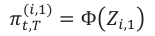
Here, Ȱ(Ǥ )stands for the cumulative distribution function for the standard Gaussian.
The approach of assuming that transitions between several discrete states are driven by a latent variable with a continuous distribution is widely applied in the discrete choice econometrics literature. When the latent variable is normally distributed, it corresponds to the ordered probit approach. The major benefit of employing this approach in credit risk modelling is that it permits one to allow rating transitions by different obligors to be correlated simply by assuming that the latent variables driving transitions for different credit exposures are correlated.
The model assumes that the latent variable for the ݅_{tℎ} exposure ܣ_i can be broken down into an idiosyncratic component ݁_i and multiple systematic risk factors. All the factors are rescaled so that they have unit variance and a zero mean. For this study, we only use a region factor, ܨ_i. The model simulates random shocks to the idiosyncratic and systematic factors and these translate into shocks to the latent variable ܣ_i via a weighted sum: (4.2)

These capital resource figures may be compared with the required capital estimates presented in the middle (VaR estimates) and lower (ES estimates) blocks of the two tables. A conservative confidence level is 1 basis point. This may be thought of as a ‘AAA confidence level’ since banks that aim for extremely high credit quality commonly use confidence levels in this region. The confidence level to which Basel II and III capital charges are calibrated is 10 basis points with a 1-year VaR horizon. It is also conservative and advisable to allow for randomness in LGDs.[20]
The 1-year horizon, 1 bps VaR capital estimate, inclusive of LGD risk, for IBRD is $17.7 bn. This estimate employs parameters (PDs and mean LGDs) adjusted for PCT. When non-PCT-adjusted parameters are employed, the estimate rises to $62.4 bn. The PCT adjustments draw on analysis Risk Control performed for the G20 CAF Panel, see Risk Control (2022a). This showed that PCT reduces LGD means and PDs compared to the values one may estimate using public bond market data each by more than 3 times.
The equivalent figures from Table 4.2 which presents results using a 3-year horizon for VaR and ES calculations are $23.3 bn and $78.3 bn. Some MDBs use a risk horizon of 3-years in contrast to the 1-year horizon that is typical among large commercial banks (and which is required in the Basel rules) to achieve greater conservatism. We would tend to regard the 1-year horizon results as the primary base case although use of a 3year horizon by non-regulated entities like MDBs is not unreasonable.
Turning to the results for IDA, on finds from Table 4.1 that the 1 basis point, 1-year-horizon VaR-based capital estimate inclusive of PCT and LGD risk is $22.2 bn. If one employs a 3-year horizon (see Table 4.2), the required capital estimate for IDA is $27.5 bn.
The capital required may be compared to the capital resources shown in the upper parts of Tables 4.1 and 4.2. To repeat, the base case credit risk EC for IBRD and IDA are, respectively, $17.7 bn and $22.2 bn. These may be compared with the Total Capital for the two institutions of $55.3 bn for IBRD and $178.7 bn for IDA. When Eligible Callable Capital is added to IBRD Total Equity, one obtains Adjusted Capital of $97.4 bn. One may consider scaling up the credit risk EC to obtain an approximate total EC. One may further boost EC by 10% to allow for a crisis buffer. The resulting estimate of total EC would be around $22 bn for IBRD or $27 bn for IDA. These are clearly a small fraction of the capital resources of the two institutions.
As a sensitivity analysis, we calculated an alternative transition matrix in which the righthand column of PDs is directly estimated from MDB historical non-accrual data of the MDBs. The results are given in Table 4.3. The capital numbers are generally slightly lower than those we obtained using the base case calibration.
As a second sensitivity analysis, we estimated a factor correlation matrix using correlations of sovereign bond spreads for different regions. The results are given in Table 4.4. Again, the capital numbers are somewhat lower than the base case results.
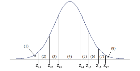
| >' Ɛ | >' Ɛ | >' Ɛ | >' Ɛ | >' Ɛ | >' Ɛ | >' Ɛ | >' Ɛ | |
|---|---|---|---|---|---|---|---|---|
| dŽƚĂů ĞdžƉŽƐƵƌĞ | Ϯϲϲ͕ϲϬϲ | Ϯϭϯ͕ϰϬϰ | ||||||
| dŽƚĂů ĞƋƵŝƚLJ | ϱϱ͕ϯϮϬ | ϭϳϴ͕ϲϲϴ | ||||||
| ůŝŐŝďůĞ ĐĂůůĂďůĞ ĐĂƉŝƚĂů | ϰϮ͕ϬϲϮ | Ϭ | ||||||
| ĚũƵƐƚĞĚ ĐĂƉŝƚĂů ; Ϳ | ϵϳ͕ϯϴϮ | ϭϳϴ͕ϲϲϴ | ||||||
| sĂZ ϭϬďƉ | ϲ͕Ϭϲϳ | ϭϬ͕ϵϰϳ | ϯϲ͕ϭϳϮ | ϯϵ͕ϳϰϬ | ϴ͕ϴϰϭ | ϭϰ͕ϵϵϴ | ϰϴ͕ϲϵϳ | ϱϰ͕ϯϭϯ |
| sĂZ ϯďƉ | ϳ͕ϵϰϵ | ϭϯ͕ϵϰϵ | ϰϲ͕ϳϵϳ | ϱϭ͕ϮϬϵ | ϭϬ͕ϳϬϵ | ϭϴ͕ϳϳϳ | ϱϳ͕Ϭϴϲ | ϲϰ͕ϭϴϵ |
| sĂZ ϭďƉ | ϵ͕ϵϴϰ | ϭϳ͕ϳϯϴ | ϱϲ͕ϱϳϱ | ϲϮ͕ϯϳϭ | ϭϮ͕ϱϮϱ | ϮϮ͕Ϯϭϯ | ϲϰ͕ϬϬϳ | ϳϮ͕ϭϭϳ |
| sĂZ ϭϬďƉ й ŽĨ | ϲ͘Ϯϯй | ϭϭ͘Ϯϰй | ϯϳ͘ϭϰй | ϰϬ͘ϴϭй | ϰ͘ϵϱй | ϴ͘ϯϵй | Ϯϳ͘Ϯϲй | ϯϬ͘ϰϬй |
| sĂZ ϯďƉ й ŽĨ | ϴ͘ϭϲй | ϭϰ͘ϯϮй | ϰϴ͘Ϭϱй | ϱϮ͘ϱϵй | ϱ͘ϵϵй | ϭϬ͘ϱϭй | ϯϭ͘ϵϱй | ϯϱ͘ϵϯй |
| sĂZ ϭďƉ й ŽĨ | ϭϬ͘Ϯϱй | ϭϴ͘Ϯϭй | ϱϴ͘ϭϬй | ϲϰ͘Ϭϱй | ϳ͘Ϭϭй | ϭϮ͘ϰϯй | ϯϱ͘ϴϮй | ϰϬ͘ϯϲй |
| ^ ϭϬďƉ | ϳ͕ϳϬϭ | ϭϯ͕ϲϴϴ | ϰϱ͕Ϭϯϱ | ϰϵ͕ϯϱϲ | ϭϬ͕ϰϯϯ | ϭϴ͕ϭϬϲ | ϱϱ͕ϯϰϯ | ϲϮ͕Ϭϳϲ |
| ^ ϯďƉ | ϵ͕ϴϲϵ | ϭϳ͕ϯϯϭ | ϱϲ͕ϯϬϴ | ϲϭ͕ϲϰϳ | ϭϮ͕ϯϰϰ | Ϯϭ͕ϴϬϳ | ϲϮ͕ϴϵϴ | ϳϭ͕Ϭϵϯ |
| ^ ϭďƉ | ϭϮ͕ϬϴϬ | Ϯϭ͕ϭϬϭ | ϲϲ͕ϳϮϬ | ϳϯ͕ϯϱϵ | ϭϰ͕Ϭϴϵ | Ϯϰ͕ϴϭϲ | ϲϴ͕ϳϱϬ | ϳϴ͕ϰϵϳ |
| ^ ϭϬďƉ й ŽĨ | ϳ͘ϵϭй | ϭϰ͘Ϭϲй | ϰϲ͘Ϯϱй | ϱϬ͘ϲϴй | ϱ͘ϴϰй | ϭϬ͘ϭϯй | ϯϬ͘ϵϴй | ϯϰ͘ϳϰй |
| ^ ϯďƉ й ŽĨ | ϭϬ͘ϭϯй | ϭϳ͘ϴϬй | ϱϳ͘ϴϮй | ϲϯ͘ϯϬй | ϲ͘ϵϭй | ϭϮ͘Ϯϭй | ϯϱ͘ϮϬй | ϯϵ͘ϳϵй |
| ^ ϭďƉ й ŽĨ | ϭϮ͘ϰϬй | Ϯϭ͘ϲϳй | ϲϴ͘ϱϭй | ϳϱ͘ϯϯй | ϳ͘ϴϵй | ϭϯ͘ϴϵй | ϯϴ͘ϰϴй | ϰϯ͘ϵϯй |
Note: Eligible callable capital is the callable capital from the AAA-rated countries and adjusted capital is the sum of total equity and eligible callable capital.
| >' Ɛ | >' Ɛ | >' Ɛ | >' Ɛ | >' Ɛ | >' Ɛ | >' Ɛ | >' Ɛ | |
|---|---|---|---|---|---|---|---|---|
| dŽƚĂů ĞdžƉŽƐƵƌĞ | Ϯϲϲ͕ϲϬϲ | Ϯϭϯ͕ϰϬϰ | ||||||
| dŽƚĂů ĞƋƵŝƚLJ | ϱϱ͕ϯϮϬ | ϭϳϴ͕ϲϲϴ | ||||||
| ůŝŐŝďůĞ ĐĂůůĂďůĞ ĐĂƉŝƚĂů | ϰϮ͕ϬϲϮ | Ϭ | ||||||
| ĚũƵƐƚĞĚ ĐĂƉŝƚĂů ; Ϳ | ϵϳ͕ϯϴϮ | ϭϳϴ͕ϲϲϴ | ||||||
| sĂZ ϭϬďƉ | ϴ͕ϵϵϳ | ϭϱ͕Ϭϰϱ | ϱϬ͕ϵϰϱ | ϱϱ͕ϵϳϮ | ϭϭ͕ϭϲϳ | ϭϵ͕ϰϯϲ | ϱϯ͕ϰϳϰ | ϲϭ͕ϱϵϬ |
| sĂZ ϯďƉ | ϭϭ͕ϯϯϳ | ϭϵ͕ϮϰϬ | ϲϮ͕ϴϯϭ | ϲϴ͕ϳϭϮ | ϭϯ͕Ϭϳϱ | Ϯϯ͕ϴϯϳ | ϲϬ͕ϬϵϮ | ϳϬ͕ϲϭϭ |
| sĂZ ϭďƉ | ϭϯ͕ϳϭϱ | Ϯϯ͕Ϯϱϲ | ϳϭ͕Ϭϲϳ | ϳϴ͕Ϯϱϴ | ϭϰ͕ϳϱϲ | Ϯϳ͕ϱϯϵ | ϲϱ͕ϮϰϬ | ϳϳ͕ϳϱϵ |
| sĂZ ϭϬďƉ й ŽĨ | ϵ͘Ϯϰй | ϭϱ͘ϰϱй | ϱϮ͘ϯϭй | ϱϳ͘ϰϴй | ϲ͘Ϯϱй | ϭϬ͘ϴϴй | Ϯϵ͘ϵϯй | ϯϰ͘ϰϳй |
| sĂZ ϯďƉ й ŽĨ | ϭϭ͘ϲϰй | ϭϵ͘ϳϲй | ϲϰ͘ϱϮй | ϳϬ͘ϱϲй | ϳ͘ϯϮй | ϭϯ͘ϯϰй | ϯϯ͘ϲϯй | ϯϵ͘ϱϮй |
| sĂZ ϭďƉ й ŽĨ | ϭϰ͘Ϭϴй | Ϯϯ͘ϴϴй | ϳϮ͘ϵϴй | ϴϬ͘ϯϲй | ϴ͘Ϯϲй | ϭϱ͘ϰϭй | ϯϲ͘ϱϭй | ϰϯ͘ϱϮй |
| ^ ϭϬďƉ | ϭϬ͕ϵϲϰ | ϭϴ͕ϱϰϮ | ϲϬ͕Ϯϳϲ | ϲϲ͕ϭϭϭ | ϭϮ͕ϳϮϵ | ϮϮ͕ϵϳϳ | ϱϴ͕ϲϯϬ | ϲϴ͕ϴϭϵ |
| ^ ϯďƉ | ϭϯ͕ϰϬϰ | ϮϮ͕ϴϳϰ | ϳϬ͕ϱϵϰ | ϳϴ͕ϬϭϬ | ϭϰ͕ϰϰϮ | Ϯϳ͕ϭϯϳ | ϲϯ͕ϵϴϵ | ϳϲ͕ϴϲϬ |
| ^ ϭďƉ | ϭϱ͕ϱϰϴ | Ϯϲ͕ϳϬϲ | ϳϵ͕ϭϯϯ | ϴϴ͕ϱϮϰ | ϭϱ͕ϴϳϭ | ϯϬ͕ϲϳϮ | ϲϳ͕ϱϳϮ | ϴϯ͕ϰϵϴ |
| ^ ϭϬďƉ й ŽĨ | ϭϭ͘Ϯϲй | ϭϵ͘Ϭϰй | ϲϭ͘ϵϬй | ϲϳ͘ϴϵй | ϳ͘ϭϮй | ϭϮ͘ϴϲй | ϯϮ͘ϴϭй | ϯϴ͘ϱϮй |
| ^ ϯďƉ й ŽĨ | ϭϯ͘ϳϲй | Ϯϯ͘ϰϵй | ϳϮ͘ϰϵй | ϴϬ͘ϭϭй | ϴ͘Ϭϴй | ϭϱ͘ϭϵй | ϯϱ͘ϴϭй | ϰϯ͘ϬϮй |
| ^ ϭďƉ й ŽĨ | ϭϱ͘ϵϳй | Ϯϳ͘ϰϮй | ϴϭ͘Ϯϲй | ϵϬ͘ϵϬй | ϴ͘ϴϴй | ϭϳ͘ϭϳй | ϯϳ͘ϴϮй | ϰϲ͘ϳϯй |
Note: Eligible callable capital is the callable capital from the AAA-rated countries and adjusted capital is the sum of total equity and eligible callable capital.
| >' Ɛ | >' Ɛ | >' Ɛ | >' Ɛ | >' Ɛ | >' Ɛ | >' Ɛ | >' Ɛ | |
|---|---|---|---|---|---|---|---|---|
| sĂZ ϭϬďƉ | ϱ͕ϱϰϵ | ϵ͕Ϭϰϭ | ϲ͕ϲϬϱ | ϭϭ͕ϯϮϵ | ϴ͕ϬϯϬ | ϭϮ͕ϳϴϳ | ϴ͕ϴϳϱ | ϭϱ͕ϬϱϬ |
| sĂZ ϯďƉ | ϳ͕ϵϵϰ | ϭϯ͕ϬϭϬ | ϴ͕ϵϰϲ | ϭϱ͕ϬϲϬ | ϭϬ͕ϴϯϴ | ϭϳ͕ϯϭϬ | ϭϭ͕Ϭϵϯ | ϭϴ͕ϵϴϲ |
| sĂZ ϭďƉ | ϭϬ͕ϱϱϬ | ϭϲ͕ϵϯϱ | ϭϭ͕ϭϬϲ | ϭϴ͕ϭϱϯ | ϭϯ͕ϲϱϲ | Ϯϭ͕ϱϮϰ | ϭϯ͕ϭϮϭ | Ϯϯ͕ϭϴϯ |
| sĂZ ϭϬďƉ й ŽĨ | ϱ͘ϳϬй | ϵ͘Ϯϴй | ϯ͘ϳϬй | ϲ͘ϯϰй | ϴ͘Ϯϱй | ϭϯ͘ϭϯй | ϰ͘ϵϳй | ϴ͘ϰϮй |
| sĂZ ϯďƉ й ŽĨ | ϴ͘Ϯϭй | ϭϯ͘ϯϲй | ϱ͘Ϭϭй | ϴ͘ϰϯй | ϭϭ͘ϭϯй | ϭϳ͘ϳϳй | ϲ͘Ϯϭй | ϭϬ͘ϲϯй |
| sĂZ ϭďƉ й ŽĨ | ϭϬ͘ϴϯй | ϭϳ͘ϯϵй | ϲ͘ϮϮй | ϭϬ͘ϭϲй | ϭϰ͘ϬϮй | ϮϮ͘ϭϬй | ϳ͘ϯϰй | ϭϮ͘ϵϴй |
| ^ ϭϬďƉ | ϳ͕ϲϳϭ | ϭϮ͕ϯϰϭ | ϴ͕ϱϰϱ | ϭϰ͕ϯϵϰ | ϭϬ͕ϯϱϭ | ϭϲ͕ϱϱϱ | ϭϬ͕ϳϬϮ | ϭϴ͕ϰϬϳ |
| ^ ϯďƉ | ϭϬ͕ϰϰϯ | ϭϲ͕ϳϱϬ | ϭϬ͕ϵϰϱ | ϭϴ͕ϬϬϰ | ϭϯ͕ϯϭϳ | Ϯϭ͕ϰϱϳ | ϭϮ͕ϴϯϭ | ϮϮ͕ϲϲϮ |
| ^ ϭďƉ | ϭϯ͕Ϭϳϲ | Ϯϭ͕ϭϬϳ | ϭϯ͕ϭϬϬ | Ϯϭ͕Ϭϵϰ | ϭϲ͕ϬϬϰ | Ϯϲ͕Ϭϳϴ | ϭϰ͕ϳϲϮ | Ϯϲ͕ϲϱϱ |
| ^ ϭϬďƉ й ŽĨ | ϳ͘ϴϴй | ϭϮ͘ϲϳй | ϰ͘ϳϴй | ϴ͘Ϭϲй | ϭϬ͘ϲϯй | ϭϳ͘ϬϬй | ϱ͘ϵϵй | ϭϬ͘ϯϬй |
| ^ ϯďƉ й ŽĨ | ϭϬ͘ϳϮй | ϭϳ͘ϮϬй | ϲ͘ϭϯй | ϭϬ͘Ϭϴй | ϭϯ͘ϲϳй | ϮϮ͘Ϭϯй | ϳ͘ϭϴй | ϭϮ͘ϲϴй |
| ^ ϭďƉ й ŽĨ | ϭϯ͘ϰϯй | Ϯϭ͘ϲϳй | ϳ͘ϯϯй | ϭϭ͘ϴϭй | ϭϲ͘ϰϯй | Ϯϲ͘ϳϴй | ϴ͘Ϯϲй | ϭϰ͘ϵϮй |
| >' Ɛ | >' Ɛ | >' Ɛ | >' Ɛ | >' Ɛ | >' Ɛ | >' Ɛ | >' Ɛ | |
|---|---|---|---|---|---|---|---|---|
| sĂZ ϭϬďƉ | ϰ͕ϱϵϱ | ϵ͕ϳϴϵ | ϵ͕ϵϴϵ | ϭϲ͕ϭϬϲ | ϲ͕ϰϴϯ | ϭϯ͕ϯϴϳ | ϭϭ͕ϵϬϵ | ϮϬ͕ϰϲϲ |
| sĂZ ϯďƉ | ϱ͕ϳϰϰ | ϭϮ͕ϭϴϱ | ϭϭ͕ϴϲϵ | ϮϬ͕ϮϭϮ | ϳ͕ϵϭϴ | ϭϲ͕ϱϲϯ | ϭϯ͕ϱϮϮ | Ϯϰ͕ϱϭϭ |
| sĂZ ϭďƉ | ϲ͕ϴϰϮ | ϭϰ͕ϱϭϰ | ϭϯ͕ϭϲϮ | Ϯϯ͕ϴϵϭ | ϵ͕ϮϮϱ | ϭϵ͕ϴϭϰ | ϭϰ͕ϳϬϯ | Ϯϴ͕ϭϬϳ |
| sĂZ ϭϬďƉ й ŽĨ | ϰ͘ϳϮй | ϭϬ͘Ϭϱй | ϱ͘ϱϵй | ϵ͘Ϭϭй | ϲ͘ϲϲй | ϭϯ͘ϳϱй | ϲ͘ϲϳй | ϭϭ͘ϰϱй |
| sĂZ ϯďƉ й ŽĨ | ϱ͘ϵϬй | ϭϮ͘ϱϭй | ϲ͘ϲϰй | ϭϭ͘ϯϭй | ϴ͘ϭϯй | ϭϳ͘Ϭϭй | ϳ͘ϱϳй | ϭϯ͘ϳϮй |
| sĂZ ϭďƉ й ŽĨ | ϳ͘Ϭϯй | ϭϰ͘ϵϬй | ϳ͘ϯϳй | ϭϯ͘ϯϳй | ϵ͘ϰϳй | ϮϬ͘ϯϱй | ϴ͘Ϯϯй | ϭϱ͘ϳϯй |
| ^ ϭϬďƉ | ϱ͕ϱϱϴ | ϭϭ͕ϳϳϰ | ϭϭ͕ϰϳϳ | ϭϵ͕ϰϮϱ | ϳ͕ϲϳϭ | ϭϲ͕ϭϭϯ | ϭϯ͕ϭϯϵ | Ϯϯ͕ϴϮϳ |
| ^ ϯďƉ | ϲ͕ϳϴϯ | ϭϰ͕ϰϮϰ | ϭϯ͕ϭϴϮ | Ϯϯ͕ϱϳϰ | ϵ͕ϭϬϰ | ϭϵ͕ϱϱϮ | ϭϰ͕ϱϴϴ | Ϯϳ͕ϳϵϴ |
| ^ ϭďƉ | ϴ͕Ϭϭϯ | ϭϲ͕ϵϵϭ | ϭϰ͕ϲϰϯ | Ϯϳ͕ϭϲϴ | ϭϬ͕ϰϬϯ | ϮϮ͕ϵϱϱ | ϭϱ͕ϳϭϰ | ϯϭ͕ϰϭϮ |
| ^ ϭϬďƉ й ŽĨ | ϱ͘ϳϭй | ϭϮ͘Ϭϵй | ϲ͘ϰϮй | ϭϬ͘ϴϳй | ϳ͘ϴϴй | ϭϲ͘ϱϱй | ϳ͘ϯϱй | ϭϯ͘ϯϰй |
| ^ ϯďƉ й ŽĨ | ϲ͘ϵϳй | ϭϰ͘ϴϭй | ϳ͘ϯϴй | ϭϯ͘ϭϵй | ϵ͘ϯϱй | ϮϬ͘Ϭϴй | ϴ͘ϭϳй | ϭϱ͘ϱϲй |
| ^ ϭďƉ й ŽĨ | ϴ͘Ϯϯй | ϭϳ͘ϰϱй | ϴ͘ϮϬй | ϭϱ͘Ϯϭй | ϭϬ͘ϲϴй | Ϯϯ͘ϱϳй | ϴ͘ϳϵй | ϭϳ͘ϱϴй |
4.4 Buffer Analysis
In this subsection, we display the VaR results when the sovereign ratings are downgraded in line with a worstcase crisis scenario. Appendix 8 provides more details of how this scenario is constructed but, in brief, it combines the sovereign rating downgrades that occurred both in the Covid 19 crisis and the Global Financial Crisis of 2007-9.
| / Z / | |||||||
|---|---|---|---|---|---|---|---|
| EŽŶͲƐƚŽĐŚĂƐƚŝĐ >' Ɛ | ^ƚŽĐŚĂƐƚŝĐ >' Ɛ | EŽŶͲƐƚŽĐŚĂƐƚŝĐ >' Ɛ | ^ƚŽĐŚĂƐƚŝĐ >' Ɛ | ||||
| sĂZ ϭϬďƉ ϲ͕ϯϳϲ | ϭϭ͕Ϯϲϭ | ϵ͕ϰϮϬ ϭϲ͕ϳϲϵ | |||||
| sĂZ ϯďƉ ϴ͕ϯϭϭ | ϭϰ͕ϭϭϭ | ϭϭ͕ϭϲϵ ϮϬ͕ϲϮϵ | |||||
| sĂZ ϭďƉ ϭϬ͕ϯϬϮ | ϭϳ͕ϴϴϲ | ϭϮ͕ϵϭϴ Ϯϯ͕ϴϬϬ | |||||
| sĂZ ϭϬďƉ й ŽĨ ϲ͘ϱϱй | ϭϭ͘ϱϲй | ϱ͘Ϯϳй ϵ͘ϯϵй | |||||
| sĂZ ϯďƉ й ŽĨ ϴ͘ϱϯй | ϭϰ͘ϰϵй | ϲ͘Ϯϱй ϭϭ͘ϱϱй | |||||
| sĂZ ϭďƉ й ŽĨ ϭϬ͘ϱϴй | ϭϴ͘ϯϳй | ϳ͘Ϯϯй ϭϯ͘ϯϮй | |||||
| ŚĂŶŐĞ ĨƌŽŵ ďĂƐĞ sĂZ ϭϬďƉ | ϱ͘Ϭϵй | Ϯ͘ϴϲй | ϲ͘ϱϱй ϭϭ͘ϴϭй | ||||
| ŚĂŶŐĞ ĨƌŽŵ ďĂƐĞ sĂZ ϯďƉ | ϰ͘ϱϲй | ϭ͘ϭϲй | ϰ͘Ϯϵй ϵ͘ϴϲй | ||||
| ŚĂŶŐĞ ĨƌŽŵ ďĂƐĞ sĂZ ϭďƉ | ϯ͘ϭϵй | Ϭ͘ϴϰй | ϯ͘ϭϯй ϳ͘ϭϱй |
5. Sustainable Concessional Lending Limit
5.1 Introduction
This section explains the constraint on IDA lending attributable to its use of concessional loans. We term this constraint the Sustainable Concessional Lending Limit (SCLL). A development institution can sustainably lend on a zero-interest-rate basis up to value of its capital so long as it can cover its costs and is not required to pay dividends.
Whenever a zero-interest-rate loan matures and is repaid, the lender may extend a new zero interest rate loan in the same amount. IDA charges borrowers a fee of 75 basis points but no interest rate which appears to cover the institution’s costs and is not required dividends.
IDA indeed currently lends an amount approximately equal to its capital, but this lending includes (i) nonconcessional loans, (ii) so-called blended loans and (iii) fully concessional (zero-interest-rate) loans. Blended loans have relatively low but still non-zero interest rates.
In this section, we calculate the headroom that IDA has available to increase its lending, allowing for the subsidy elements in much of its lending. To do this, we calculate the amounts of fully concessional and fully non-concessional loans that are equivalent to a dollar of blended lending.
We argue that the non-concessional lending is unconstrained since the institution’s available capital is sufficient to borrow extensively in capital markets. The sum of IDA’s fully concessional lending and the concessional component of its blended loans is less than its capital which creates room to lend more either through more concessional or more blended loans.
5.2 IDA Portfolio
Figure 5.1 shows the breakdown of IDA lending as it stood at end-June 2022 (see Panel a)) and the same breakdown for loans made in the IDA 19 replenishment period (see Panel b)).
The figure suggests that IDA's split of activities has shifted towards blended lending. Blended loans accounted for 38% of the entire loan portfolio at the end of June 2022 (see Panel a)). In the IDA19 replenishment period, however, blended loans represented 56% of total loans approved (see Panel b)). Non-concessional loans comprised 4% of the end-June 2022 portfolio, whereas they made up 9% of approvals in the IDA19 period.
The analysis presented in this note examines the headroom that IDA has available to change its different categories of lending given the constraint it faces as a concessional lender. For an institution to make zerointerest-rate loans sustainably (i.e., in a way that permits it to maintain the same volume of lending indefinitely), it cannot exceed the institution’s equity (in IDA’s case, $179 bn).
To understand this, suppose that IDA lends $100 for zero interest and then re-lends the same amount after the money is repaid again at zero interest. IDA will never receive a return on the activity. So, the present value of this activity is zero. Thus, a limit on IDA's sustainable, fully concessional lending is the institution’s equity. Here, we assume their periodic injections of donor cash are used up in grants and that other sources of income, notably IDA’s administration charge to borrowers of 75 bps covers its operational costs.
At the end of June 2022, IDA had $105 bn of concessional loans, $66 bn of blended and $6 bn of nonconcessional, so $178 bn in total. On the face of it, this does leave IDA with the possibility of lending more. The amount of capital available to IDA means that it could borrow extensively in the capital markets and make nonconcessional lending. Blended loans may be thought of as a combination of concessional and non-concessional. In the next section, we break down IDA’s $66 bn of blended loans into (a) fully concessional and (b) fully nonconcessional loans with market and par values that sum to equal, respectively, the market and par values of the original blended loans.
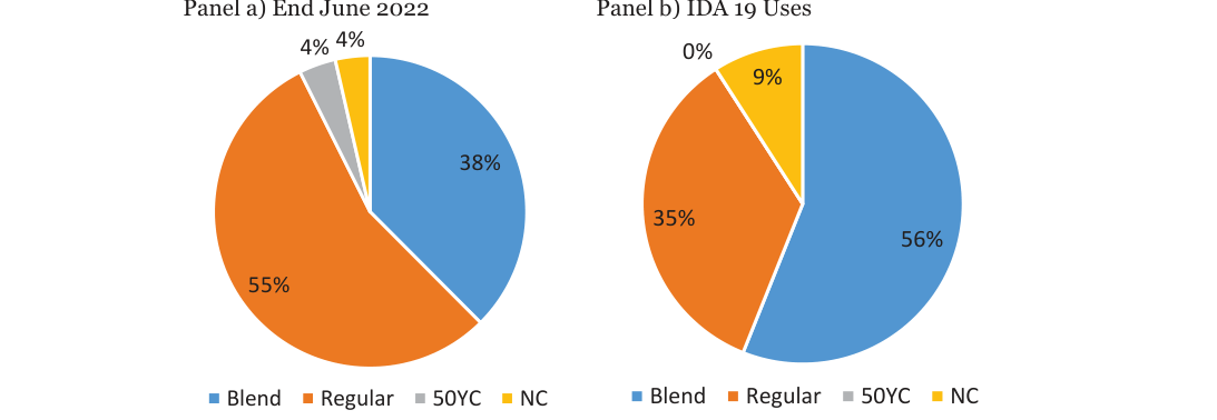
Note: Panel a) is based on the historical data of ‘IDA Statement of Credits and Grants.’ Panel b) is based on the funding allocation of IDA 19 described in IDA FY22 Management’s Discussion and Analysis. 50YC denotes 50-year credit, and NC indicates Non-Concessional.
5.3 Blended Loans
Suppose we have blended loans with a par value of $1. Can we split this into amount of concessional loans (LCs) and non-concessional loans (NCLs) that are equivalent in the sense that the sums of (i) the par values and (ii) the market values of the CLs and NCLs are equal to those of the blended loan with $1 par. This is our topic in this section.

split these as follows:
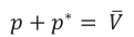
(5.1) ݒ+ݒכ =ܸ
Here, p and v are the par value and fair value, respectively, of the CLs and כ and ݒכ are the par value and fair value of the NCLs.
The par value (כ) of the NCL must equal its market value (ݒכ). On subtracting the two equations in equation (5.1), and rearranging we obtain: (5.2)
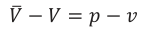
In equation (5.2), the fair value of the CL depends implicitly on its par value, so one may consider v to be a function of p. We compute p by finding the value such that equation (5.2) is satisfied. One may understand this

concessional part of the blended loans (i.e., −ݒ ).

We take the blended loan portfolio and compute the present value of the portfolio assuming all the blended

loans are lent at zero interest rate.[21] This exercise is repeated for various possible shares of the ratio of ߙؠ

from 0% to 100%.

Figure 5.2 shows that ߙؠ

the lending headroom.
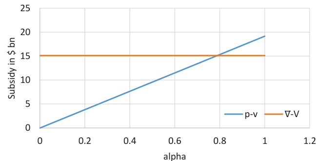
6. Risk Transfer Analysis
6.1 Introduction
MDBs are key institutions in the effort to achieve the Sustainable Development Goals (SDGs) proposed by the United Nations. Even if they increase their lending substantially, this will not alone produce the hundreds of billions required to attain the SDGs. The efficiency of MDB capital utilisation must be increased by risk transfer techniques that bring private and donor risk bearing capacity to bear. This section considers such transactions and examines constraints that may limit MDB risk transfer.
Risk-transfer transactions undertaken by MDBs in the past are discussed by Galizia et al. (2019). These include:
1. Portfolio exchanges between MDBs.
2. A landmark securitization of corporate loans by the African Development Bank (AfDB) (see Risk Control (2019)).
3. A series of financial transactions through which the European Commission has implemented (via the European Investment Bank—EIB) its Investment Plan for Europe.
4. Guarantees provided by the Swedish International Development Agency (SIDA) to the Inter-American Development Bank (IDB) and Asian Development Bank (ADB).
5. A further synthetic securitisation by the AfDB involving sovereign loans in which the protection providers included the UK’s Foreign, Commonwealth and Development Office (FCDO) and private sector insurers.
Since the CAF Panel report was published, many MDBs have started reviewing risk transfer transactions that they might implement. One such possible transaction that has been publicly discussed is the ADB’s Innovative Finance Facility for Climate in Asia and the Pacific (IF-CAP) (see ADB (2023)).
These techniques could further increase MDB lending when supported by a broader and deeper investor base. The nature of the protection providers varies according to the deal. In several, risk capacity is provided by donor governments or public entities. The AfDB transactions listed are particularly notable because, in both cases, private sector protection providers participated.
To assess the constraints that limit scope for risk transfer, in this section, we analyse synthetic securitisations involving IBRD and IDA portfolios of sovereign loans. For simplicity and concreteness, we consider transactions comparable to the AfDB’s Room2Run transaction (see Risk Control (2019)). While the precise structure might be adjusted, for simplicity, we suppose the same tranching as was used in the Room2Run transaction and that the MDB in each case retains the Junior and Senior tranches. The Mezzanine tranche is transferred to external institutions or investors.
We analyse: x the increase in the Standard & Poor’s RAC ratio that results from the transaction, x reduction in credit risk Economic Capital (EC), x estimate the tranche ratings using the Standard & Poor’s methodology, and x the fair value price of the mezzanine tranche following a securitisation of the portfolio and the fraction of spread income on the securitised portfolio that the MDB can achieve.
For each institution, we consider securitisations involving two portfolios. The two portfolios are denoted Portfolio A and Portfolio B, the first having the higher credit quality.
6.2 Description of a securitisation transaction
The tranche structure is described in Table 6.1.
We consider two different reference portfolios for the transaction. These are described in Tables 6.2 and 6.3. x Portfolio A consists of 15 exposures with the highest EAD and weights are adjusted to have a comparable weighted average rating with the overall portfolio. Table 6.2 shows the countries in Portfolio A with the exposure amounts and ratings. x Portfolio B consists of exposures with the highest 1bp Marginal Value-at-Risk (MVaR) values according to the results in Table 4.1 with PCT adjustments and non-stochastic LGDs. Top 30 exposures are chosen according to the marginal contributions they make to the Value of Risk associated with the MDB’s entire portfolio and these are further filtered by ratings. We choose exposures with ratings BB or below for IBRD and B and below for IDA. All the weights are chosen as 25% of the EADs for IBRD and 20% of the EADs for IDA. Weighted average ratings of the reference portfolios are B and B- for IBRD and IDA respectively. Table 6.3 shows the countries in Portfolio B with the exposure amounts and ratings.
| dƌĂŶĐŚĞƐ | ZĞƚĂŝŶĞĚ | ƚƚĂĐŚŵĞŶƚ WŽŝŶƚ | ĞƚĂĐŚŵĞŶƚ WŽŝŶƚ | dŚŝĐŬŶĞƐƐ |
|---|---|---|---|---|
| ^ĞŶŝŽƌ | zĞƐ | Ϯϳ͘Ϯϱй | ϭϬϬ͘ϬϬй | ϳϮ͘ϳϱй |
| ^ĞŶŝŽƌ DĞnjnjĂŶŝŶĞ | EŽ | ϭϳ͘Ϯϱй | Ϯϳ͘Ϯϱй | ϭϬ͘ϬϬй |
| :ƵŶŝŽƌ DĞnjnjĂŶŝŶĞ | EŽ | Ϯ͘ϬϬй | ϭϳ͘Ϯϱй | ϭϱ͘Ϯϱй |
| :ƵŶŝŽƌ | zĞƐ | Ϭ͘ϬϬй | Ϯ͘ϬϬй | Ϯ͘ϬϬй |
| KďůŝŐŽƌ | ZĂƚŝŶŐƐ | KďůŝŐŽƌ | ZĂƚŝŶŐƐ | KďůŝŐŽƌ | ZĂƚŝŶŐƐ | KďůŝŐŽƌ | ZĂƚŝŶŐƐ | ||||
|---|---|---|---|---|---|---|---|---|---|---|---|
| /ŶĚŝĂ | Ͳ | ϯ͕ϴϮϭ | WŚŝůŝƉƉŝŶĞƐ | н | ϭ͕ϳϴϲ | ĂŶŐůĂĚĞƐŚ | Ͳ | Ϯ͕ϭϵϰ | 'ŚĂŶĂ | Ͳ | ϭ͕ϭϳϰ |
| /ŶĚŽŶĞƐŝĂ | Ϯ͕ϭϴϱ | ƌŐĞŶƚŝŶĂ | Ɛ | Ϯ͕ϲϯϳ | /ŶĚŝĂ | Ͳ | Ϯ͕ϬϬϯ | hŐĂŶĚĂ | ϴϮϰ | ||
| ŚŝŶĂ | н | ϭ͕ϴϳϲ | DŽƌŽĐĐŽ | н | ϭ͕ϯϵϭ | WĂŬŝƐƚĂŶ | Ͳ | ϯ͕ϲϬϱ | EĞƉĂů | ϵϳϳ | |
| ƌĂnjŝů | Ͳ | ϯ͕ϰϯϰ | hŬƌĂŝŶĞ | Ɛ | ϭ͕Ϯϰϴ | EŝŐĞƌŝĂ | Ͳ | ϯ͕ϮϳϬ | ^ĞŶĞŐĂů | н | ϰϯϰ |
| DĞdžŝĐŽ | ϭ͕ϱϱϲ | WŽůĂŶĚ | Ͳ | ϵϰϵ | sŝĞƚŶĂŵ | н | ϭ͕ϰϬϱ | ƀƚĞ ĚΖ/ǀŽŝƌĞ | Ͳ | ϯϲϲ | |
| ŽůŽŵďŝĂ | н | Ϯ͕ϭϲϮ | ZŽŵĂŶŝĂ | Ͳ | ϴϮϳ | ƚŚŝŽƉŝĂ | Ɛ | ϭ͕ϵϭϰ | hnjďĞŬŝƐƚĂŶ | Ͳ | ϯϯϵ |
| ŐLJƉƚ | Ϯ͕Ϭϭϱ | WĞƌƵ | ϴϭϭ | <ĞŶLJĂ | ϭ͕ϳϵϬ | ^ƌŝ >ĂŶŬĂ | Ɛ | ϰϵϰ | |||
| dƺƌŬŝLJĞ | н | Ϯ͕ϲϲϭ | dĂŶnjĂŶŝĂ | ϭ͕ϱϳϵ | |||||||
| dŽƚĂů | Ϯϵ͕ϯϱϵ | ϮϮ͕ϯϲϴ |
| / Z | / | ||||||||||
|---|---|---|---|---|---|---|---|---|---|---|---|
| KďůŝŐŽƌ | ZĂƚŝŶŐƐ | KďůŝŐŽƌ | ZĂƚŝŶŐƐ | KďůŝŐŽƌ | ZĂƚŝŶŐƐ | KďůŝŐŽƌ | ZĂƚŝŶŐƐ | ||||
| ƌĂnjŝů | Ͳ | ϰ͕ϮϵϮ | 'ƵĂƚĞŵĂůĂ | Ͳ | ϱϬϰ | WĂŬŝƐƚĂŶ | Ͳ | ϯ͕ϲϬϱ | ƵƌŬŝŶĂ &ĂƐŽ | Ɛ | ϱϰϮ |
| ŐLJƉƚ | ϯ͕ϯϱϵ | 'ĞŽƌŐŝĂ | ϰϭϵ | EŝŐĞƌŝĂ | Ͳ | ϯ͕ϮϳϬ | EŝŐĞƌ | Ɛ | ϱϯϳ | ||
| dƵƌŬŝLJĞ | н | ϯ͕ϯϮϳ | ŽƐƚĂ ZŝĐĂ | ϰϬϰ | ƚŚŝŽƉŝĂ | Ɛ | Ϯ͕ϱϱϭ | DĂĚĂŐĂƐĐĂƌ | Ɛ | ϱϯϬ | |
| ƌŐĞŶƚŝŶĂ | Ɛ | Ϯ͕ϲϯϳ | ĞůĂƌƵƐ | Ɛ | Ϯϵϴ | <ĞŶLJĂ | Ϯ͕ϯϴϳ | DLJĂŶŵĂƌ | Ɛ | ϰϳϭ | |
| hŬƌĂŝŶĞ | Ɛ | Ϯ͕ϬϴϬ | ů ^ĂůǀĂĚŽƌ | Ɛ | Ϯϵϰ | dĂŶnjĂŶŝĂ | Ϯ͕ϭϬϲ | DĂůŝ | Ɛ | ϰϱϵ | |
| :ŽƌĚĂŶ | н | ϭ͕ϭϭϰ | >ĞďĂŶŽŶ | Ɛ | Ϯϲϲ | 'ŚĂŶĂ | Ͳ | ϭ͕ϭϳϰ | ĂŵďŝĂ | Ɛ | ϰϮϱ |
| dƵŶŝƐŝĂ | Ɛ | ϭ͕ϭϬϲ | ^ƌŝ >ĂŶŬĂ | Ɛ | Ϯϱϲ | hŐĂŶĚĂ | ϭ͕Ϭϵϵ | DĂůĂǁŝ | Ɛ | ϯϰϮ | |
| ĐƵĂĚŽƌ | Ͳ | ϭ͕Ϭϯϰ | ŽůŝǀŝĂ | н | Ϯϭϱ | EĞƉĂů | ϵϳϳ | zĞŵĞŶ | Ɛ | Ϯϱϱ | |
| /ƌĂƋ | Ͳ | ϵϱϯ | ^ƌŝ >ĂŶŬĂ | Ɛ | ϲϱϵ | >ĂŽƐ | Ɛ | ϭϵϴ | |||
| WĂŬŝƐƚĂŶ | Ͳ | ϵϮϯ | ĞŵŽĐƌĂƚŝĐ ZĞƉƵďůŝĐ | Ͳ | ϲϰϰ | EŝĐĂƌĂŐƵĂ | Ͳ | ϭϵϰ | |||
| ŽĨ ƚŚĞ ŽŶŐŽ | |||||||||||
| ŶŐŽůĂ | Ͳ | ϴϱϲ | DŽnjĂŵďŝƋƵĞ | Ɛ | ϲϭϮ | DŽŶŐŽůŝĂ | ϭϲϴ | ||||
| hnjďĞŬŝƐƚĂŶ | Ͳ | ϲϭϵ | ĂŵĞƌŽŽŶ | Ͳ | ϱϲϳ | ||||||
| dŽƚĂů | Ϯϰ͕ϵϱϲ | Ϯϯ͕ϳϳϭ |
6.3 RAC ratio impact of the securitisation
This subsection calculates the effect of the securitisation on the MDB’s RAC ratio and EC. Tables 6.4 and 6.5 shows the impact on the RAC ratios of IBRD and IDA, respectively. The RWAs associated with the retained Junior and Senior tranches are shown. Note that the RWAs for the senior tranche depend on the rating that the rating agency chooses to give to this tranche. The current Standard & Poor’s methodology for MDB retained senior tranches permits such tranches to obtain no more than a single-A rating. The methodology is based on a single-A stress implicit in the RAC framework used by the agency to rate MDBs. The methodology could easily be extended to permit AA or AAA ratings but currently this is not permitted by Standard & Poor’s. The tables show what the consequences would be in an increase in the efficiency of the transaction if the agency were persuaded to generalise its approach to permit other ratings.
The results show that with a securitisation representing 10% of the institution’s portfolio of sovereign loans, the RAC ratio increases from 25.96% to 27.45% in the case of the lower credit quality portfolio B for IBRD and to 26.68% when portfolio A is securitised. In the case of IDA, the gain in the RAC ratio is from a base value of 68.9% to 78.7% for portfolio B or to 80.9% in the case of portfolio A. These represent very substantial gains in the RAC ratio.
| ;ĂͿ | ;ďͿ | ||||||
|---|---|---|---|---|---|---|---|
| ZĞƐƵůƚƐ Ͱ ^ĐĞŶĂƌŝŽ | ĂƐĞ | ||||||
| 'ŽǀĞƌŶŵĞŶƚ ĂŶĚ ĐĞŶƚƌĂů ďĂŶŬƐ ĐƌĞĚŝƚ ƌŝƐŬ Zt | Ϯϵϱ͕ϰϯϴ | ϮϲϬ͕ϳϯϰ | ϮϲϬ͕ϳϯϰ | ϮϲϬ͕ϳϯϰ | Ϯϰϲ͕ϯϯϬ | Ϯϰϲ͕ϯϯϬ | Ϯϰϲ͕ϯϯϬ |
| ^ĞĐƵƌŝƚŝƐĂƚŝŽŶ Zt | Ϭ | ϭϯ͕ϰϱϰ | ϭϱ͕ϵϮϵ | ϮϬ͕ϴϳϴ | ϭϭ͕ϭϯϴ | ϭϯ͕ϭϴϲ | ϭϳ͕Ϯϴϰ |
| ^ĞĐƵƌŝƚŝƐĂƚŝŽŶ ^ƌ | Ϭ | ϰ͕ϵϱϬ | ϳ͕ϰϮϰ | ϭϮ͕ϯϳϰ | ϰ͕Ϭϵϳ | ϲ͕ϭϰϲ | ϭϬ͕Ϯϰϰ |
| ^ĞĐƵƌŝƚŝƐĂƚŝŽŶ :ƌ | Ϭ | ϴ͕ϱϬϰ | ϴ͕ϱϬϰ | ϴ͕ϱϬϰ | ϳ͕ϬϰϬ | ϳ͕ϬϰϬ | ϳ͕ϬϰϬ |
| dŽƚĂů ĐƌĞĚŝƚ ƌŝƐŬ Zt ďĞĨŽƌĞ ĂĚũƵƐƚŵĞŶƚƐ | ϯϬϲ͕Ϭϳϯ | Ϯϴϰ͕ϴϮϯ | Ϯϴϳ͕Ϯϵϳ | ϮϵϮ͕Ϯϰϳ | Ϯϴϲ͕ϭϬϭ | Ϯϴϴ͕ϭϰϵ | Ϯϳϰ͕Ϯϰϴ |
| 'ĞŽŐƌĂƉŚŝĐ ĐŽŶĐĞŶƚƌĂƚŝŽŶ ĂĚũƵƐƚŵĞŶƚ | Ͳϯϯ͕Ϯϵϲ | ͲϮϵ͕ϰϮϱ | ͲϮϵ͕ϰϮϱ | ͲϮϵ͕ϰϮϱ | ͲϮϵ͕Ϭϳϴ | ͲϮϵ͕Ϭϳϴ | ͲϮϵ͕Ϭϳϴ |
| ^ŝŶŐůĞ ŶĂŵĞ ĐŽŶĐĞŶƚƌĂƚŝŽŶ ĂĚũƵƐƚŵĞŶƚ | ϭϬϱ͕ϰϲϲ | ϴϳ͕Ϯϲϵ | ϴϳ͕Ϯϲϵ | ϴϳ͕Ϯϲϵ | ϵϳ͕ϵϰϴ | ϵϳ͕ϵϰϴ | ϵϳ͕ϵϰϴ |
| dŽƚĂů ĐƌĞĚŝƚ ƌŝƐŬ Zt ĂĨƚĞƌ ĂĚũƵƐƚŵĞŶƚƐ | Ϯϭϯ͕ϭϭϮ | ϭϵϵ͕ϵϱϰ | ϮϬϮ͕ϰϮϴ | ϮϬϳ͕ϯϳϴ | ϭϵϱ͕ϯϵϲ | ϭϵϳ͕ϰϰϱ | ϮϬϭ͕ϱϰϯ |
| dŽƚĂů ĞƋƵŝƚLJ | ϱϱ͕ϯϮϬ | ϱϱ͕ϯϮϬ | ϱϱ͕ϯϮϬ | ϱϱ͕ϯϮϬ | ϱϱ͕ϯϮϬ | ϱϱ͕ϯϮϬ | ϱϱ͕ϯϮϬ |
| Z ƌĂƚŝŽ | Ϯϱ͘ϵϲй | Ϯϳ͘ϲϳй | Ϯϳ͘ϯϯй | Ϯϲ͘ϲϴй | Ϯϴ͘ϯϭй | Ϯϴ͘ϬϮй | Ϯϳ͘ϰϱй |
Note: Portfolio (a) denotes the 10% securitization portfolio that is constituted by the top 15 loans. Portfolio (b) is constituted by the top 24 exposures with highest VaR.
| ;ĂͿ | ;ďͿ | ||||||
|---|---|---|---|---|---|---|---|
| ZĞƐƵůƚƐ Ͱ ^ĐĞŶĂƌŝŽ | ĂƐĞ | ||||||
| 'ŽǀĞƌŶŵĞŶƚ ĂŶĚ ĐĞŶƚƌĂů ďĂŶŬƐ ĐƌĞĚŝƚ ƌŝƐŬ Zt | Ϯϳϱ͕Ϯϯϰ | ϮϮϯ͕ϯϮϴ | ϮϮϯ͕ϯϮϴ | ϮϮϯ͕ϯϮϴ | Ϯϯϵ͕Ϭϯϭ | Ϯϯϵ͕Ϭϯϭ | Ϯϯϵ͕Ϭϯϭ |
| ^ĞĐƵƌŝƚŝƐĂƚŝŽŶ Zt | Ϭ | ϴ͕ϵϴϮ | ϭϬ͕ϲϯϰ | ϭϯ͕ϵϯϵ | ϭϬ͕Ϭϱϰ | ϭϭ͕ϵϬϯ | ϭϱ͕ϲϬϮ |
| ^ĞĐƵƌŝƚŝƐĂƚŝŽŶ ^ƌ | Ϭ | ϯ͕ϯϬϰ | ϰ͕ϵϱϳ | ϴ͕Ϯϲϭ | ϯ͕ϲϵϵ | ϱ͕ϱϰϴ | ϵ͕Ϯϰϳ |
| ^ĞĐƵƌŝƚŝƐĂƚŝŽŶ :ƌ | Ϭ | ϱ͕ϲϳϴ | ϱ͕ϲϳϴ | ϱ͕ϲϳϴ | ϲ͕ϯϱϱ | ϲ͕ϯϱϱ | ϲ͕ϯϱϱ |
| dŽƚĂů ĐƌĞĚŝƚ ƌŝƐŬ Zt ďĞĨŽƌĞ ĂĚũƵƐƚŵĞŶƚƐ | Ϯϴϲ͕ϱϯϯ | Ϯϰϭ͕Ϭϳϳ | ϮϰϮ͕ϳϮϵ | Ϯϰϲ͕Ϭϯϯ | Ϯϱϳ͕ϴϱϭ | Ϯϱϵ͕ϳϬϬ | Ϯϲϯ͕ϯϵϵ |
| 'ĞŽŐƌĂƉŚŝĐ ĐŽŶĐĞŶƚƌĂƚŝŽŶ ĂĚũƵƐƚŵĞŶƚ | ͲϮϭ͕ϮϮϬ | Ͳϭϳ͕ϬϬϬ | Ͳϭϳ͕ϬϬϬ | Ͳϭϳ͕ϬϬϬ | Ͳϭϵ͕ϭϲϭ | Ͳϭϵ͕ϭϲϭ | Ͳϭϵ͕ϭϲϭ |
| ^ŝŶŐůĞ ŶĂŵĞ ĐŽŶĐĞŶƚƌĂƚŝŽŶ ĂĚũƵƐƚŵĞŶƚ | ϭϬϮ͕ϱϴϱ | ϳϲ͕Ϭϱϰ | ϳϲ͕Ϭϱϰ | ϳϲ͕Ϭϱϰ | ϴϱ͕ϱϭϭ | ϴϱ͕ϱϭϭ | ϴϱ͕ϱϭϭ |
| dŽƚĂů ĐƌĞĚŝƚ ƌŝƐŬ Zt ĂĨƚĞƌ ĂĚũƵƐƚŵĞŶƚƐ | Ϯϱϵ͕ϰϯϲ | Ϯϭϲ͕ϬϭϬ | Ϯϭϳ͕ϲϲϮ | ϮϮϬ͕ϵϲϳ | ϮϮϭ͕ϰϳϭ | ϮϮϯ͕ϯϮϬ | ϮϮϳ͕Ϭϭϵ |
| dŽƚĂů ĞƋƵŝƚLJ | ϭϳϴ͕ϲϲϴ | ϭϳϴ͕ϲϲϴ | ϭϳϴ͕ϲϲϴ | ϭϳϴ͕ϲϲϴ | ϭϳϴ͕ϲϲϴ | ϭϳϴ͕ϲϲϴ | ϭϳϴ͕ϲϲϴ |
| Z ƌĂƚŝŽ | ϲϴ͘ϵй | ϴϮ͘ϳй | ϴϮ͘ϭй | ϴϬ͘ϵй | ϴϬ͘ϳй | ϴϬ͘Ϭй | ϳϴ͘ϳй |
Note: Portfolio (a) denotes the 10% securitization portfolio that is constituted by the top 15 loans. Portfolio (b) is constituted by the top 24 exposures with highest VaR.
6.4 Economic capital impact of securitisation
This subsection presents the gains that can be achieved through reduced EC if the IBRD and IDA were to securitise portfolios A or B. The results for the two institutions are given in Table 6.6 and Table 6.7 respectively. The 1-basis-point, 1-year, stochastic-LGD, VaR-based EC for IBRD and IDA drop by 12.04% and 11.29%, respectively, for portfolio A and by 18.28% and 12.66%, respectively, for portfolio B. Again, these represent substantial reductions in EC, especially in the case of the riskier portfolio B securitisations.
| >' Ɛ | >' Ɛ | >' Ɛ | >' Ɛ | >' Ɛ | >' Ɛ | >' Ɛ | >' Ɛ | |
|---|---|---|---|---|---|---|---|---|
| sĂZ ϭϬďƉ | ϱ͕ϴϵϬ | ϵ͕ϲϴϳ | ϴ͕Ϯϱϲ | ϭϯ͕ϭϳϬ | ϴ͕ϰϮϭ | ϭϯ͕ϯϮϳ | ϭϬ͕Ϯϭϱ | ϭϲ͕ϵϳϴ |
| sĂZ ϯďƉ | ϳ͕ϱϰϴ | ϭϮ͕ϭϵϰ | ϵ͕ϵϱϲ | ϭϲ͕ϱϰϳ | ϭϬ͕ϱϭϱ | ϭϲ͕ϵϴϯ | ϭϭ͕ϴϵϮ | ϮϬ͕ϳϯϴ |
| sĂZ ϭďƉ | ϵ͕ϰϬϬ | ϭϱ͕ϲϬϯ | ϭϭ͕ϱϰϲ | ϭϵ͕ϳϬϱ | ϭϮ͕ϲϬϳ | ϮϬ͕Ϯϴϳ | ϭϯ͕ϰϭϮ | Ϯϰ͕Ϭϳϲ |
| ŚĂŶŐĞ ĨƌŽŵ ĂƐĞ sĂZ ϭϬďƉ | ͲϮ͘ϵϭй | Ͳϭϭ͘ϱϮй | Ͳϲ͘ϲϮй | ͲϭϮ͘ϭϵй | Ͳϲ͘ϰϬй | Ͳϭϭ͘ϰϮй | Ͳϴ͘ϱϯй | ͲϭϮ͘ϲϱй |
| ŚĂŶŐĞ ĨƌŽŵ ĂƐĞ sĂZ ϯďƉ | Ͳϱ͘Ϭϱй | ͲϭϮ͘ϱϴй | Ͳϳ͘Ϭϯй | Ͳϭϭ͘ϴϴй | Ͳϳ͘Ϯϱй | Ͳϭϭ͘ϳϯй | Ͳϵ͘Ϭϰй | Ͳϭϯ͘ϬϬй |
| ŚĂŶŐĞ ĨƌŽŵ ĂƐĞ sĂZ ϭďƉ | Ͳϱ͘ϴϱй | ͲϭϮ͘Ϭϰй | Ͳϳ͘ϴϮй | Ͳϭϭ͘Ϯϵй | Ͳϴ͘Ϭϴй | ͲϭϮ͘ϳϳй | Ͳϵ͘ϭϭй | ͲϭϮ͘ϱϳй |
| ^ ϭϬďƉ | ϳ͕ϯϰϮ | ϭϮ͕Ϭϰϰ | ϵ͕ϲϴϯ | ϭϱ͕ϵϭϰ | ϭϬ͕ϭϳϱ | ϭϲ͕ϯϳϯ | ϭϭ͕ϲϭϭ | ϮϬ͕Ϭϳϳ |
| ^ ϯďƉ | ϵ͕Ϯϴϭ | ϭϱ͕Ϯϭϯ | ϭϭ͕ϯϵϳ | ϭϵ͕ϭϴϮ | ϭϮ͕ϯϰϰ | ϮϬ͕ϭϱϰ | ϭϯ͕ϭϰϬ | Ϯϯ͕ϳϭϰ |
| ^ ϭďƉ | ϭϭ͕Ϯϰϯ | ϭϴ͕ϱϯϬ | ϭϮ͕ϵϰϵ | Ϯϭ͕ϳϮϯ | ϭϰ͕Ϯϰϭ | Ϯϯ͕ϲϯϴ | ϭϰ͕ϰϮϴ | Ϯϲ͕ϴϮϱ |
| ŚĂŶŐĞ ĨƌŽŵ ĂƐĞ ^ ϭϬďƉ | Ͳϰ͘ϲϲй | ͲϭϮ͘Ϭϭй | Ͳϳ͘ϭϵй | ͲϭϮ͘ϭϭй | Ͳϳ͘ϮϬй | Ͳϭϭ͘ϳϬй | Ͳϴ͘ϳϵй | ͲϭϮ͘ϲϮй |
| ŚĂŶŐĞ ĨƌŽŵ ĂƐĞ ^ ϯďƉ | Ͳϱ͘ϵϱй | ͲϭϮ͘ϮϮй | Ͳϳ͘ϲϳй | ͲϭϮ͘Ϭϰй | Ͳϳ͘ϵϭй | Ͳϭϭ͘ϴϵй | Ͳϵ͘ϬϮй | ͲϭϮ͘ϲϭй |
| ŚĂŶŐĞ ĨƌŽŵ ĂƐĞ ^ ϭďƉ | Ͳϲ͘ϵϯй | ͲϭϮ͘ϭϵй | Ͳϴ͘Ϭϵй | ͲϭϮ͘ϰϳй | Ͳϴ͘ϰϬй | Ͳϭϭ͘ϰϵй | Ͳϵ͘Ϭϵй | ͲϭϮ͘ϱϰй |
| :ƵŶŝŽƌ ƚƌĂŶĐŚĞ ƉĂƌ ǀĂůƵĞ | ϱϴϳ | ϱϴϳ | ϰϰϳ | ϰϰϳ | ϱϴϳ | ϱϴϳ | ϰϰϳ | ϰϰϳ |
| DsĂZ ϭďƉ | ϱϭϰ | ϲϴϵ | ϰϱϰ | ϲϬϬ | ϱϮϭ | ϭϮϭϴ | ϯϮϲ | ϳϰϳ |
| DsĂZ ϭďƉ й ŽĨ sĂZ ϭďƉ | ϱ͘ϰϳй | ϰ͘ϰϮй | ϯ͘ϵϯй | ϯ͘Ϭϰй | ϰ͘ϭϯй | ϲ͘ϬϬй | Ϯ͘ϰϯй | ϯ͘ϭϬй |
| DsĂZ ϭďƉ й ŽĨ ƉĂƌ ǀĂůƵĞ | ϴϳ͘ϱϳй | ϭϭϳ͘ϯϱй | ϭϬϭ͘ϰϳй | ϭϯϰ͘Ϭϴй | ϴϴ͘ϳϯй | ϮϬϳ͘ϰϱй | ϳϮ͘ϳϴй | ϭϲϳ͘ϬϮй |
| ^ĞŶŝŽƌ ƚƌĂŶĐŚĞ ƉĂƌ ǀĂůƵĞ | Ϯϭ͕ϯϱϴ | Ϯϭ͕ϯϱϴ | ϭϲ͕Ϯϳϯ | ϭϲ͕Ϯϳϯ | Ϯϭ͕ϯϱϴ | Ϯϭ͕ϯϱϴ | ϭϲ͕Ϯϳϯ | ϭϲ͕Ϯϳϯ |
| DsĂZ ϭďƉ | Ϭ | Ϭ | Ϭ | Ϭ | Ϭ | Ϭ | Ϭ | ϱϰϵ |
| DsĂZ ϭďƉ й ŽĨ sĂZ ϭďƉ | Ϭ͘ϬϬй | Ϭ͘ϬϬй | Ϭ͘ϬϬй | Ϭ͘ϬϬй | Ϭ͘ϬϬй | Ϭ͘ϬϬй | Ϭ͘ϬϬй | Ϯ͘Ϯϴй |
| DsĂZ ϭďƉ й ŽĨ ƉĂƌ ǀĂůƵĞ | Ϭ͘ϬϬй | Ϭ͘ϬϬй | Ϭ͘ϬϬй | Ϭ͘ϬϬй | Ϭ͘ϬϬй | Ϭ͘ϬϬй | Ϭ͘ϬϬй | ϯ͘ϯϳй |
| >' Ɛ | >' Ɛ | >' Ɛ | >' Ɛ | >' Ɛ | >' Ɛ | >' Ɛ | >' Ɛ | |
|---|---|---|---|---|---|---|---|---|
| sĂZ ϭϬďƉ | ϱ͕Ϯϭϲ | ϴ͕ϴϭϯ | ϳ͕ϵϮϲ | ϭϮ͕ϳϬϳ | ϳ͕ϴϰϯ | ϭϮ͕ϰϳϬ | ϵ͕ϵϯϭ | ϭϲ͕ϳϭϮ |
| sĂZ ϯďƉ | ϲ͕ϵϬϯ | ϭϭ͕Ϯϰϱ | ϵ͕ϲϬϱ | ϭϲ͕ϭϳϭ | ϭϬ͕ϬϬϰ | ϭϲ͕ϲϳϴ | ϭϭ͕ϲϲϯ | ϮϬ͕ϴϬϳ |
| sĂZ ϭďƉ | ϴ͕ϳϳϵ | ϭϰ͕ϰϵϰ | ϭϭ͕ϮϬϱ | ϭϵ͕ϰϬϭ | ϭϮ͕ϭϰϵ | ϮϬ͕ϲϳϯ | ϭϯ͕ϭϵϬ | Ϯϰ͕Ϯϰϵ |
| ŚĂŶŐĞ ĨƌŽŵ ĂƐĞ sĂZ ϭϬďƉ | Ͳϭϰ͘Ϭϯй | Ͳϭϵ͘ϱϬй | ͲϭϬ͘ϯϱй | Ͳϭϱ͘Ϯϳй | ͲϭϮ͘ϴϮй | Ͳϭϳ͘ϭϭй | Ͳϭϭ͘Ϭϳй | Ͳϭϰ͘ϬϮй |
| ŚĂŶŐĞ ĨƌŽŵ ĂƐĞ sĂZ ϯďƉ | Ͳϭϯ͘ϭϲй | Ͳϭϵ͘ϯϴй | ͲϭϬ͘ϯϭй | Ͳϭϯ͘ϴϴй | Ͳϭϭ͘ϳϳй | Ͳϭϯ͘ϯϭй | ͲϭϬ͘ϳϵй | ͲϭϮ͘ϳϭй |
| ŚĂŶŐĞ ĨƌŽŵ ĂƐĞ sĂZ ϭďƉ | ͲϭϮ͘Ϭϲй | Ͳϭϴ͘Ϯϴй | ͲϭϬ͘ϱϰй | ͲϭϮ͘ϲϲй | Ͳϭϭ͘ϰϮй | Ͳϭϭ͘ϭϭй | ͲϭϬ͘ϲϮй | Ͳϭϭ͘ϵϱй |
| ^ ϭϬďƉ | ϲ͕ϲϴϳ | ϭϭ͕ϭϬϲ | ϵ͕ϯϯϲ | ϭϱ͕ϱϲϭ | ϵ͕ϲϰϵ | ϭϱ͕ϵϭϱ | ϭϭ͕ϯϱϵ | ϮϬ͕Ϭϰϵ |
| ^ ϯďƉ | ϴ͕ϲϱϭ | ϭϰ͕ϯϰϴ | ϭϭ͕Ϭϴϱ | ϭϴ͕ϵϳϳ | ϭϭ͕ϵϭϵ | ϮϬ͕ϮϮϱ | ϭϮ͕ϵϱϲ | Ϯϯ͕ϵϭϵ |
| ^ ϭďƉ | ϭϬ͕ϲϳϭ | ϭϳ͕ϵϯϲ | ϭϮ͕ϲϴϵ | Ϯϭ͕ϲϲϱ | ϭϯ͕ϵϯϮ | Ϯϰ͕Ϯϳϰ | ϭϰ͕ϯϭϬ | Ϯϳ͕ϮϲϬ |
| ŚĂŶŐĞ ĨƌŽŵ ĂƐĞ ^ ϭϬďƉ | Ͳϭϯ͘ϭϳй | Ͳϭϴ͘ϴϲй | ͲϭϬ͘ϱϭй | Ͳϭϰ͘Ϭϲй | ͲϭϮ͘ϬϬй | Ͳϭϰ͘ϭϳй | ͲϭϬ͘ϳϲй | ͲϭϮ͘ϳϰй |
| ŚĂŶŐĞ ĨƌŽŵ ĂƐĞ ^ ϯďƉ | ͲϭϮ͘ϯϯй | Ͳϭϳ͘Ϯϭй | ͲϭϬ͘ϮϬй | ͲϭϮ͘ϵϴй | Ͳϭϭ͘Ϭϴй | Ͳϭϭ͘ϱϴй | ͲϭϬ͘Ϯϵй | Ͳϭϭ͘ϴϲй |
| ŚĂŶŐĞ ĨƌŽŵ ĂƐĞ ^ ϭďƉ | Ͳϭϭ͘ϲϲй | Ͳϭϱ͘ϬϬй | Ͳϵ͘ϵϯй | ͲϭϮ͘ϳϬй | ͲϭϬ͘ϯϵй | Ͳϵ͘ϭϭй | Ͳϵ͘ϴϯй | Ͳϭϭ͘ϭϮй |
| :ƵŶŝŽƌ ƚƌĂŶĐŚĞ ƉĂƌ ǀĂůƵĞ | ϰϵϵ | ϰϵϵ | ϰϳϱ | ϰϳϱ | ϰϵϵ | ϰϵϵ | ϰϳϱ | ϰϳϱ |
| DsĂZ ϭďƉ | ϰϰϱ | ϱϮϬ | ϰϳϯ | ϴϰϳ | ϯϱϳ | ϱϬϱ | Ϯϳϭ | ϱϲϲ |
| DsĂZ ϭďƉ й ŽĨ sĂZ ϭďƉ | ϱ͘Ϭϳй | ϯ͘ϱϴй | ϰ͘ϮϮй | ϰ͘ϯϲй | Ϯ͘ϵϰй | Ϯ͘ϰϰй | Ϯ͘Ϭϲй | Ϯ͘ϯϯй |
| DsĂZ ϭďƉ й ŽĨ ƉĂƌ ǀĂůƵĞ | ϴϵ͘ϭϮй | ϭϬϰ͘Ϭϵй | ϵϵ͘ϰϴй | ϭϳϴ͘Ϭϴй | ϳϭ͘ϱϬй | ϭϬϭ͘Ϯϲй | ϱϳ͘Ϭϲй | ϭϭϴ͘ϵϲй |
| ^ĞŶŝŽƌ ƚƌĂŶĐŚĞ ƉĂƌ ǀĂůƵĞ | ϭϴ͕ϭϱϱ | ϭϴ͕ϭϱϱ | ϭϳ͕Ϯϵϯ | ϭϳ͕Ϯϵϯ | ϭϴ͕ϭϱϱ | ϭϴ͕ϭϱϱ | ϭϳ͕Ϯϵϯ | ϭϳ͕Ϯϵϯ |
| DsĂZ ϭďƉ | Ϭ | Ϭ | Ϭ | ϲϮϬ | Ϭ | ϰϯϰ | Ϭ | ϱϳϬ |
| DsĂZ ϭďƉ й ŽĨ sĂZ ϭďƉ | Ϭ͘ϬϬй | Ϭ͘ϬϬй | Ϭ͘ϬϬй | ϯ͘ϭϵй | Ϭ͘ϬϬй | Ϯ͘ϭϬй | Ϭ͘ϬϬй | Ϯ͘ϯϱй |
| DsĂZ ϭďƉ й ŽĨ ƉĂƌ ǀĂůƵĞ | Ϭ͘ϬϬй | Ϭ͘ϬϬй | Ϭ͘ϬϬй | ϯ͘ϱϴй | Ϭ͘ϬϬй | Ϯ͘ϯϵй | Ϭ͘ϬϬй | ϯ͘ϯϬй |
6.5 Tranche pricing
When a bank securitises a loan pool, an important consideration is the total cost of the protection in the form of protection premia. This is particularly an issue for MDBs because their lending spreads are typically very low. Table 6.8 presents a pricing analysis of the securitisations described above. The basic idea is to infer a fair price inclusive of risk premium for the protection and then to calculate what fraction of the spread income[22] on the loan pool is sacrificed by purchasing protection.
The approach to pricing used here resembles approaches employed in the correlation trading market. Simple theoretical no-arbitrage models are used to infer the fair premium on a tranche. These work by the risk adjusted Expected Loss (EL) on the pool assets across different tranches using a formula that is exact in the case of a fully diversified loan pool. When applied here, this formula is an approximation, therefore. The risk adjusted EL is inferred from Credit Default Swap (CDS) spreads for sovereigns allowing for the impact of PCT on MDB loans. The approach is explained in Appendix 7.
The results of the above-described analysis are presented in Table 6.8. For the two institutions, IBRD and IDA, and for the two securitised portfolios, A and B, we present the ELs for the tranches, parameters employed, and the retained fraction of the total pool spread income. We calculate prices with our central-case risk premia and then with conservative risk premia which assume stressed PDs. In most cases in Table 6.8, the fraction of pool spread income retained remains high. In Table 6.9, we repeat the calculations but with a doubled estimate of the LGD. In this latter case, there are more cases in which the retained spread income is low or even negative (in which case the transaction is scarcely viable).
| WƌŝĐŝŶŐ ĂƐŝƐ | WŽƌƚĨŽůŝŽƐ | DĞnjnj | DĞnjnj | DĞnjnj | DĞnjnj | W | >' > | ߩ _{pool} | ZĞƚĂŝŶĞĚ | |
|---|---|---|---|---|---|---|---|---|---|---|
| džƉĞĐƚĞĚ >ŽƐƐ | / Z | Ϭ͘ϮϬй | Ϭ͘ϬϬй | Ϭ͘ϵϳй | Ϭ͘ϬϬй | ϲ͘ϭϰй | ϭϬ͘Ϭй | Ϭ͘ϲϭй | ϱϭ͘Ϯϲй | ϵϰ͘Ϭϯй |
| tŝƚŚ ƌŝƐŬ ƉƌĞŵŝƵŵ | / Z | Ϭ͘Ϯϳй | Ϭ͘ϬϬй | ϭ͘ϯϱй | Ϭ͘ϬϬй | ϳ͘ϲϭй | ϭϬ͘Ϭй | Ϭ͘ϳϲй | ϱϭ͘Ϯϲй | ϵϭ͘ϳϬй |
| tŝƚŚ ŚŝŐŚͲƌŝƐŬ ƉƌĞŵŝƵŵ | / Z | Ϭ͘ϱϳй | Ϭ͘ϬϬй | Ϯ͘ϳϵй | Ϭ͘ϬϬй | ϭϮ͘Ϯϵй | ϭϬ͘Ϭй | ϭ͘Ϯϯй | ϱϭ͘Ϯϲй | ϴϮ͘ϳϲй |
| džƉĞĐƚĞĚ >ŽƐƐ | / Z | Ϭ͘ϳϮй | Ϭ͘ϬϬй | ϯ͘ϱϮй | Ϭ͘ϬϬй | ϭϰ͘ϯϵй | ϭϬ͘Ϭй | ϭ͘ϰϰй | ϱϭ͘Ϭϵй | ϳϴ͘ϭϲй |
| tŝƚŚ ƌŝƐŬ ƉƌĞŵŝƵŵ | / Z | Ϭ͘ϴϰй | Ϭ͘ϬϬй | ϰ͘ϭϭй | Ϭ͘ϬϬй | ϭϱ͘ϵϵй | ϭϬ͘Ϭй | ϭ͘ϲϬй | ϱϭ͘Ϭϵй | ϳϰ͘ϯϴй |
| tŝƚŚ ŚŝŐŚͲƌŝƐŬ ƉƌĞŵŝƵŵ | / Z | Ϯ͘Ϭϰй | Ϭ͘ϬϬй | ϵ͘ϲϵй | Ϭ͘ϬϬй | Ϯϴ͘ϳϵй | ϭϬ͘Ϭй | Ϯ͘ϴϴй | ϱϭ͘Ϭϵй | ϯϳ͘ϴϭй |
| džƉĞĐƚĞĚ >ŽƐƐ | / | Ϭ͘ϰϬй | Ϭ͘ϬϬй | ϭ͘ϵϳй | Ϭ͘ϬϬй | ϭϬ͘ϴϱй | ϭϬ͘Ϭй | ϭ͘Ϭϵй | ϰϰ͘ϮϮй | ϴϳ͘ϴϳй |
| tŝƚŚ ƌŝƐŬ ƉƌĞŵŝƵŵ | / | Ϭ͘ϱϮй | Ϭ͘ϬϬй | Ϯ͘ϱϳй | Ϭ͘ϬϬй | ϭϮ͘ϳϳй | ϭϬ͘Ϭй | ϭ͘Ϯϴй | ϰϰ͘ϮϮй | ϴϰ͘ϭϰй |
| tŝƚŚ ŚŝŐŚͲƌŝƐŬ ƉƌĞŵŝƵŵ | / | ϭ͘Ϯϯй | Ϭ͘ϬϬй | ϱ͘ϵϱй | Ϭ͘ϬϬй | Ϯϭ͘ϳϬй | ϭϬ͘Ϭй | Ϯ͘ϭϳй | ϰϰ͘ϮϮй | ϲϮ͘ϱϲй |
| džƉĞĐƚĞĚ >ŽƐƐ | / | ϭ͘ϬϬй | Ϭ͘ϬϬй | ϰ͘ϴϴй | Ϭ͘ϬϬй | ϭϵ͘ϱϳй | ϭϬ͘Ϭй | ϭ͘ϵϲй | ϰϭ͘ϲϭй | ϲϵ͘ϰϲй |
| tŝƚŚ ƌŝƐŬ ƉƌĞŵŝƵŵ | / | ϭ͘ϭϮй | Ϭ͘ϬϬй | ϱ͘ϰϰй | Ϭ͘ϬϬй | ϮϬ͘ϵϯй | ϭϬ͘Ϭй | Ϯ͘Ϭϵй | ϰϭ͘ϲϭй | ϲϱ͘ϴϴй |
| tŝƚŚ ŚŝŐŚͲƌŝƐŬ ƉƌĞŵŝƵŵ | / | ϯ͘ϭϬй | Ϭ͘ϬϬй | ϭϰ͘ϯϳй | Ϭ͘ϬϬй | ϯϵ͘ϭϰй | ϭϬ͘Ϭй | ϯ͘ϵϭй | ϰϭ͘ϲϭй | ϱ͘ϰϬй |
| Note: The spread used to | calculate spread | income | retained | for IBRD | and IDA | is based | on the Flexible | Loan | lending rate | for |
Note: The spread used to calculate spread income retained for IBRD and IDA is based on the Flexible Loan lending rate for 5-year term loans on April 24, 2023 in USD currency, that is 50 basis points.
| ϱ Ͳzƌ͘ | ^ƉƌĞĂĚ | |||||||||
|---|---|---|---|---|---|---|---|---|---|---|
| :ƵŶŝŽƌ | ^ĞŶŝŽƌ | :ƵŶŝŽƌ | ^ĞŶŝŽƌ | ƵŵƵůĂƚŝǀĞ | /ŶĐŽŵĞ | |||||
| WƌŝĐŝŶŐ ĂƐŝƐ | WŽƌƚĨŽůŝŽƐ | DĞnjnj | DĞnjnj | DĞnjnj | DĞnjnj | W | >' > | ߩ _{pool} | ZĞƚĂŝŶĞĚ | |
| džƉĞĐƚĞĚ >ŽƐƐ | / Z | Ϭ͘ϳϰй | Ϭ͘ϬϬй | ϯ͘ϲϱй | Ϭ͘ϬϬй | ϲ͘ϭϰй | ϮϬ͘Ϭй | ϭ͘Ϯϯй | ϱϭ͘Ϯϲй | ϳϳ͘ϯϱй |
| tŝƚŚ ƌŝƐŬ ƉƌĞŵŝƵŵ | / Z | ϭ͘ϬϬй | Ϭ͘ϬϬй | ϰ͘ϴϲй | Ϭ͘Ϭϭй | ϳ͘ϲϭй | ϮϬ͘Ϭй | ϭ͘ϱϮй | ϱϭ͘Ϯϲй | ϲϵ͘ϱϲй |
| tŝƚŚ ŚŝŐŚͲƌŝƐŬ ƉƌĞŵŝƵŵ | / Z | ϭ͘ϵϮй | Ϭ͘Ϭϭй | ϵ͘ϭϱй | Ϭ͘Ϭϰй | ϭϮ͘Ϯϵй | ϮϬ͘Ϭй | Ϯ͘ϰϲй | ϱϭ͘Ϯϲй | ϰϭ͘Ϯϵй |
| džƉĞĐƚĞĚ >ŽƐƐ | / Z | Ϯ͘ϯϴй | Ϭ͘Ϭϭй | ϭϭ͘ϮϮй | Ϭ͘Ϭϱй | ϭϰ͘ϯϵй | ϮϬ͘Ϭй | Ϯ͘ϴϴй | ϱϭ͘Ϭϵй | Ϯϳ͘ϭϳй |
| tŝƚŚ ƌŝƐŬ ƉƌĞŵŝƵŵ | / Z | Ϯ͘ϳϱй | Ϭ͘Ϭϭй | ϭϮ͘ϴϲй | Ϭ͘Ϭϳй | ϭϱ͘ϵϵй | ϮϬ͘Ϭй | ϯ͘ϮϬй | ϱϭ͘Ϭϵй | ϭϱ͘ϳϲй |
| tŝƚŚ ŚŝŐŚͲƌŝƐŬ ƉƌĞŵŝƵŵ | / Z | ϲ͘Ϯϳй | Ϭ͘Ϭϴй | Ϯϲ͘ϵϯй | Ϭ͘ϯϴй | Ϯϴ͘ϳϵй | ϮϬ͘Ϭй | ϱ͘ϳϲй | ϱϭ͘Ϭϵй | ͲϵϮ͘ϴϳй |
| džƉĞĐƚĞĚ >ŽƐƐ | / | ϭ͘ϱϬй | Ϭ͘ϬϬй | ϳ͘Ϯϭй | Ϭ͘ϬϬй | ϭϬ͘ϴϱй | ϮϬ͘Ϭй | Ϯ͘ϭϳй | ϰϰ͘ϮϮй | ϱϰ͘ϯϴй |
| tŝƚŚ ƌŝƐŬ ƉƌĞŵŝƵŵ | / | ϭ͘ϴϵй | Ϭ͘ϬϬй | ϵ͘Ϭϯй | Ϭ͘Ϭϭй | ϭϮ͘ϳϳй | ϮϬ͘Ϭй | Ϯ͘ϱϱй | ϰϰ͘ϮϮй | ϰϮ͘Ϯϰй |
| tŝƚŚ ŚŝŐŚͲƌŝƐŬ ƉƌĞŵŝƵŵ | / | ϰ͘Ϭϳй | Ϭ͘ϬϮй | ϭϴ͘ϰϬй | Ϭ͘Ϭϴй | Ϯϭ͘ϳϬй | ϮϬ͘Ϭй | ϰ͘ϯϰй | ϰϰ͘ϮϮй | ͲϮϰ͘ϯϱй |
| džƉĞĐƚĞĚ >ŽƐƐ | / | ϯ͘ϰϱй | Ϭ͘Ϭϭй | ϭϱ͘ϴϯй | Ϭ͘Ϭϰй | ϭϵ͘ϱϳй | ϮϬ͘Ϭй | ϯ͘ϵϭй | ϰϭ͘ϲϭй | Ͳϱ͘Ϯϲй |
| tŝƚŚ ƌŝƐŬ ƉƌĞŵŝƵŵ | / | ϯ͘ϴϭй | Ϭ͘Ϭϭй | ϭϳ͘ϯϯй | Ϭ͘Ϭϱй | ϮϬ͘ϵϯй | ϮϬ͘Ϭй | ϰ͘ϭϵй | ϰϭ͘ϲϭй | Ͳϭϲ͘Ϯϱй |
| tŝƚŚ ŚŝŐŚͲƌŝƐŬ ƉƌĞŵŝƵŵ | / | ϵ͘ϴϭй | Ϭ͘Ϭϵй | ϯϴ͘ϳϳй | Ϭ͘ϰϲй | ϯϵ͘ϭϰй | ϮϬ͘Ϭй | ϳ͘ϴϯй | ϰϭ͘ϲϭй | ͲϮϬϭ͘Ϭϵй |
| Note: The spread used to | calculate spread | income | retained | for IBRD | and IDA | is based | on the Flexible | Loan | lending rate | for |
Note: The spread used to calculate spread income retained for IBRD and IDA is based on the Flexible Loan lending rate for 5-year term loans on April 24, 2023, in USD currency, that is 50 basis points.
7. Lending Headroom Summary
7.1 Introduction
This section brings together the results obtained in earlier sections to summarise the constraints on lending that the two MDBs, IBRD and IDA, face. We consider successively the constraints represented by
1. The requirement to maintain lending below the Statutory Lending Limit (SLL). This only affects IBRD as IDA has no such SLL.
2. The requirement to retain AAA ratings from the global rating agencies. IBRD is rated by all three major agencies, Standard & Poor’s, Moody’s, and Fitch. IDA only has ratings from the first two of these three agencies.
3. The requirement to maintain the ratio of equity resources to Economic Capital (EC)greater than unity (allowing for a 10% crisis buffer and an allowance of 15% for non-credit related EC).
4. In the case of IDA, a limit on total subsidised (zero-interest-rate) lending which cannot exceed its equity if the institution is to sustain this lending over time. (Here, we assume that costs are covered through fees and no dividend is required.) We refer to this limit as the Sustainable Concessional Lending Limit (SCLL).
We also evaluate the scope for the two MDBs to create greater headroom through risk transfers. In this context, we consider the constraints imposed by rating agency treatment of retained senior tranches and of market pricing given the objective of retaining a reasonable fraction of spread income on the loans subject to risk transfer.
7.2 Statutory ratio lending headroom
As discussed in Section 2.6, the Statutory Lending Limit (SLL) for IBRD constrains lending to be no more than 100% of the unimpaired subscribed capital, plus reserves and surplus.
The IBRD SLL may be compared with similar statutory limits included in the Articles of Agreement of several other prominent MDBs. Several other regional MDBs, including ADB, AfDB and IDB, have the same SLL as IBRD. In other words, their outstanding loans (or guarantees) are constrained to be more than 100% of the unimpaired subscribed capital, plus reserves and surplus. The important exception is EIB which has a statutory lending limit of 250% of the subscribed capital, reserves and surplus (see Article 16 (Section 5) of EIB (2020)).
Another relevant case is the relatively new MDB the Asian Infrastructure Investment Bank (AIIB) established in
2016. The AIIB’s Articles of Agreement specify an SLL equal to 100% of subscribed capital plus reserves, similar to those of IBRD and other regional MDBs. However, the AIIB’s articles allow for its Board of Governors to increase the SLL to 250% by a Super Majority Vote (see Article 12 Section 1 of AIIB (2015)).[23]
23 Article 28 Section 2 of the AIIB's Articles of Agreement states: “A Super Majority vote of the Board of Governors shall require an affirmative vote of two-thirds of the total number of Governors, representing not less than three-fourths of the total voting power of the members.”
Note that to operationalise its SLL, as part of its annual corporate planning process, IBRD calculates a Sustainable Annual Lending Limit (SALL). The SALL is designed to be consistent with the SLL. The SALL specifies current and projected limits on lending for each individual year over the next 10-year horizon. In this report, we do not attempt to replicate multi-year SALL-type limits, consistent with a 10-year plan. Instead, we focus simply on the lending headroom within the SLL that existed based on end year 2022 data.
Evaluating the SLL at end year 2022, we find that it implies a limit on total lending equal to $339bn. Hence, net outstanding loans could increase by no more than 45% (i.e., by a gross amount of $103.3bn) before the SLL becomes a binding constraint. We shall find, in the following subsections, that the SLL is the first constraint that would bind for IBRD if it were to increase its lending substantially. Of course, IDA faces no SLL, so the other constraints discussed below are relevant for that institution.
SLLs of the type just described have been criticised on the basis that they are unreflective of the risk profile of the institution’s portfolio and make no distinction between paid in capital and reserves on one hand and callable equity on the other. Humphrey (2017) argues that statutory limits should be abolished or modified so they are based on financial ratios that are more reflective of risk.
7.3 Rating downgrade lending headroom
Table 7.1 summarises the MDBs’ headroom to increase lending before their agency ratings are downgraded, i.e., lose their AAA status for at least one of the three agencies. The ‘rating headroom’ we report analysis is based on the critical values associated with the loss of at least one AAA rating.[24]
Of the three rating agencies, we find that Moody’s is the most constraining for IBRD. The institution could increase its lending by 71% of the net outstanding loans (i.e., $162bn) before a credit downgrade by Moody’s is triggered (see Table 7.1).
The most constraining agency for IDA, on the other hand, is Standard & Poor’s (see Table 7.1). IDA could increase its lending by 208% of the net outstanding loans (i.e., $371.8bn) before a credit downgrade by Standard & Poor’s is triggered. The higher percentage for IDA reflects its extremely strong equity base.
Table 7.1 includes calculations with sovereign ratings downgrades. The case with rating downgrades may be thought of as inclusive of a buffer. The sovereign downgrades in question are based on the following approach. For each sovereign, we lower the rating by the maximum downgrade observed in two periods associated with (i) the Global Financial Crisis and (ii) the Covid 19 crisis.
| ƌŝƚĞƌŝĂ | 'ƌŽƐƐ | |||
|---|---|---|---|---|
| ,ĞĂĚƌŽŽŵ | ǀĂůƵĞ ,ĞĂĚƌŽŽŵ | 'ƌŽƐƐ | ǀĂůƵĞ | |
| ^ΘW͛Ɛ ƌĂƚŝŶŐ ŚĞĂĚƌŽŽŵ | ϭϲϰй | ϯϳϲ͕ϭϬϴ | ϮϭϮй | ϯϳϵ͕ϬϬϳ |
| DŽŽĚLJ͛Ɛ ƌĂƚŝŶŐ ŚĞĂĚƌŽŽŵ | ϳϭй | ϭϲϮ͕ϴϮϳ | ϯϬϬй | ϱϯϲ͕ϯϯϭ |
| &ŝƚĐŚ ƌĂƚŝŶŐ ŚĞĂĚƌŽŽŵ | ϭϭϱй | Ϯϲϯ͕ϳϯϰ | ϮϮϴй | ϰϬϳ͕ϲϭϮ |
| tŝƚŚ ƵĨĨĞƌ | ||||
| ^ΘW͛Ɛ ƌĂƚŝŶŐ ŚĞĂĚƌŽŽŵ | ϭϱϮй | ϯϰϴ͕ϱϴϴ | ϮϬϴй | ϯϳϭ͕ϴϱϲ |
| DŽŽĚLJ͛Ɛ ƌĂƚŝŶŐ ŚĞĂĚƌŽŽŵ | ϳϭй | ϭϲϮ͕ϴϮϳ | ϯϬϬй | ϱϯϲ͕ϯϯϭ |
| &ŝƚĐŚ ƌĂƚŝŶŐ ŚĞĂĚƌŽŽŵ | ϭϬϭй | Ϯϯϭ͕ϲϮϳ | ϮϮϴй | ϰϬϳ͕ϲϭϮ |
Note: Green shade indicates increase in lending until a downgrade occurs. The percent measure is measured in percent of the net outstanding loans of respective institutions. The gross value is in millions of US dollars.
7.4 Economic Capital lending headroom
Table 7.2, summarises the lending headroom implied by the Economic Capital (EC) computation presented in Section 4. They are based on capital surplus defined as the difference between Total Equity (capital resources) and the EC requirement equal to the 1-basis point, 1-year VAR (using stochastic LGDs adjusted for PCT).
To account for market risk, exchange rate risk, liquidity risk and operation risk for the institutions, we are increasing the required EC (i.e., 1-year VAR) calculated in Section 4 by 15%. We have worked with other MDBs for which the incremental impact of risk types other than credit risk was of the order of 10% so assuming 15% appears conservative. Furthermore, we include a counter-cyclical buffer of 10%.[25]
For IBRD, the EC lending headroom is significantly greater than the headroom implied by the rating analysis. One reason may be the allowance that the rating agencies make for PCT which is somewhat conservative. Note that we here take the conservative approach of computing lending headroom based on Total Equity not Adjusted Capital. Table 7.2[26] indicates that IBRD could increase lending by 150% (i.e., $399 bn) before the EC capital surplus is exhausted. Similarly, IDA could increase the lending by 354% (i.e., $756 bn) reflecting its extremely high capital surplus.
| s Z Ăƚ ϭďƉ | ϭϱϬй | ϯϵϴ͕ϱϴϮ | ϯϱϰй | ϳϱϱ͕ϳϬϯ |
|---|---|---|---|---|
| s Z Ăƚ ϭďƉ | ϯϯϵй | ϵϬϰ͕ϯϱϱ | ϯϱϰй | ϳϱϱ͕ϳϬϯ |
| tŝƚŚ ƵĨĨĞƌ | ||||
| s Z Ăƚ ϭďƉ | ϭϰϳй | ϯϵϯ͕ϬϱϬ | ϯϮϰй | ϲϵϭ͕Ϭϲϱ |
| s Z Ăƚ ϭďƉ | ϯϯϲй | ϴϵϰ͕ϲϭϲ | ϯϮϰй | ϲϵϭ͕Ϭϲϱ |
Note: Green shade indicates the conservative value to increase the lending. The headroom is based on Exposure at Default (EAD). The gross value is in millions of US dollars. Value at Risk is denoted by VAR, Basis Point is denoted by bp, Adjusted Capital is denoted by AC.
7.5 Sustainable Concessional Lending Limit lending headroom
One may consider 1 unit of blended lending to be the equivalent of mixture ߙ of fully concessional lending and (1- ߙ ) non-concessional loans. If the organisation’s capital is taken to be the limit on its concessional lending, IDA boost its lending by the following amounts: Blended lending: (179-105- ߙ x 66)/ ߙ Concessional lending: (179-105- ߙ x 66) Non-concessional lending: No upper bound
For an alpha value of 0.79, the extra amounts of blended and non-concessional lending IDA could provide are as shown in Table 7.3.
IDA could issue another $26.6 bn of blended loans or $21.0 bn of concessional. If they started lending nonconcessionally or used their balance sheet to support IBRD’s non-concessional lending, they could do substantial amounts.
Figure 7.1 summarises the constraints on lending implied by the three primary constraints on lending by IBRD and IDA that are investigated in this study. For IBRD, the tightest constraint is the Statutory Lending Limit
(SLL) which binds after net loans and guarantees have expanded by 45%. The rating constraint binds for IBRD when lending and guarantees have increased by 71%. This binds when the Moody’s rating is downgraded from Aaa. The Fitch rating is downgrade shortly thereafter whereas there is plenty of room for IBRD to expand lending before the Standard & Poor’s rating is downgraded. The Economic Capital (EC) constraint (i.e., that the Capital Adequacy Ratio (CAR) (allowing for a buffer of 10% exceeds unity) is only breached after a substantial increase in exposure (and, hence, lending) of 147%.
The red bars in Figure 7.1 Panel b) show the headroom for IDA if it were either (i) to increase NCL or (ii) to increase CL with donor-matching of the subsidy element. The finding here is that IDA’s capital is so large that market borrowing is effectively unconstrained and so NCL could expand very substantially. However, a large boost in NCL would be a major change in IDA’s business model and donor matching of subsidy elements is hard to obtain.
The dark blue bars Figure 7.1 Panel b) show the headroom that IDA has available before the Sustainable Concessional Lending Limit (SCLL) binds if it employs either CLs or BLs. BLs carry an interest rate, but this is still highly subsidised. Hence, BLs may be thought of as a combination of CLs and NCLs. The lending headroom for IDA if it were to boost either CLs or BLs is much smaller. The dark blue bars in Figure ES1 Panel b) show that IDA could expand its total lending using CLs or BLs, respectively by 12% and 15%.
The precise values of these calculations are, of course, subject to many assumptions. The rating calculations assume some deterioration in the qualitative questions that the rating agencies include in their rating evaluations. For Moody’s in particular, the judgmental elements are reduced to precise questions that place the MDB in one or other of several discrete categories. Determining the expansion in lending but they might shift to more negative categories that triggers a deterioration in these judgmental scorings in turn requires that we make a judgment or assumption. Similarly, in the EC constraint calculations, many aspects of the Credit Portfolio Model (CPM) employed in the calculations might be questioned. We have tried several reasonable sensitivity analyses and adopted reasonable assumptions with some conservative elements.
Note we compute the percentage lending headroom based on Economic Capital by scaling up exposures rather than disbursed loans and guarantees. Exposures is a bigger aggregate than loans since it includes both loans and guarantees and 50% of undisbursed commitments. In our earlier discussion of constraints due to the
Statutory Lending Limit (SLL) and credit ratings, the headroom percentage computation was based on net outstanding loans only. Our justification for using a different approach here is that while the SLL and the rating agencies focus on lending, EC is usually calculated for exposures. If one supposes that the ratio of net loans and guarantees to exposures in the future equals the current level, then the calculations for the EC constraint become comparable to those based solely on net loans and guarantees.
To allow for the demands that a crisis might put on the MDBs, we consider a stress scenario in which the ratings of sovereigns deteriorate. The downgrade for each individual country is taken to equal the maximum downgrade experienced by the country in question in either the Global Financial Crisis (GFC) and the Covid 19 crisis. In fact, there is little difference in the lending headroom for IBRD. The change in the rating analysis headroom is negligible and the change in the EC surplus headroom is just 3%. Similarly, for IDA, there is no significant change in the rating headroom calculation from including stressed sovereign ratings, merely a drop of 4%. On the other hand, The EC surplus headroom for IDA falls by 42% when crisis-period sovereign rating downgrades are included.
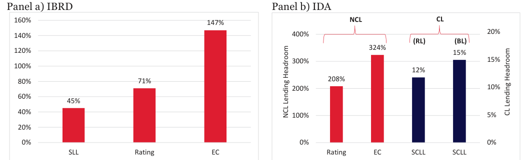
Note: The red bars illustrate, for IBRD and IDA, the headroom for additional non-concessional lending in percent of current net lending and guarantees implied by the three sources of constraint, namely Statutory Lending Limit (indicated by ‘SLL’), the requirement that the AAA-ratings of all three global rating agencies be maintained (labelled ‘Rating’) and that the Capital Adequacy Ratio (equal to capital resources (paid in equity and reserves) divided by capital required (Economic Capital plus a 10% buffer)) exceeds unity. IDA has no SLL constraint. In computing CARs for IDA, we have followed a conservative approach, comparable to IDA’s internal risk management methodology, of adjusting capital resources downwards to allow for the value of the subsidy element in IDA’s loans. More information about the computations may be found in the sister technical paper, Risk Control (2023). The dark blue bars show headroom as a percentage of IDA total lending (relative to the SCLL) if it expands its lending using subsidised loan instruments (CLs or BLs). SCLL denotes Sustainable Concessional Lending Limit, NCL denotes Non-Concessional Loan, CL denotes Concessional Loan, RL denotes Regular Loan and BL denotes Blended Loan. Note that because of the differences in the way these constraints are applied, the rating headroom (71% for IBRD) is expressed in terms of outstanding loans whereas the EC headroom (147% for IBRD) is expressed in terms of outstanding loans plus 50% of undisbursed commitments.
| Blended lending | 26.6 |
|---|---|
| Concessional lending | 21.0 |
| Non-concessional lending | No upper bound |
7.6 Implications of securitisation for lending headroom
Our analysis of the effects of risk transfer on lending headroom are based on the two portfolios described in Section 5. These represent 10% of the EAD of the respective institutions. We assume that the MDB retains the senior and junior tranche while transferring the mezzanine tranche (of thickness 25.25%). We suppose that the retained senior tranche can be rated no higher than single A, applying the Standard & Poor’s approach.
The lending headroom due to securitisation based on credit rating analysis is calculated through a two-step process. First, we calculate the reduction in the adjusted credit RWA after securitisation compared to the same quantity in the base case (see Table 6.4 and Table 6.5). Second, by calculating the percentage increase in the net outstanding loans for the portfolio with securitisation that would lead generate the same adjusted RWAs as in the base case.
Table 7.3 shows the additional amount that the institution could lend following a risk transfer before its Standard & Poor’s RAC ratio equals the value it had before the risk transfer. This additional lending headroom is low for IBRD compared to IDA for similar amount of risk transfer in that, for IBRD the securitisation generates only an additional 3% for portfolio A and 6% for portfolio B, while for IDA it leads to 16% and 13% for the two portfolios. The difference reflects the fact that IBRD makes loans to higher rated countries. The securitisation is less effective in this case. The best outcome for IBRD is the 6% it can achieve with portfolio B.
In Table 7.4, we show the reduction in economic capital (EC) for IBRD and IDA when they securitise their respective portfolios A and B. We find that risk transfer reduces the EC substantially if the securitised portfolio is riskier. for IBRD the reduction in EC is 12% for portfolio A and 18% for portfolio B. For IDA, the reduction in EC turns out to be 12% for both portfolio A and B (see Table 7.4).
These findings imply that risk transfer offers an effective safety valve in relaxing some of the lending constraints that IBRD and IDA may face. But there are some significant obstacles here. For IBRD, the tightest constraint is the SLL. The definition of lending used in calculating the SLL presumably includes retained senior tranches. This severely restricts the benefit that the IBRD might obtain from a risk transfer that leaves a thick senior tranche on balance sheet. If the SLL were relaxed, the first constraint to bind would be the constraint associated with a downgrade in the Moody’s rating. Again, when lending expands, the Moody’s rating is affected by a deterioration in the leverage ratio. This would not be much improved by a risk transfer that left IBRD with a thick retained senior tranche.
| ^ĞĐƵƌŝƚŝƐĂƚŝŽŶ | / Z | / | ||
|---|---|---|---|---|
| ^ĐĞŶĂƌŝŽ | ,ĞĂĚƌŽŽŵ | 'ƌŽƐƐ ǀĂůƵĞ | ,ĞĂĚƌŽŽŵ | 'ƌŽƐƐ ǀĂůƵĞ |
| WŽƌƚĨŽůŝŽ | ϯй | ϲ͕ϯϮϯ | ϭϲй Ϯϳ͕ϳϱϳ | |
| WŽƌƚĨŽůŝŽ | ϲй | ϭϮ͕ϳϱϴ | ϭϯй Ϯϯ͕ϯϵϬ |
Note: Blue shade indicates the portfolio that leads to maximum LH. The % is based on net outstanding loans of respective institutions. The gross value is in $ million.
| ,ĞĂĚƌŽŽŵ ZŝƐŬ ƚƌĂŶƐĨĞƌ ^ĐĞŶĂƌŝŽ | 'ƌŽƐƐ ǀĂůƵĞ ,ĞĂĚƌŽŽŵ | 'ƌŽƐƐ | ǀĂůƵĞ | |
|---|---|---|---|---|
| ZĞĚƵĐƚŝŽŶ | ŝŶ | ZĞĚƵĐƚŝŽŶ ŝŶ ZĞĚƵĐƚŝŽŶ | ŝŶ ZĞĚƵĐƚŝŽŶ | ŝŶ |
| ƌĞƋƵŝƌĞĚ | ƌĞƋƵŝƌĞĚ ƌĞƋƵŝƌĞĚ | ƌĞƋƵŝƌĞĚ | ||
| s Z Ăƚ ϭďƉ ʹ ƌŝƐŬ ƚƌĂŶƐĨĞƌ ŽĨ ƉŽƌƚĨŽůŝŽ | ϭϮй | Ϯ͕ϲϲϵ | ϭϭй | ϯ͕ϭϯϰ |
| s Z Ăƚ ϭďƉ ʹ ƌŝƐŬ ƚƌĂŶƐĨĞƌ ŽĨ ƉŽƌƚĨŽůŝŽ | ϭϴй | ϰ͕Ϭϱϰ | ϭϯй | ϯ͕ϱϭϱ |
Note: Blue shade indicates the portfolio that leads to maximum reduction in EC. The percentage reported is in terms of the base case VAR amount without risk transfer. The gross value is in millions of US dollars.
8. Conclusion
This study examines the constraints on lending faced by the International Bank for Reconstruction and Development (IBRD) and the International Development Association (IDA).
The constraints in question are:
1. The Statutory Lending Limit (SLL) included in the IBRD’s Articles of Agreement. Those of IDA do not include such a limit.
2. The requirement that the two institutions retain their triple A ratings from the three global rating agencies, Moody’s, Standard & Poor’s and Fitch. (IDA is not rated by Fitch.)
3. The requirement that the institutions’ Capital Adequacy Ratios (CARs) exceed unity. The CAR is measured as the ratio of capital resources (typically, the sum of paid in equity, retained earnings and reserves) to capital required (typically measured as the total Economic Capital for different risk types, credit, market and operational).
4. Sustainable Concessional Lending Limit (SCLL) is a limit on total subsidised (zero-interest-rate) lending which cannot exceed its equity if the institution is to sustain this lending over time (for IDA).
We show that for IBRD, the SLL binds first followed by the rating constraint (specifically because of the Moody’s rating, followed by that of Fitch), and that the CAR/Economic Capital limit binds last. IDA is not subject to an SLL. The rating and CAR constraints barely limit how IDA might expand its lending but unless such increased lending were non-concessional, IDA would rapidly hit the Sustainable Concessional Lending Limit (SCLL) in that its total concessional lending (including the concessional component of blended loans) would exceed its equity. This would before long generate losses and a reduction in IDA’s ability to make fully concessional (zero-interest-rate) loans.
Risk transfer appears feasible and could assist in relaxing some constraints. But, for IBRD, the SLL and the constraint associated with Moody’s ratings would not be relaxed by the most standard types of transactions involving tranching since these constraints depend on a combination of the leverage ratio and the contractual support ratio (which depends on callable capital and total debt) which are not sensitive. For IDA, risk transfer is unnecessary since the constraints we examine here are far from binding.
The conclusions of this study are necessarily subject to the assumptions made as part of the analysis. Thus, the precise headroom values that we provide should be treated with caution, but we believe that the broad messages and findings are reliable.
References
Asian Development Bank (2023) “What is IF-CAP? How ADB is Launching a New Era in Climate Finance (ADB Insight Full Episode),” available at: https://www.adb.org/news/videos/what-if-cap-how-adb-launching-newera-climate-finance-adb-insight-full-episode.
Asian Infrastructure Investment Bank (2015) "Articles of Agreement," available at: https://www.aiib.org/en/about-aiib/basic-documents/_download/articles-ofagreement/basic_document_english-bank_articles_of_agreement.pdf.
CAF Panel (2022) “Boosting MDBs’ Investing Capacity - An Independent Review of Multilateral Development Banks’ Capital Adequacy Frameworks,” available at: https://www.dt.mef.gov.it/export/sites/sitodt/modules/documenti_it/news/news/CAF-Review-Report.pdf.
Cruces, Juan J., and Christoph Trebesch (2013) "Sovereign defaults: The price of haircuts," American Economic Journal: Macroeconomics, 5(3), 85-117, available at: https://www.aeaweb.org/articles?id=10.1257/mac.5.3.85
Duponcheele, G., W. Perraudin and D. Totouom-Tangho (2013) “A principles-based approach to regulatory capital for securitisations,” available at: http://www.riskcontrollimited.com/public/Regulatory_capital_for_securitisations.pdf.
European Investment Bank (2020) “Statue and other treaty provisions,” March, available at: https://www.eib.org/attachments/general/statute/eib_statute_2020_03_01_en.pdf.
Fitch Ratings (2023) “Rating Action Commentary – Fitch affirms IBRD at ‘AAA’; Outlook Stable,” January, available at: https://www.fitchratings.com/research/sovereigns/fitch-affirms-ibrd-at-aaa-outlook-stable-20- 01-2023.
Galizia, Federico, William Perraudin, Andrew Powell, and Timothy Turner (2021). “Risk transfer for multilateral development banks: Obstacles and potential,” IDB Working Paper Series, No. IDB-WP-1292, available at: https://publications.iadb.org/en/risk-transfer-multilateral-development-banks-obstacles-andpotential.
Humphrey, Christopher (2017) “Six proposals to strengthen the finances of multilateral development banks,” Overseas Development Institute Working Paper,509, available at: https://www.researchcollection.ethz.ch/bitstream/handle/20.500.11850/130651/2/11451.pdf.
International Bank for Reconstruction and Development and International Development Association (2018) “Management’s Discussion & Analysis and Financial Statements,” June, available at: https://thedocs.worldbank.org/en/doc/474791538065340369-0090022018/original/211296v2.pdf.
International Bank for Reconstruction and Development (2012) “Articles of Agreement,” June, available at: https://thedocs.worldbank.org/en/doc/722361541184234501- 0330022018/original/IBRDArticlesOfAgreementEnglish.pdf.
International Bank for Reconstruction and Development (2020) “Management’s Discussion & Analysis and Financial Statements,” June, available at: https://thedocs.worldbank.org/en/doc/521601597072122154- 0340022020/original/IBRDFinancialStatementsJune2020.pdf.
International Bank for Reconstruction and Development (2021) “Management’s Discussion & Analysis and Financial Statements,” June, available at: https://thedocs.worldbank.org/en/doc/9e6e5c7c885899cba176dd6e1409cbeb-0040012021/original/IBRD- Financial-Statements-June-2021.pdf.
International Bank for Reconstruction and Development (2022) “Management’s Discussion & Analysis and Financial Statements,” June, available at: https://thedocs.worldbank.org/en/doc/16796f0d7a20087d312ec8634ace777c-0040012022/original/IBRD- Financial-Statements-June-2022.pdf.
International Development Association (1960) “Articles of Agreement,” available at: https://thedocs.worldbank.org/en/doc/2a209939e876fdcd0d957036daebff6e-0410011960/original/IDA- Articles-of-Agreement-English.pdf.
International Development Association (2018) “IDA in the capital markets,” available at: https://treasury.worldbank.org/en/about/unit/treasury/ida.
International Development Association (2020) “Management’s Discussion & Analysis and Financial Statements,” June, available at: https://thedocs.worldbank.org/en/doc/716251597072522097- 0340022020/original/IDAFinancialStatementsJune2020.pdf.
International Development Association (2021) “Management’s Discussion & Analysis and Financial Statements,” June, available at: https://thedocs.worldbank.org/en/doc/55ac1406fd9fe61a56e6e5d097ef8251- 0040012021/original/IDA-Financial-Statements-June-2021.pdf.
International Development Association (2022) “Management’s Discussion & Analysis and Financial Statements,” June, available at: https://thedocs.worldbank.org/en/doc/95f18d0acf6cf1aee22f82a82d963da9- 0040012022/original/IDA-Financial-Statements-June-2022.pdf.
International Monetary Fund (2019) “Fiscal Policy and Development: Human, Social, and Physical Investment for the SDGs,” January, available at: https://www.imf.org/- /media/Files/Publications/SDN/2019/SDN1903.ashx.
London School of Economics and Political Science (2022) “Finance for climate actions: Scaling up investment for climate and development,” Grantham Research Institute on Climate Change and the Environment, available at: https://www.lse.ac.uk/granthaminstitute/wp-content/uploads/2022/11/IHLEG-Finance-for-Climate- Action-1.pdf.
Moody’s Investors Service (2023a) “Credit opinion – IBRD (World Bank) – Aaa Stable,” March, available at: https://thedocs.worldbank.org/en/doc/daed9065774b50e10261008f065969ca-0340022023/original/Moodys-IDA-03Feb2023.pdf.
Moody’s Investors Service (2023b) “Credit opinion – International Development Association (IDA) – Aaa Stable,” February, available at: https://thedocs.worldbank.org/en/doc/daed9065774b50e10261008f065969ca- 0340022023/original/Moody-s-IDA-03Feb2023.pdf.
Pykhtin, M. and A. Dev (2002) “Credit risk in asset securitisations: analytical model” Risk, May, pages S16- S20.
Pykhtin, M. (2004) “Asymptotic Model of Economic Capital for Securitisations,” in William Perraudin (ed.), Credit Structured Products, Risk Books.
Risk Control (2019) “Room2Run: the AfDB’s Approach to Sharing Risk with the Private Sector,” April, available at: https://www.riskcontrollimited.com/public/Room-to-Run_Risk-Control.pdf.
Risk Control (2022) “MDB Sovereign Loan Credit Performance and PCT: Public Data Analysis”.
S&P Global Ratings (2018) “Multilateral Lending Institutions Capital Methodology and Assumptions,” 24th October.
S&P Global Ratings (2022a) “Criteria | Governments | General: Multilateral lending institutions and other supranational institutions rating methodology,” January.
S&P Global Ratings (2022b) “Default, Transition, and Recovery: 2021 Annual Global Sovereign Default And Rating Transition Study,” available at: https://www.spglobal.com/ratings/en/research/articles/220504default-transition-and-recovery-2021-annual-global-sovereign-default-and-rating-transition-study-12350530
S&P Global Ratings (2022c) “Ratings Direct – European Investment Bank,” available at: https://www.eib.org/attachments/fi/external/SP_EIB_Report_28Feb2022.pdf.
S&P Global Ratings (2022d) “Supranationals,” October, available at: https://www.spglobal.com/_assets/documents/ratings/research/101567466.pdf.
S&P Global Ratings (2023a) “Ratings Direct – International Bank for Reconstruction and Development,” March, available at: https://thedocs.worldbank.org/en/doc/c8bebad75f48ea4d48815853a7c2c608- 0340022023/original/Final-SP-IBRD-full-report-March-9-2023.pdf.
S&P Global Ratings (2023b) “Ratings Direct – International Development Association,” March, available at: https://thedocs.worldbank.org/en/doc/81046cccaff0f46642555bce13697bc2-0340022023/original/Final-SP- IDA-full-report-March-10-2023.pdf.
Vasicek, Oldrich (1991) “Limiting loan loss probability distribution” mimeo KMV Corporation.
World Bank Group (2018) “World Bank Group Shareholders Endorse Transformative Capital Package,” April, available at: https://www.worldbank.org/en/news/press-release/2018/04/21/world-bank-groupshareholders-endorse-transformative-capital-package.
World Bank Group (2023a) “Evolution of the World Bank Group – A Report to Governors,”30th March, available at: https://www.devcommittee.org/sites/dc/files/download/Documents/2023-03/Final_DC2023- 0002%20evolution%20paper.pdf.
World Bank Repository (2023) “IDA Statement Of Credits and Grants - Historical Data,” 21st June, available at: https://finances.worldbank.org/Loans-and-Credits/IDA-Statement-Of-Credits-and-Grants-Historical- Dat/tdwh-3krx.
Yang, Bill Huajian (2017) “Smoothing Algorithms by Constrained Maximum Likelihood,” June, available at: https://mpra.ub.uni-muenchen.de/79911/1/MPRA_paper_79911.pdf
Appendix 1: Rating Data and Calibration Issues
Standard & Poor’s rating fine-tuning S&P provides an extensive document with a discussion of the factors that are considered for the final rating calculations. This provides detailed descriptions of individual calculations such as the RAC methodology and the liquidity indicators. The exposure at default (EAD) is not explicitly presented in the annual reports from IBRD and IDA. To match the EAD calculated from S&P we apply a factor the net outstanding loans and to the other assets.
The RAC methodology comprises many adjustments to obtain the Total Adjusted Capital (TAC). These adjustments are calculated using the ratings and the correlation matrix of the sovereigns. S&P does not specifically report the date at which the ratings are collected or the period for which correlation matrices, therefore, approximate the adjustments and, thus, ultimately the RAC ratio. We made individual adjustments so as to obtain to the original RAC ratio.
Liquidity indicators are harder to calculate as information is lacking regarding the maturity of the liabilities of IBRD and IDA. By adjusting the maturity of liabilities (we have information on the maturity of the assets), we match the liquidity and funding gap.
Moody’s rating fine-tuning Moody’s have an extensive document on rating methodology. The methodology depends on fewer n quantitative elements than does that of Standard & Poor’s. The leverage ratio (an important determinant on capital adequacy) may be directly inferred from the balance sheet. So, no adjustment was required. The liquidity indicator nonetheless depends on the forecast of inflows and outflows. This forecast is not obtainable from the annual report, so we infer the inflows and outflows so as to match the liquidity factor that appears in the Moody’s report.
We must also infer the answer to the qualitative questions included in the Moody’s methodology. In most cases, we can infer suitable answers to questions based on general knowledge of the institutions. However, some answers are inferred from intermediate indicators reported together with the final rating.
Fitch rating fine-tuning Fitch does not calculate a rating for IDA. Consequently, we lack a reference point to calculate a Fitch rating. Nevertheless, Fitch provides a very extensive discussion of its rating calculation. This specifies some of the quantitative factors that are used to the ratings, but not in a very comprehensive list.
We, therefore, deduce some quantitative calculations from intermediate indicators in the ratings reports. As with the other rating agencies we are obliged to make assumptions regarding the maturity of liabilities to obtain liquidity indicators.
Other adjustments are performed to the answers to qualitative questions to match intermediate ratings results to those that the agency has published.
Appendix 2: Rating Analysis not Changing Qualitative Questions
In this appendix, we display results without answering qualitative questions conservatively. It is more realistic to assume that the agencies would adopt more negative answers to their qualitative questions, but the results show here represent a benchmark against which one may compare the results reported in the main text.
Table A2.1: S&P rating with DRA and treasury growth not qualitative deterioration for IBRD
ZнdƌĞĂƐƵƌLJ &ŝŶĂŶĐŝĂůZŝƐŬ ŶƚĞƌƉƌŝƐĞ ŶŚĂŶĐĞĚ&ŝŶĂŶĐŝĂů ŶŚĂŶĐĞĚ/ŶĚŝĐĂƚŝǀĞ Z;йͿ ϭϮŵŽŶƚŚ &ŝŶĂů/Z ŐƌŽǁƚŚ;йͿ ůŝƋƵŝĚŝƚLJ ĂƉŝƚĂůĚĞƋƵĂĐLJ >ŝƋƵŝĚŝƚLJĂŶĚ&ƵŶĚŝŶŐ WƌŽĨŝůĞ ZŝƐŬWƌŽĨŝůĞ ^W ŶŚĂŶĐĞĚZ;йͿ ZŝƐŬWƌŽĨŝůĞ ^W /Z
Ϭ Ϯϱ͘ϵ ϮϬϬ džƚƌĞŵĞůLJ^ƚƌŽŶŐ džƚƌĞŵĞůLJƐƚƌŽŶŐ ϰϱ͘ϲ ĂĂĂ džƚƌĞŵĞůLJ džƚƌĞŵĞůLJ^ƚƌŽŶŐ ϳϱ ϭϱ͘Ϭ ϭϴϵ͘ϱ sĞƌLJ^ƚƌŽŶŐ sĞƌLJ^ƚƌŽŶŐ Ϯϲ͘ϰ ^ƚƌŽŶŐ ĂĂĂ ĂĂĂ ƐƚƌŽŶŐ ϭϲϰ ϭϬ͘Ϭ ϭϴϯ͘ϳ ^ƚƌŽŶŐ ^ƚƌŽŶŐ ĂĂн ϯϮ͘ϵ
Ϯϳϴ ϳ͘Ϭ ϭϴϬ͘ϰ ĚĞƋƵĂƚĞ ĚĞƋƵĂƚĞ ĂĂ Ϯϴ͘ϲ džƚƌĞŵĞůLJ^ƚƌŽŶŐΎ Note: * These enhanced FRP are held by the qualitative question on the loan performance
Table A2.2: S&P rating with DRA and treasury growth not qualitative deterioration for IDA
ZнdƌĞĂƐƵƌLJ &ŝŶĂŶĐŝĂůZŝƐŬ ŶƚĞƌƉƌŝƐĞ ŶŚĂŶĐĞĚ&ŝŶĂŶĐŝĂů ŶŚĂŶĐĞĚ/ŶĚŝĐĂƚŝǀĞ Z;йͿ ϭϮŵŽŶƚŚ &ŝŶĂů/Z ŐƌŽǁƚŚ;йͿ ůŝƋƵŝĚŝƚLJ ĂƉŝƚĂůĚĞƋƵĂĐLJ >ŝƋƵŝĚŝƚLJĂŶĚ&ƵŶĚŝŶŐ WƌŽĨŝůĞ ZŝƐŬWƌŽĨŝůĞ ^W ŶŚĂŶĐĞĚZ;йͿ ZŝƐŬWƌŽĨŝůĞ ^WΎ /Z
Ϭ ϲϴ͘ϴ ϮϰϬ ^ƚƌŽŶŐ džƚƌĞŵĞůLJƐƚƌŽŶŐ ϲϴ͘ϴ džƚƌĞŵĞůLJƐƚƌŽŶŐ džƚƌĞŵĞůLJ ĂĂĂ ĂĂĂ Ϯϳ ϱϲ ϭϮϲ džƚƌĞŵĞůLJ^ƚƌŽŶŐ ĚĞƋƵĂƚĞ sĞƌLJ^ƚƌŽŶŐ ϱϰ͘ϰ sĞƌLJ^ƚƌŽŶŐ ĂĂĂ ƐƚƌŽŶŐ ϲϰ ϰϰ ϵϬ DŽĚĞƌĂƚĞ ^ƚƌŽŶŐ ĂĂн ϰϯ͘Ϭ ^ƚƌŽŶŐ ĂĂн Note: * There is no change in the enhanced SACP as there is no callable capital for the IDA
Table A2.3: Moody’s rating with DRA and treasury growth not qualitative deterioration for IBRD WƌĞůŝŵŝŶĂƌLJ ŽŶƚƌĂĐƚƵĂů ^ƚƌĞŶŐƚŚŽĨ ZнdƌĞĂƐƵƌLJ >ĞǀĞƌĂŐĞƌĂƚŝŽ ĂƉŝƚĂů >ŝƋƵŝĚŝƚLJĂŶĚ YƵĂůŝƚĂƚŝǀĞ ĚũƵƐƚĞĚŝŶƚƌŝŶƐŝĐ ^ĐŽƌĞĐĂƌĚ ŝŶƚƌŝŶƐŝĐĨŝŶĂŶĐŝĂů ƐƵƉƉŽƌƚƌĂƚŝŽ ŵĞŵďĞƌ ŐƌŽǁƚŚ;йͿ ;йͿ ĂĚĞƋƵĂĐLJ ĨƵŶĚŝŶŐ ĂĚũƵƐƚŵĞŶƚƐ ĨŝŶĂŶĐŝĂůƐƚƌĞŶŐƚŚ /ŶĚŝĐĂƚĞĚ ƐƚƌĞŶŐƚŚ ;йͿ ƐƵƉƉŽƌƚ
Ϭ ϰϱϬ Ăϭ ĂĂϮ ĂĂϭ ϭϮϬ sĞƌLJŚŝŐŚ ϵ ϰϲϴ ĂϮ ϭϭϬ
Table A2.4: Moody’s rating with DRA and treasury growth not qualitative deterioration for IDA
Table A2.5: Fitch rating with DRA and treasury growth not qualitative deterioration for IBRD
Table A2.6: Fitch rating with DRA and treasury growth not qualitative deterioration for IDA
Appendix 3: Calibration of the Capital Model
We explain in this appendix, the assumptions adopted in calibrating the Credit Portfolio Model (CPM) employed in the Capital Adequacy Ratio (CAR) analysis.
Transition matrix We use as starting point the historical transition matrix reported in S&P (2022b). This is based on data up to
2021. The transition matrix is shown in Table A3.5.
We then scale the righthand column to allow for Preferred Creditor Treatment (PCT). Risk Control (2022) has previously analysed the effect of PCT on sovereign PDs. Using historical arrears data from multiple MDBs, it infers a multiplicative adjustment of 1/3.5 to infer PCT-inclusive PDs from those encountered in the sovereign bond market. Table A3.6 shows the PCT adjusted transition matrix we obtain after scaling PDs in this way.
As an alternative approach, we estimate rating-specific PDs inclusive of PCT directly from MDB sovereign loan non-accrual data. This is described in more detail see Appendix 4. The resulting PD vector is inserted in the righthand column of a transition matrix and other row elements rescaled to obtain unity. The resulting matrix is shown in Table A3.7.
Loss Given Default (LGD) We present our results using 4 different sets of LGDs: x Non-stochastic LGDs with PCT adjustments, x Non-stochastic LGDs without PCT adjustments, x Stochastic LGDs with PCT adjustments and x Stochastic LGDs without PCT adjustments.
For the non-stochastic case, we assume that LGDs with PCT adjustments are 10% and LGDs without PCT adjustments are 45%.
For the stochastic case, we suppose that recoveries (equal to unity minus the LGD rate) are beta-distributed on

(2013) estimated mean and standard deviation of haircuts as 37.04 and 27.28 respectively. Using these results,

we calculate the value of ߣ as

adjustments and 55% without PCT adjustments. Therefore, volatilities are 0.168 and 0.279 with and without PCT adjustments respectively.
Correlations Correlation assumptions are crucial inputs to credit portfolio analysis. One common practice is to base correlations on equity return data. Alternatively, one may base correlations on spread changes or rating histories. We, here, consider two approaches based on equity index returns and bond spread changes.
For the equity-index-based approach, we use the regional equity indices that are calculated by MSCI[27]: x MSCI EFM Africa, x MSCI EM Europe and Middle East, x MSCI EM Asia, x MSCI EM Latin America.
Here, EFM stands for Emerging Frontier Markets and EM stands for Emerging Markets. The time-series index data is daily from 02/01/2006 to 14/03/2023. Firstly, we calculate the 6-month overlapping log returns by ݎ[_t] = (ݔ[_t])−(ݔ_{t−182}) where ݔ[_t] is the index value on day ݐ. Then, we normalise the returns by subtracting the mean and dividing by the standard deviation. Finally, we calculate the pairwise correlations between each index. The correlations are displayed in Table A3.1.
Table A3.1: Equity-based Correlation Matrix
ƵƌŽƉĞĂŶĚ >ĂƚŝŶ ĨƌŝĐĂ ƐŝĂ ŽƌƌĞůĂƚŝŽŶ DŝĚĚůĞ ĂƐƚ ŵĞƌŝĐĂ
ĨƌŝĐĂ ϭϬϬ͘ϬϬй ϴϯ͘Ϭϵй ϴϵ͘ϯϲй ϴϵ͘ϲϳй
ƵƌŽƉĞĂŶĚDŝĚĚůĞ ĂƐƚ ϴϯ͘Ϭϵй ϭϬϬ͘ϬϬй ϴϲ͘ϯϭй ϴϱ͘ϱϱй
ƐŝĂ ϴϵ͘ϯϲй ϴϲ͘ϯϭй ϭϬϬ͘ϬϬй ϴϮ͘Ϯϰй
>ĂƚŝŶŵĞƌŝĐĂ ϴϵ͘ϲϳй ϴϱ͘ϱϱй ϴϮ͘Ϯϰй ϭϬϬ͘ϬϬй
To calculate the idiosyncratic risk weights for each region, firstly, we obtain 33 country equity indices that are calculated by MSCI in addition to the region indices and calculate the normalised log returns of the series. We regress the individual country indices on their corresponding region index and obtain the regression coefficient ߚ_i for each country ݅. The reason behind this calculation is the factor model we assumed in equation (4.2). So,
_2. Finally, we

average over each region to calculate the regional idiosyncratic weights. The results appear in Table A3.2.
Table A3.2: Equity-based Idiosyncratic Risk Weights
/ĚŝŽƐLJŶĐƌĂƚŝĐƌŝƐŬ ZĞŐŝŽŶ ǁĞŝŐŚƚƐ;ĞƚĂͿ
Ϭ͘ϳϵϬ ĨƌŝĐĂ
ƵƌŽƉĞĂŶĚDŝĚĚůĞ ĂƐƚ Ϭ͘ϲϱϭ
Ϭ͘ϲϰϱ ƐŝĂ
>ĂƚŝŶŵĞƌŝĐĂ Ϭ͘ϱϵϭ
For the spread-based approach, the data employed consists of corporate bonds covering the universe of publicly offered straight fixed-rate U.S. bonds, a large collection of Eurobonds and government bonds. Our government bond data contains all government sovereign, municipal sovereign and government agency bonds that are issued on major markets (Canada, Eurobond, European Monetary Union, France, Germany, Italy, Japan, UK and US), denominated in US dollar, issuer domicile being non-US and Moody’s rating higher than Caa3. The dataset contains the comprehensive characteristic and price data reported by Refinitiv.
We select the bonds issued by 134 countries that have loans to either IBRD and IDA and group them accordingly into their regions. Regional factor correlations are calculated based on the spread changes of the bonds as described above over the period from 01/02/2006 to 31/10/2022. The following steps are taken to obtain the regional factor correlations:
1. The price of each bond in the database is calculated using information of the bond characteristics (coupon rate, maturity, coupon payment frequency) and is discounted using the zero curve.
2. The default-free yield of each bond is calculated, which represents the internal rate of return such that the sum of the present value of the cash flow is equal to the bond price in 1).
3. The spread for each bond is calculated as the difference between the market yield and the default-free yield.
4. The spread indices are calculated as the difference of the average spreads of commonly existing bonds between two adjacent dates across the entire study period.
5. The regional correlations are then calculated between each pair of regions given the spread indices in 4) as factors.
As the observation period is long, the approach used consists of calculating moments with overlapping observations and then adjusting non-parametrically for the statistical biases induced by the use of overlapping observations. Note that the return correlations vary according to the degree to which the observations are overlapping. We use 250-day as our holding period in this exercise. The correlations are estimated using the steps above are presented in Table A3.3.
Table A3.3: Spread-based Correlation Matrix
ƵƌŽƉĞĂŶĚ >ĂƚŝŶ ĨƌŝĐĂ ƐŝĂ DŝĚĚůĞ ĂƐƚ ŵĞƌŝĐĂ
ĨƌŝĐĂ ϭϬϬ͘ϬϬй ϱϮ͘ϭϰй ϴϬ͘Ϯϯй ϳϮ͘ϰϮй
ƵƌŽƉĞĂŶĚDŝĚĚůĞ ĂƐƚ ϱϮ͘ϭϰй ϭϬϬ͘ϬϬй ϱϭ͘ϲϳй ϱϬ͘Ϭϵй
ƐŝĂ ϴϬ͘Ϯϯй ϱϭ͘ϲϳй ϭϬϬ͘ϬϬй ϲϵ͘ϵϮй
>ĂƚŝŶŵĞƌŝĐĂ ϳϮ͘ϰϮй ϱϬ͘Ϭϵй ϲϵ͘ϵϮй ϭϬϬ͘ϬϬй
We also estimated the idiosyncratic risk weights based on regressions of changes in bond yield spread indices for different regions. The results are given in Table A3.4.
Table A3.4: Spread-based Idiosyncratic Risk Weights /ĚŝŽƐLJŶĐƌĂƚŝĐƌŝƐŬ ZĞŐŝŽŶ ǁĞŝŐŚƚƐ;ĞƚĂͿ
ĨƌŝĐĂ Ϭ͘ϱϲϱ
Ϭ͘ϴϵϰ ƵƌŽƉĞĂŶĚDŝĚĚůĞ ĂƐƚ
Ϭ͘ϳϲϮ ƐŝĂ
>ĂƚŝŶŵĞƌŝĐĂ Ϭ͘ϳϱϵ
Table A3.5: S&P Historical Sovereign Transition Matrix
&ƌŽŵͬdŽ н Ͳ н Ͳ н Ͳ н Ͳ н Ͳ Ɛ ĞĨĂƵůƚ
ϵϲ͘ϳϵй Ϯ͘ϳϭй Ϭ͘ϰϮй Ϭ͘ϬϬй Ϭ͘ϬϬй Ϭ͘ϬϬй Ϭ͘Ϭϭй Ϭ͘ϬϬй Ϭ͘ϬϬй Ϭ͘ϬϬй Ϭ͘ϬϬй Ϭ͘Ϭϳй Ϭ͘ϬϬй Ϭ͘ϬϬй Ϭ͘ϬϬй Ϭ͘ϬϬй Ϭ͘ϬϬй Ϭ͘ϬϬй
н ϲ͘ϰϱй ϴϱ͘ϭϲй ϲ͘ϲϭй ϭ͘ϳϳй Ϭ͘ϬϬй Ϭ͘ϬϬй Ϭ͘ϬϬй Ϭ͘ϬϬй Ϭ͘ϬϬй Ϭ͘ϬϬй Ϭ͘ϬϬй Ϭ͘ϬϬй Ϭ͘ϬϬй Ϭ͘ϬϬй Ϭ͘ϬϬй Ϭ͘ϬϬй Ϭ͘ϬϬй Ϭ͘ϬϬй
Ϭ͘ϬϬй ϲ͘ϮϮй ϴϱ͘ϭϳй ϲ͘ϳϰй Ϭ͘ϱϮй Ϭ͘ϰϮй Ϭ͘ϭϬй Ϭ͘ϱϮй Ϭ͘ϬϬй Ϭ͘ϬϬй Ϭ͘ϬϬй Ϭ͘ϯϭй Ϭ͘ϬϬй Ϭ͘ϬϬй Ϭ͘ϬϬй Ϭ͘ϬϬй Ϭ͘ϬϬй Ϭ͘ϬϬй
Ͳ Ϭ͘ϬϬй Ϭ͘ϬϬй ϳ͘ϴϮй ϴϯ͘ϰϱй ϳ͘ϭϲй Ϭ͘ϭϳй Ϭ͘ϱϬй Ϭ͘ϭϳй Ϭ͘ϬϬй Ϭ͘ϭϳй Ϭ͘ϰϰй Ϭ͘ϬϬй Ϭ͘ϬϬй Ϭ͘ϭϭй Ϭ͘ϬϬй Ϭ͘ϬϬй Ϭ͘ϬϬй Ϭ͘ϬϬй
н Ϭ͘ϬϬй Ϭ͘ϬϬй Ϭ͘Ϭϳй ϭϯ͘ϯϱй ϳϯ͘Ϯϴй ϵ͘ϯϬй Ϯ͘Ϭϯй ϭ͘ϭϮй Ϭ͘ϭϰй Ϭ͘ϲϯй Ϭ͘Ϭϳй Ϭ͘ϬϬй Ϭ͘ϬϬй Ϭ͘ϬϬй Ϭ͘ϬϬй Ϭ͘ϬϬй Ϭ͘ϬϬй Ϭ͘Ϭϭй
Ϭ͘ϬϬй Ϭ͘ϬϬй Ϭ͘ϬϬй ϭ͘ϭϱй ϭϮ͘ϯϯй ϳϳ͘Ϯϵй ϱ͘ϳϭй ϭ͘ϲϴй Ϭ͘ϳϳй Ϭ͘ϵϲй Ϭ͘ϭϬй Ϭ͘ϬϬй Ϭ͘ϬϬй Ϭ͘ϬϬй Ϭ͘ϬϬй Ϭ͘ϬϬй Ϭ͘ϬϬй Ϭ͘Ϭϭй
Ͳ Ϭ͘ϬϬй Ϭ͘ϬϬй Ϭ͘ϬϬй Ϭ͘ϬϬй Ϭ͘ϵϰй ϭϭ͘ϰϳй ϳϳ͘ϴϮй ϲ͘ϵϰй Ϭ͘ϰϭй ϭ͘ϱϳй Ϭ͘ϲϳй Ϭ͘ϭϲй Ϭ͘ϬϬй Ϭ͘ϬϬй Ϭ͘ϬϬй Ϭ͘ϬϬй Ϭ͘ϬϬй Ϭ͘ϬϮй
н Ϭ͘ϬϬй Ϭ͘ϬϬй Ϭ͘ϬϬй Ϭ͘ϬϬй Ϭ͘ϬϬй Ϯ͘ϭϲй ϭϮ͘ϯϵй ϳϬ͘ϴϲй ϭϭ͘Ϯϰй Ϯ͘ϰϭй Ϭ͘ϲϬй Ϭ͘Ϯϰй Ϭ͘Ϭϲй Ϭ͘ϬϬй Ϭ͘ϬϬй Ϭ͘ϬϬй Ϭ͘ϬϬй Ϭ͘Ϭϰй
Ϭ͘ϬϬй Ϭ͘ϬϬй Ϭ͘ϬϬй Ϭ͘ϬϬй Ϭ͘ϬϬй Ϭ͘ϬϬй ϭ͘ϴϳй ϭϲ͘ϲϬй ϲϴ͘Ϭϱй ϭϭ͘ϭϲй Ϭ͘ϵϵй Ϭ͘ϭϭй Ϭ͘ϬϬй Ϭ͘ϱϬй Ϭ͘ϮϮй Ϭ͘ϭϭй Ϭ͘ϯϯй Ϭ͘Ϭϲй
Ͳ Ϭ͘ϬϬй Ϭ͘ϬϬй Ϭ͘ϬϬй Ϭ͘ϬϬй Ϭ͘ϬϬй Ϭ͘ϬϬй Ϭ͘ϬϬй Ϭ͘ϵϯй ϭϰ͘ϵϰй ϳϰ͘ϲϵй ϲ͘ϱϬй Ϯ͘ϭϯй Ϭ͘Ϯϳй Ϭ͘Ϭϴй Ϭ͘ϭϱй Ϭ͘ϭϮй Ϭ͘Ϭϴй Ϭ͘ϭϭй
н Ϭ͘ϬϬй Ϭ͘ϬϬй Ϭ͘ϬϬй Ϭ͘ϬϬй Ϭ͘ϬϬй Ϭ͘ϬϬй Ϭ͘ϬϬй Ϭ͘ϬϬй Ϭ͘ϱϰй ϮϬ͘ϱϳй ϲϲ͘ϯϴй ϵ͘ϵϯй ϭ͘ϭϰй Ϭ͘ϭϴй Ϭ͘Ϭϲй Ϭ͘ϬϬй ϭ͘ϬϮй Ϭ͘ϭϴй
Ϭ͘ϬϬй Ϭ͘ϬϬй Ϭ͘ϬϬй Ϭ͘ϬϬй Ϭ͘ϬϬй Ϭ͘ϬϬй Ϭ͘ϬϬй Ϭ͘ϬϬй Ϭ͘ϬϬй Ϭ͘ϳϴй ϭϰ͘ϮϬй ϳϬ͘ϴϬй ϭϭ͘ϭϱй ϭ͘ϴϬй Ϭ͘ϲϴй Ϭ͘ϭϱй Ϭ͘Ϭϱй Ϭ͘ϰϬй
Ͳ Ϭ͘ϬϬй Ϭ͘ϬϬй Ϭ͘ϬϬй Ϭ͘ϬϬй Ϭ͘ϬϬй Ϭ͘ϬϬй Ϭ͘ϬϬй Ϭ͘ϬϬй Ϭ͘ϬϬй Ϭ͘ϬϬй ϭ͘Ϭϯй ϭϬ͘ϱϱй ϳϯ͘ϳϵй ϭϭ͘ϰϳй ϭ͘ϭϵй Ϭ͘ϰϲй Ϭ͘ϲϭй Ϭ͘ϵϬй
н Ϭ͘ϬϬй Ϭ͘ϬϬй Ϭ͘ϬϬй Ϭ͘ϬϬй Ϭ͘ϬϬй Ϭ͘ϬϬй Ϭ͘ϬϬй Ϭ͘ϬϬй Ϭ͘ϬϬй Ϭ͘Ϭϯй Ϭ͘Ϭϯй Ϭ͘ϵϮй ϭϬ͘ϮϬй ϲϴ͘ϳϬй ϭϱ͘ϯϬй Ϯ͘ϱϬй Ϭ͘ϴϱй ϭ͘ϰϲй
Ϭ͘ϬϬй Ϭ͘ϬϬй Ϭ͘ϬϬй Ϭ͘ϬϬй Ϭ͘ϬϬй Ϭ͘ϬϬй Ϭ͘ϬϬй Ϭ͘ϬϬй Ϭ͘ϬϬй Ϭ͘ϬϬй Ϭ͘ϬϬй Ϭ͘ϬϬй Ϭ͘ϲϭй ϭϯ͘ϱϬй ϳϬ͘ϳϳй ϵ͘ϴϰй Ϯ͘ϵϭй Ϯ͘ϯϴй
Ͳ Ϭ͘ϬϬй Ϭ͘ϬϬй Ϭ͘ϬϬй Ϭ͘ϬϬй Ϭ͘ϬϬй Ϭ͘ϬϬй Ϭ͘ϬϬй Ϭ͘ϬϬй Ϭ͘ϬϬй Ϭ͘ϬϬй Ϭ͘ϬϬй Ϭ͘ϬϬй Ϭ͘ϬϬй Ϯ͘ϰϯй ϭϱ͘Ϭϳй ϲϲ͘ϴϱй ϴ͘Ϭϱй ϳ͘ϱϵй
Ɛ Ϭ͘ϬϬй Ϭ͘ϬϬй Ϭ͘ϬϬй Ϭ͘ϬϬй Ϭ͘ϬϬй Ϭ͘ϬϬй Ϭ͘ϬϬй Ϭ͘ϬϬй Ϭ͘ϬϬй Ϭ͘ϬϬй Ϭ͘ϬϬй Ϭ͘ϬϬй Ϭ͘ϬϬй Ϭ͘ϳϰй ϭ͘ϴϭй ϭϯ͘ϵϬй ϯϮ͘Ϭϴй ϱϭ͘ϰϳй
ĞĨĂƵůƚ Ϭ͘ϬϬй Ϭ͘ϬϬй Ϭ͘ϬϬй Ϭ͘ϬϬй Ϭ͘ϬϬй Ϭ͘ϬϬй Ϭ͘ϬϬй Ϭ͘ϬϬй Ϭ͘ϬϬй Ϭ͘ϬϬй Ϭ͘ϬϬй Ϭ͘ϬϬй Ϭ͘ϬϬй Ϭ͘ϬϬй Ϭ͘ϬϬй Ϭ͘ϬϬй Ϭ͘ϬϬй ϭϬϬ͘ϬϬй Note: Estimates are based on S&P (2022b).
Table A3.6: Historical Sovereign Transition Matrix with Adjusted PDs
&ƌŽŵͬdŽ н Ͳ н Ͳ н Ͳ н Ͳ н Ͳ Ɛ ĞĨĂƵůƚ
ϵϲ͘ϳϵй Ϯ͘ϳϭй Ϭ͘ϰϮй Ϭ͘ϬϬй Ϭ͘ϬϬй Ϭ͘ϬϬй Ϭ͘Ϭϭй Ϭ͘ϬϬй Ϭ͘ϬϬй Ϭ͘ϬϬй Ϭ͘ϬϬй Ϭ͘Ϭϳй Ϭ͘ϬϬй Ϭ͘ϬϬй Ϭ͘ϬϬй Ϭ͘ϬϬй Ϭ͘ϬϬй Ϭ͘ϬϬй
н ϲ͘ϰϱй ϴϱ͘ϭϲй ϲ͘ϲϭй ϭ͘ϳϳй Ϭ͘ϬϬй Ϭ͘ϬϬй Ϭ͘ϬϬй Ϭ͘ϬϬй Ϭ͘ϬϬй Ϭ͘ϬϬй Ϭ͘ϬϬй Ϭ͘ϬϬй Ϭ͘ϬϬй Ϭ͘ϬϬй Ϭ͘ϬϬй Ϭ͘ϬϬй Ϭ͘ϬϬй Ϭ͘ϬϬй
Ϭ͘ϬϬй ϲ͘ϮϮй ϴϱ͘ϭϳй ϲ͘ϳϰй Ϭ͘ϱϮй Ϭ͘ϰϮй Ϭ͘ϭϬй Ϭ͘ϱϮй Ϭ͘ϬϬй Ϭ͘ϬϬй Ϭ͘ϬϬй Ϭ͘ϯϭй Ϭ͘ϬϬй Ϭ͘ϬϬй Ϭ͘ϬϬй Ϭ͘ϬϬй Ϭ͘ϬϬй Ϭ͘ϬϬй
Ͳ Ϭ͘ϬϬй Ϭ͘ϬϬй ϳ͘ϴϮй ϴϯ͘ϰϱй ϳ͘ϭϲй Ϭ͘ϭϳй Ϭ͘ϱϬй Ϭ͘ϭϳй Ϭ͘ϬϬй Ϭ͘ϭϳй Ϭ͘ϰϰй Ϭ͘ϬϬй Ϭ͘ϬϬй Ϭ͘ϭϭй Ϭ͘ϬϬй Ϭ͘ϬϬй Ϭ͘ϬϬй Ϭ͘ϬϬй
н Ϭ͘ϬϬй Ϭ͘ϬϬй Ϭ͘Ϭϳй ϭϯ͘ϯϱй ϳϯ͘Ϯϴй ϵ͘ϯϬй Ϯ͘Ϭϯй ϭ͘ϭϮй Ϭ͘ϭϰй Ϭ͘ϲϯй Ϭ͘Ϭϳй Ϭ͘ϬϬй Ϭ͘ϬϬй Ϭ͘ϬϬй Ϭ͘ϬϬй Ϭ͘ϬϬй Ϭ͘ϬϬй Ϭ͘ϬϬй
Ϭ͘ϬϬй Ϭ͘ϬϬй Ϭ͘ϬϬй ϭ͘ϭϱй ϭϮ͘ϯϯй ϳϳ͘ϯϬй ϱ͘ϳϭй ϭ͘ϲϴй Ϭ͘ϳϳй Ϭ͘ϵϲй Ϭ͘ϭϬй Ϭ͘ϬϬй Ϭ͘ϬϬй Ϭ͘ϬϬй Ϭ͘ϬϬй Ϭ͘ϬϬй Ϭ͘ϬϬй Ϭ͘ϬϬй
Ͳ Ϭ͘ϬϬй Ϭ͘ϬϬй Ϭ͘ϬϬй Ϭ͘ϬϬй Ϭ͘ϵϰй ϭϭ͘ϰϳй ϳϳ͘ϴϯй ϲ͘ϵϰй Ϭ͘ϰϭй ϭ͘ϱϳй Ϭ͘ϲϳй Ϭ͘ϭϲй Ϭ͘ϬϬй Ϭ͘ϬϬй Ϭ͘ϬϬй Ϭ͘ϬϬй Ϭ͘ϬϬй Ϭ͘Ϭϭй
н Ϭ͘ϬϬй Ϭ͘ϬϬй Ϭ͘ϬϬй Ϭ͘ϬϬй Ϭ͘ϬϬй Ϯ͘ϭϲй ϭϮ͘ϰϬй ϳϬ͘ϴϳй ϭϭ͘Ϯϱй Ϯ͘ϰϭй Ϭ͘ϲϬй Ϭ͘Ϯϰй Ϭ͘Ϭϲй Ϭ͘ϬϬй Ϭ͘ϬϬй Ϭ͘ϬϬй Ϭ͘ϬϬй Ϭ͘Ϭϭй
Ϭ͘ϬϬй Ϭ͘ϬϬй Ϭ͘ϬϬй Ϭ͘ϬϬй Ϭ͘ϬϬй Ϭ͘ϬϬй ϭ͘ϴϳй ϭϲ͘ϲϭй ϲϴ͘Ϭϴй ϭϭ͘ϭϳй Ϭ͘ϵϵй Ϭ͘ϭϭй Ϭ͘ϬϬй Ϭ͘ϱϬй Ϭ͘ϮϮй Ϭ͘ϭϭй Ϭ͘ϯϯй Ϭ͘ϬϮй
Ͳ Ϭ͘ϬϬй Ϭ͘ϬϬй Ϭ͘ϬϬй Ϭ͘ϬϬй Ϭ͘ϬϬй Ϭ͘ϬϬй Ϭ͘ϬϬй Ϭ͘ϵϯй ϭϰ͘ϵϱй ϳϰ͘ϳϱй ϲ͘ϱϭй Ϯ͘ϭϯй Ϭ͘Ϯϳй Ϭ͘Ϭϴй Ϭ͘ϭϱй Ϭ͘ϭϮй Ϭ͘Ϭϴй Ϭ͘Ϭϯй
н Ϭ͘ϬϬй Ϭ͘ϬϬй Ϭ͘ϬϬй Ϭ͘ϬϬй Ϭ͘ϬϬй Ϭ͘ϬϬй Ϭ͘ϬϬй Ϭ͘ϬϬй Ϭ͘ϱϰй ϮϬ͘ϱϵй ϲϲ͘ϰϳй ϵ͘ϵϰй ϭ͘ϭϰй Ϭ͘ϭϴй Ϭ͘Ϭϲй Ϭ͘ϬϬй ϭ͘ϬϮй Ϭ͘Ϭϱй
Ϭ͘ϬϬй Ϭ͘ϬϬй Ϭ͘ϬϬй Ϭ͘ϬϬй Ϭ͘ϬϬй Ϭ͘ϬϬй Ϭ͘ϬϬй Ϭ͘ϬϬй Ϭ͘ϬϬй Ϭ͘ϳϴй ϭϰ͘Ϯϰй ϳϭ͘Ϭϭй ϭϭ͘ϭϴй ϭ͘ϴϬй Ϭ͘ϲϴй Ϭ͘ϭϱй Ϭ͘Ϭϱй Ϭ͘ϭϮй
Ͳ Ϭ͘ϬϬй Ϭ͘ϬϬй Ϭ͘ϬϬй Ϭ͘ϬϬй Ϭ͘ϬϬй Ϭ͘ϬϬй Ϭ͘ϬϬй Ϭ͘ϬϬй Ϭ͘ϬϬй Ϭ͘ϬϬй ϭ͘Ϭϰй ϭϬ͘ϲϮй ϳϰ͘Ϯϳй ϭϭ͘ϱϰй ϭ͘ϮϬй Ϭ͘ϰϲй Ϭ͘ϲϭй Ϭ͘Ϯϲй
н Ϭ͘ϬϬй Ϭ͘ϬϬй Ϭ͘ϬϬй Ϭ͘ϬϬй Ϭ͘ϬϬй Ϭ͘ϬϬй Ϭ͘ϬϬй Ϭ͘ϬϬй Ϭ͘ϬϬй Ϭ͘Ϭϯй Ϭ͘Ϭϯй Ϭ͘ϵϯй ϭϬ͘ϯϭй ϲϵ͘ϰϯй ϭϱ͘ϰϲй Ϯ͘ϱϮй Ϭ͘ϴϲй Ϭ͘ϰϮй
Ϭ͘ϬϬй Ϭ͘ϬϬй Ϭ͘ϬϬй Ϭ͘ϬϬй Ϭ͘ϬϬй Ϭ͘ϬϬй Ϭ͘ϬϬй Ϭ͘ϬϬй Ϭ͘ϬϬй Ϭ͘ϬϬй Ϭ͘ϬϬй Ϭ͘ϬϬй Ϭ͘ϲϮй ϭϯ͘ϳϯй ϳϮ͘ϬϬй ϭϬ͘Ϭϭй Ϯ͘ϵϲй Ϭ͘ϲϴй
Ͳ Ϭ͘ϬϬй Ϭ͘ϬϬй Ϭ͘ϬϬй Ϭ͘ϬϬй Ϭ͘ϬϬй Ϭ͘ϬϬй Ϭ͘ϬϬй Ϭ͘ϬϬй Ϭ͘ϬϬй Ϭ͘ϬϬй Ϭ͘ϬϬй Ϭ͘ϬϬй Ϭ͘ϬϬй Ϯ͘ϱϴй ϭϱ͘ϵϲй ϳϬ͘ϳϴй ϴ͘ϱϮй Ϯ͘ϭϳй
Ɛ Ϭ͘ϬϬй Ϭ͘ϬϬй Ϭ͘ϬϬй Ϭ͘ϬϬй Ϭ͘ϬϬй Ϭ͘ϬϬй Ϭ͘ϬϬй Ϭ͘ϬϬй Ϭ͘ϬϬй Ϭ͘ϬϬй Ϭ͘ϬϬй Ϭ͘ϬϬй Ϭ͘ϬϬй ϭ͘ϯϭй ϯ͘ϭϵй Ϯϰ͘ϰϮй ϱϲ͘ϯϴй ϭϰ͘ϳϬй
ĞĨĂƵůƚ Ϭ͘ϬϬй Ϭ͘ϬϬй Ϭ͘ϬϬй Ϭ͘ϬϬй Ϭ͘ϬϬй Ϭ͘ϬϬй Ϭ͘ϬϬй Ϭ͘ϬϬй Ϭ͘ϬϬй Ϭ͘ϬϬй Ϭ͘ϬϬй Ϭ͘ϬϬй Ϭ͘ϬϬй Ϭ͘ϬϬй Ϭ͘ϬϬй Ϭ͘ϬϬй Ϭ͘ϬϬй ϭϬϬ͘ϬϬй Note: Estimates are based on S&P (2022b).
Table A3.7: Historical Non-accrual Transition Matrix
&ƌŽŵͬdŽ н Ͳ н Ͳ н Ͳ н Ͳ н Ͳ Ɛ ĞĨĂƵůƚ
ϵϲ͘ϳϵй Ϯ͘ϳϭй Ϭ͘ϰϮй Ϭ͘ϬϬй Ϭ͘ϬϬй Ϭ͘ϬϬй Ϭ͘Ϭϭй Ϭ͘ϬϬй Ϭ͘ϬϬй Ϭ͘ϬϬй Ϭ͘ϬϬй Ϭ͘Ϭϳй Ϭ͘ϬϬй Ϭ͘ϬϬй Ϭ͘ϬϬй Ϭ͘ϬϬй Ϭ͘ϬϬй Ϭ͘ϬϬй
н ϲ͘ϰϱй ϴϱ͘ϭϲй ϲ͘ϲϭй ϭ͘ϳϳй Ϭ͘ϬϬй Ϭ͘ϬϬй Ϭ͘ϬϬй Ϭ͘ϬϬй Ϭ͘ϬϬй Ϭ͘ϬϬй Ϭ͘ϬϬй Ϭ͘ϬϬй Ϭ͘ϬϬй Ϭ͘ϬϬй Ϭ͘ϬϬй Ϭ͘ϬϬй Ϭ͘ϬϬй Ϭ͘ϬϬй
Ϭ͘ϬϬй ϲ͘ϮϮй ϴϱ͘ϭϳй ϲ͘ϳϰй Ϭ͘ϱϮй Ϭ͘ϰϮй Ϭ͘ϭϬй Ϭ͘ϱϮй Ϭ͘ϬϬй Ϭ͘ϬϬй Ϭ͘ϬϬй Ϭ͘ϯϭй Ϭ͘ϬϬй Ϭ͘ϬϬй Ϭ͘ϬϬй Ϭ͘ϬϬй Ϭ͘ϬϬй Ϭ͘ϬϬй
Ͳ Ϭ͘ϬϬй Ϭ͘ϬϬй ϳ͘ϴϮй ϴϯ͘ϰϱй ϳ͘ϭϲй Ϭ͘ϭϳй Ϭ͘ϱϬй Ϭ͘ϭϳй Ϭ͘ϬϬй Ϭ͘ϭϳй Ϭ͘ϰϰй Ϭ͘ϬϬй Ϭ͘ϬϬй Ϭ͘ϭϭй Ϭ͘ϬϬй Ϭ͘ϬϬй Ϭ͘ϬϬй Ϭ͘ϬϬй
н Ϭ͘ϬϬй Ϭ͘ϬϬй Ϭ͘Ϭϳй ϭϯ͘ϯϱй ϳϯ͘Ϯϴй ϵ͘ϯϬй Ϯ͘Ϭϯй ϭ͘ϭϮй Ϭ͘ϭϰй Ϭ͘ϲϯй Ϭ͘Ϭϳй Ϭ͘ϬϬй Ϭ͘ϬϬй Ϭ͘ϬϬй Ϭ͘ϬϬй Ϭ͘ϬϬй Ϭ͘ϬϬй Ϭ͘Ϭϭй
Ϭ͘ϬϬй Ϭ͘ϬϬй Ϭ͘ϬϬй ϭ͘ϭϱй ϭϮ͘ϯϯй ϳϳ͘Ϯϵй ϱ͘ϳϭй ϭ͘ϲϴй Ϭ͘ϳϳй Ϭ͘ϵϲй Ϭ͘ϭϬй Ϭ͘ϬϬй Ϭ͘ϬϬй Ϭ͘ϬϬй Ϭ͘ϬϬй Ϭ͘ϬϬй Ϭ͘ϬϬй Ϭ͘Ϭϭй
Ͳ Ϭ͘ϬϬй Ϭ͘ϬϬй Ϭ͘ϬϬй Ϭ͘ϬϬй Ϭ͘ϵϰй ϭϭ͘ϰϳй ϳϳ͘ϴϮй ϲ͘ϵϰй Ϭ͘ϰϭй ϭ͘ϱϳй Ϭ͘ϲϳй Ϭ͘ϭϲй Ϭ͘ϬϬй Ϭ͘ϬϬй Ϭ͘ϬϬй Ϭ͘ϬϬй Ϭ͘ϬϬй Ϭ͘ϬϮй
н Ϭ͘ϬϬй Ϭ͘ϬϬй Ϭ͘ϬϬй Ϭ͘ϬϬй Ϭ͘ϬϬй Ϯ͘ϭϲй ϭϮ͘ϯϵй ϳϬ͘ϴϲй ϭϭ͘Ϯϰй Ϯ͘ϰϭй Ϭ͘ϲϬй Ϭ͘Ϯϰй Ϭ͘Ϭϲй Ϭ͘ϬϬй Ϭ͘ϬϬй Ϭ͘ϬϬй Ϭ͘ϬϬй Ϭ͘Ϭϯй
Ϭ͘ϬϬй Ϭ͘ϬϬй Ϭ͘ϬϬй Ϭ͘ϬϬй Ϭ͘ϬϬй Ϭ͘ϬϬй ϭ͘ϴϳй ϭϲ͘ϲϬй ϲϴ͘Ϭϲй ϭϭ͘ϭϲй Ϭ͘ϵϵй Ϭ͘ϭϭй Ϭ͘ϬϬй Ϭ͘ϱϬй Ϭ͘ϮϮй Ϭ͘ϭϭй Ϭ͘ϯϯй Ϭ͘Ϭϱй
Ͳ Ϭ͘ϬϬй Ϭ͘ϬϬй Ϭ͘ϬϬй Ϭ͘ϬϬй Ϭ͘ϬϬй Ϭ͘ϬϬй Ϭ͘ϬϬй Ϭ͘ϵϯй ϭϰ͘ϵϱй ϳϰ͘ϳϮй ϲ͘ϱϬй Ϯ͘ϭϯй Ϭ͘Ϯϳй Ϭ͘Ϭϴй Ϭ͘ϭϱй Ϭ͘ϭϮй Ϭ͘Ϭϴй Ϭ͘Ϭϳй
н Ϭ͘ϬϬй Ϭ͘ϬϬй Ϭ͘ϬϬй Ϭ͘ϬϬй Ϭ͘ϬϬй Ϭ͘ϬϬй Ϭ͘ϬϬй Ϭ͘ϬϬй Ϭ͘ϱϰй ϮϬ͘ϱϴй ϲϲ͘ϰϰй ϵ͘ϵϰй ϭ͘ϭϰй Ϭ͘ϭϴй Ϭ͘Ϭϲй Ϭ͘ϬϬй ϭ͘ϬϮй Ϭ͘ϭϬй
Ϭ͘ϬϬй Ϭ͘ϬϬй Ϭ͘ϬϬй Ϭ͘ϬϬй Ϭ͘ϬϬй Ϭ͘ϬϬй Ϭ͘ϬϬй Ϭ͘ϬϬй Ϭ͘ϬϬй Ϭ͘ϳϴй ϭϰ͘Ϯϰй ϳϬ͘ϵϵй ϭϭ͘ϭϳй ϭ͘ϴϬй Ϭ͘ϲϴй Ϭ͘ϭϱй Ϭ͘Ϭϱй Ϭ͘ϭϰй
Ͳ Ϭ͘ϬϬй Ϭ͘ϬϬй Ϭ͘ϬϬй Ϭ͘ϬϬй Ϭ͘ϬϬй Ϭ͘ϬϬй Ϭ͘ϬϬй Ϭ͘ϬϬй Ϭ͘ϬϬй Ϭ͘ϬϬй ϭ͘Ϭϰй ϭϬ͘ϲϯй ϳϰ͘ϯϮй ϭϭ͘ϱϱй ϭ͘ϮϬй Ϭ͘ϰϲй Ϭ͘ϲϭй Ϭ͘ϭϵй
н Ϭ͘ϬϬй Ϭ͘ϬϬй Ϭ͘ϬϬй Ϭ͘ϬϬй Ϭ͘ϬϬй Ϭ͘ϬϬй Ϭ͘ϬϬй Ϭ͘ϬϬй Ϭ͘ϬϬй Ϭ͘Ϭϯй Ϭ͘Ϭϯй Ϭ͘ϵϯй ϭϬ͘ϯϯй ϲϵ͘ϱϭй ϭϱ͘ϰϴй Ϯ͘ϱϯй Ϭ͘ϴϲй Ϭ͘Ϯϵй
Ϭ͘ϬϬй Ϭ͘ϬϬй Ϭ͘ϬϬй Ϭ͘ϬϬй Ϭ͘ϬϬй Ϭ͘ϬϬй Ϭ͘ϬϬй Ϭ͘ϬϬй Ϭ͘ϬϬй Ϭ͘ϬϬй Ϭ͘ϬϬй Ϭ͘ϬϬй Ϭ͘ϲϮй ϭϯ͘ϳϲй ϳϮ͘ϭϱй ϭϬ͘Ϭϯй Ϯ͘ϵϳй Ϭ͘ϰϳй
Ͳ Ϭ͘ϬϬй Ϭ͘ϬϬй Ϭ͘ϬϬй Ϭ͘ϬϬй Ϭ͘ϬϬй Ϭ͘ϬϬй Ϭ͘ϬϬй Ϭ͘ϬϬй Ϭ͘ϬϬй Ϭ͘ϬϬй Ϭ͘ϬϬй Ϭ͘ϬϬй Ϭ͘ϬϬй Ϯ͘ϲϭй ϭϲ͘ϭϴй ϳϭ͘ϳϳй ϴ͘ϲϰй Ϭ͘ϳϵй
Ɛ Ϭ͘ϬϬй Ϭ͘ϬϬй Ϭ͘ϬϬй Ϭ͘ϬϬй Ϭ͘ϬϬй Ϭ͘ϬϬй Ϭ͘ϬϬй Ϭ͘ϬϬй Ϭ͘ϬϬй Ϭ͘ϬϬй Ϭ͘ϬϬй Ϭ͘ϬϬй Ϭ͘ϬϬй ϭ͘ϰϵй ϯ͘ϲϯй Ϯϳ͘ϴϰй ϲϰ͘Ϯϲй Ϯ͘ϳϳй
ĞĨĂƵůƚ Ϭ͘ϬϬй Ϭ͘ϬϬй Ϭ͘ϬϬй Ϭ͘ϬϬй Ϭ͘ϬϬй Ϭ͘ϬϬй Ϭ͘ϬϬй Ϭ͘ϬϬй Ϭ͘ϬϬй Ϭ͘ϬϬй Ϭ͘ϬϬй Ϭ͘ϬϬй Ϭ͘ϬϬй Ϭ͘ϬϬй Ϭ͘ϬϬй Ϭ͘ϬϬй Ϭ͘ϬϬй ϭϬϬ͘ϬϬй
One way to understand the conservativeness or otherwise of the calibrated correlations is to compute the pairwise correlation of the latent variables driving any two exposures. If one averages across all pairs of exposures in a portfolio, the resulting mean pairwise latent variable correlation may be compared to the correlations assumed in the Basel rules. In the Basel Internal Ratings Based Approach (IRBA), capital is calculated assuming that any loans have latent variable correlations ranging from 12% to 24% depending on the credit quality as measured by the probability of default. Computing pairwise asset correlations for the IBRD and IDA portfolios, we obtain the following results: Equity-based IBRD average pairwise correlation: 49.33% Equity-based IDA average pairwise correlation: 44.12% Spread-based IBRD average pairwise correlation: 30.16% Spread-based IDA average pairwise correlation: 40.60% This suggests that the calibration we consider are distinctly more conservative than is assumed in Basel.
Appendix 4: Sensitivity Analysis of PDs
Sovereign Probability of Default (PD) is a key parameter in the capital calculation employed in assessment of portfolio credit risk. This appendix explains how we estimate PDs using the non-accrual data from four prominent MDBs, namely Asian Development Bank (ADB), International Bank for Reconstruction and Development (IBRD), Inter-American Development Bank (IDB) and African Development Bank (AfDB).
Use of S&P sovereign historical PDs is inappropriate for MDBs as they omit the important influence of Preferred Creditor Treatment (PCT). In our calculation, a sovereign is counted as being in default when it is placed into non-accrual status by at least one of the Multinational Development Banks (MDBs) that reports an outstanding balance for that sovereign. We employ data for the time period 1988-2019. A total of 48 nonaccrual events may be found in the dataset considered.
The key inputs for the sovereign PD model are historical non-accrual (default) data from ADB, IADB, IBRD and AfDB and the historical S&P ratings of the sovereigns. Information on the data is presented in Table A4.1and Table A4.2. Some non-accrual events for AfDB and IADB are shared with IBRD since the latter has borrower countries in common with ADB, AfDB, and IADB. In the final data used for the calculation, the shared member countries are excluded from the IBRD dataset to avoid double counting.
Table A4.1: Countries Count in the Historical Non-accrual Data
ηEŽŶͲĐĐƌƵĂů /ŶƐƚŝƚƵƚŝŽŶ ^ŽƵƌĐĞ ηŽƵŶƚƌŝĞƐ ŽƵŶƚƌŝĞƐ /ŶƚĞƌŶĂů ϰϳ ϳ Ĩ ŶŶƵĂůZĞƉŽƌƚƐ ϱϮ ϭϮ / / Ϯϰ ϳ /Z ŶŶƵĂůZĞƉŽƌƚƐ ϭϲϮ ϮϮ dŽƚĂů Ϯϴϱ ϰϴ
Table A4.2: Non-accrual Countries
ƌĞĚŝƚŽƌ &ŝƌƐƚEŽŶͲĐĐƌƵĂů ƌĞĚŝƚŽƌ &ŝƌƐƚEŽŶͲ /ŶƐƚŝƚƵƚŝŽŶ ^ŽǀĞƌĞŝŐŶ zĞĂƌ /ŶƐƚŝƚƵƚŝŽŶ ^ŽǀĞƌĞŝŐŶ ĐĐƌƵĂůzĞĂƌ ĨŐŚĂŶŝƐƚĂŶ ϭϵϵϯ /Z ŽƐŶŝĂĂŶĚ,ĞƌnjĞŐŽǀŝŶĂ ϭϵϵϯ DĂƌƐŚĂůů/ƐůĂŶĚƐ ϮϬϬϲ /Z ,Ăŝƚŝ ϭϵϵϮ͕ϮϬϬϮ DLJĂŶŵĂƌ ϭϵϵϴ /Z /ƌĂƋ ϭϵϵϭ EĂƵƌƵ ϮϬϬϭ /Z DŽŶƚĞŶĞŐƌŽ ϭϵϵϳ ^ŽůŽŵŽŶ/ƐůĂŶĚƐ ϭϵϵϲ͕ϮϬϬϯ /Z EŽƌƚŚDĂĐĞĚŽŶŝĂ ϭϵϵϯ
sŝĞƚŶĂŵ ϭϵϵϮ /Z ^ĞƌďŝĂ ϭϵϵϳ DŝĐƌŽŶĞƐŝĂ ϮϬϬϵ /Z ^LJƌŝĂ ϭϵϴϴ͕ϮϬϭϮ Ĩ ĂďŽsĞƌĚĞ ϮϬϭϳ / ĂƌďĂĚŽƐ ϮϬϭϮ Ĩ ĞŶƚƌĂůĨƌŝĐĂŶZĞƉƵďůŝĐ ϭϵϵϴ͕ϮϬϬϮ / ŽůŽŵďŝĂ ϮϬϬϯ Ĩ ŽŵŽƌŽƐ ϭϵϵϵ͕ϮϬϬϰ / ŽŵŝŶŝĐĂŶZĞƉƵďůŝĐ ϮϬϬϳ Ĩͬ/Z ƀƚĞĚΖ/ǀŽŝƌĞ ϮϬϬϭ͕ϮϬϬϰ /ͬ/Z 'ƵĂƚĞŵĂůĂ ϭϵϵϭ Ĩͬ/Z ĞŵŽĐƌĂƚŝĐZĞƉƵďůŝĐŽĨƚŚĞŽŶŐŽ ϭϵϵϰ͕ϮϬϬϰ /ͬ/Z 'ƵLJĂŶĂ ϭϵϴϴ Ĩ ũŝďŽƵƚŝ ϮϬϬϱ /ͬ/Z ,ŽŶĚƵƌĂƐ ϭϵϴϵ Ĩ ƌŝƚƌĞĂ ϮϬϭϮ /ͬ/Z EŝĐĂƌĂŐƵĂ ϭϵϴϴ Ĩ 'ƵŝŶĞĂ ϮϬϭϬ /ͬ/Z WĂŶĂŵĂ ϭϵϴϴ͕ϮϬϬϮ Ĩͬ/Z >ŝďĞƌŝĂ ϭϵϴϴ /ͬ/Z WĞƌƵ ϭϵϴϴ Ĩͬ/Z ZĞƉƵďůŝĐŽĨŽŶŐŽ ϭϵϵϮ͕ϭϵϵϴ͕ϮϬϬϰ / ^ƵƌŝŶĂŵĞ ϮϬϬϬ Ĩ ^ĞŶĞŐĂů ϮϬϭϳ / dƌŝŶŝĚĂĚĂŶĚdŽďĂŐŽ ϭϵϵϵ Ĩͬ/Z ^ĞLJĐŚĞůůĞƐ ϮϬϬϯ / sĞŶĞnjƵĞůĂ ϮϬϭϳ Ĩͬ/Z ^ŝĞƌƌĂ>ĞŽŶĞ ϭϵϴϴ Ĩ ^ŽŵĂůŝĂ ϭϵϵϮ Ĩͬ/Z ^ƵĚĂŶ ϭϵϵϰ Ĩ dŽŐŽ ϮϬϬϮ Ĩͬ/Z ĂŵďŝĂ ϭϵϴϴ Ĩͬ/Z ŝŵďĂďǁĞ ϮϬϬϭ
IBRD has experienced 22 non-accrual events while the numbers for ADB and IADB are much lower at 7. IADB reports the highest number of non-accrual events per borrowing country. IBRD reports the lowest number of non-accruals per borrowing country. Table A4.2 provides more detailed information on the non-accrual countries for each of the four MDBs.
For each sovereign in the non-accrual data, there is a historical outstanding balance record. A non-accrual event is only treated as a default if at least one MDB has an outstanding balance for that sovereign in the same time period. The non-accrual events of Nauru in 2001 and Democratic Republic of the Congo in 1994 are not counted in this respect as there was no outstanding balance data in the corresponding period in either case. All other non-accrual events are counted as defaults.
The historical sovereign ratings data includes 182 countries and covers time period from 1987 to 2020. The CCC, CC and C ratings by S&P is consolidated to ‘Cs’ in the capital model used in this study. Some sovereigns were not rated (NR) during the earlier periods in the data. The number of NR entries in each year is shown in Table A4.3.
There are 21 non-accruals/defaults that are NR were independently rated by RMPA – Country Ratings Desk using ADB’s Sovereign Rating methodology. The new ratings for these NR entries are shown in Table A4.4
The other NR entries are filled depend on whether there is an existing rating either in previous years or in following years. A two steps approach is adopted to fill in the NR entries. o Step 1: For each country, starting from ݐ_1 and work forward to ݐ_2ǡ ݐ_3ǡ ǥ ǡ ݐ_T, if ݐ_i is NR replace it with the rating at ݐ_{i−1}. ܶ is the total number of time periods. o Step 2: For each country, starting from ݐ_T and work backward to ݐ_{T−1}ǡ ǥ ǡ ݐ_2ǡ ݐ_1, if ݐ_i is NR replace it with the rating at ݐ_{i+1}
Table A4.3: Number of rated and NR countries
zĞĂƌ ZĂƚĞĚ EZ zĞĂƌ ZĂƚĞĚ EZ
ϭϵϴϳ ϭϬ ϭϳϮ ϮϬϬϰ ϭϱϰ Ϯϴ
ϭϵϴϴ ϭϴ ϭϲϰ ϮϬϬϱ ϭϱϰ Ϯϴ
ϭϵϴϵ ϮϬ ϭϲϮ ϮϬϬϲ ϭϱϯ Ϯϵ
ϭϵϵϬ Ϯϯ ϭϱϵ ϮϬϬϳ ϭϱϱ Ϯϳ
ϭϵϵϭ Ϯϳ ϭϱϱ ϮϬϬϴ ϭϱϲ Ϯϲ
ϭϵϵϮ Ϯϰ ϭϱϴ ϮϬϬϵ ϭϲϵ ϭϯ
ϭϵϵϯ ϯϬ ϭϱϮ ϮϬϭϬ ϭϲϵ ϭϯ
ϭϵϵϰ ϯϰ ϭϰϴ ϮϬϭϭ ϭϳϭ ϭϭ
ϭϵϵϱ ϰϬ ϭϰϮ ϮϬϭϮ ϭϳϭ ϭϭ
ϭϵϵϲ ϱϲ ϭϮϲ ϮϬϭϯ ϭϳϯ ϵ
ϭϵϵϳ ϳϬ ϭϭϮ ϮϬϭϰ ϭϳϰ ϴ
ϭϵϵϴ ϳϲ ϭϬϲ ϮϬϭϱ ϭϳϰ ϴ
ϭϵϵϵ ϭϰϰ ϯϴ ϮϬϭϲ ϭϳϰ ϴ
ϮϬϬϬ ϭϱϬ ϯϮ ϮϬϭϳ ϭϳϰ ϴ
ϮϬϬϭ ϭϱϬ ϯϮ ϮϬϭϴ ϭϳϳ ϱ
ϮϬϬϮ ϭϱϭ ϯϭ ϮϬϭϵ ϭϳϳ ϱ
ϮϬϬϯ ϭϱϮ ϯϬ ϮϬϮϬ ϭϳϳ ϱ
To make use of all the available data, assumptions are made to replace the NR entries with proxy ratings.
Table A4.4: New ratings for NR non-accrual
ƌĞĚŝƚŽƌ ĞĨĂƵůƚ ZĞƉůĂĐĞEZ /ŶƐƚŝƚƵƚŝŽŶ ŽƵŶƚƌLJ LJĞĂƌ EZLJĞĂƌ ǁŝƚŚƌĂƚŝŶŐ
ĨŐŚĂŶŝƐƚĂŶ ϭϵϴϵ ϭϵϴϴ н
ϭϵϵϮ ϭϵϵϭ
DĂƌƐŚĂůů/ƐůĂŶĚƐ ϮϬϬϲ ϮϬϬϱ н
DŝĐƌŽŶĞƐŝĂ ϮϬϬϵ ϮϬϬϴ Ͳ
DLJĂŶŵĂƌ ϭϵϵϴ ϭϵϵϳ
^ŽůŽŵŽŶ/ƐůĂŶĚƐ ϭϵϵϲ ϭϵϵϱ Ͳ
sŝĞƚŶĂŵ ϭϵϵϮ ϭϵϵϭ н
Ĩ ĞŶƚƌĂůĨƌŝĐĂŶZĞƉƵďůŝĐ ϭϵϵϴ ϭϵϵϳ н
Ĩ ŽŵŽƌŽƐ ϭϵϵϵ ϭϵϵϴ
ϮϬϬϰ ϮϬϬϯ н
Ĩ ũŝďŽƵƚŝ ϮϬϬϱ ϮϬϬϰ
Ĩ ZĞƉƵďůŝĐŽĨŽŶŐŽ ϭϵϵϮ ϭϵϵϭ
ϭϵϵϴ ϭϵϵϳ
Ĩ ^ŽŵĂůŝĂ ϭϵϵϮ ϭϵϵϭ
Ĩ ^ƵĚĂŶ ϭϵϵϰ ϭϵϵϯ
/Z ,Ăŝƚŝ ϭϵϵϮ ϭϵϵϭ н
/Z /ƌĂƋ ϭϵϵϭ ϭϵϵϬ
/Z DŽŶƚĞŶĞŐƌŽ ϭϵϵϳ ϭϵϵϲ Ͳ
/Z ^ĞƌďŝĂ ϭϵϵϳ ϭϵϵϲ Ͳ
/ 'ƵĂƚĞŵĂůĂ ϭϵϵϭ ϭϵϵϬ Ͳ
/ ,ŽŶĚƵƌĂƐ ϭϵϴϵ ϭϵϴϴ
Based on the historical ratings, non-accrual and outstanding balance data, a table of rating transition and non-

accrual status is constructed. The value in each period is in format of
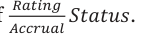
In each year ݐ, the 1-year Rating/Accrual Status is constructed as follows.

ݎܽݐ݅݊݃݅݊ݕ݁ܽݎݐ−ͳǡ ݐ݄݁ݎݓ݅ݏ݁ ͳǡ ݊݊ܽܿܿݎݑ݈ܽ=ͳ ݅݊ݕ݁ܽݎݐܽ݊݀ݑݐݏݐܾ݈ܽ݊݀݅݊݃ܽܽ݊ܿ݁=ͳ ݅݊ݕ݁ܽݎݐ−ͳ (A3.1)

ܰܣǡ ݑݐݏݐܾ݈ܽ݊݀݅݊݃ܽܽ݊ܿ݁=Ͳ ݅݊ݕ݁ܽݎݐ−ͳ
Table A4.5 shows some examples of Rating/Accrual Status for Afghanistan.
Table A4.5: Afghanistan rating/accrual status table
ϭϵϴϴ ϭϵϴϵ ϭϵϵϬ ϭϵϵϭ ϭϵϵϮ ϭϵϵϯ ϭϵϵϰϮϬϬϬ ϮϬϬϭ ϮϬϬϮ ϮϬϬϯ ϮϬϬϰ ϮϬϬϱ ϮϬϬϲͲϮϬϭϳ ϮϬϭϴ ϮϬϭϵ
ZĂƚŝŶŐ ϭϳ ϭϳ ϭϳ ϭϴ ϭϴ ϭϴ ϭϴ ϭϵ ϭϵ ϭϵ ϭϵ ϭϵ ϭϵ ϭϵ ϭϵ
EŽŶͲĂĐĐƌƵĂů ϭ ϭ ϭ ϭ ϭ ϭ
KƵƚƐƚĂŶĚŝŶŐďĂůĂŶĐĞ ϭ ϭ ϭ ϭ ϭ ϭ ϭ ϭ ϭ ϭ Ϭ Ϭ Ϭ ϭ ϭ
ϭͲLJĞĂƌZĂƚŝŶŐͬĐĐƵƌĂů
^ƚĂƚƵƐ ϭϳͬϭ ϮϯͬϬ ϭϳͬϬ ϭϴͬϭ Ϯϯͬϭ Ϯϯͬϭ Ϯϯͬϭ Ϯϯͬϭ ϮϯͬϬ ϭϵͬϬ ϭϵͬE ϭϵͬE ϭϵͬE ϭϵͬϬ Note: The first three rows show the input historical data. The last row displays the rating transition and accrual status for 1year transition.
A table containing all 173 sovereigns is created for the 1-year transitions accordingly. The rows represent countries and columns represent time periods. From the Rating/Accrual Status table, the marginal default rate (MDR) for each rating grade is calculated by counting the number of defaults and total number of obligors. The 1-year MDRs for rating grade ݅ are calculated as follows:
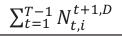
(A3.2)

_{t+1}ǡ_D is the total number of ݅-rated sovereigns at ݐ and with first non-accrual at ݐ+ͳ. Only the obligors with

outstanding balance will be counted. In another word, it is the total number of all _1 entries in the ͳ-year

Rating/Accrual Status table in year ݐ. All _{NA} entries are discarded.
A well-behaved default probability curve should satisfy two important properties: x Default probabilities should be monotonically increasing as credit quality decreases. x Default probabilities should be non-zero.
The raw PDs displayed in Table A4.6 do not possess the above two properties. To produce a well-behaved default probability curve, the raw PDs must be smoothed so that the PDs are monotonic and non-zero.
Thus, the PD curve is smoothened using the logistic form of the PD and the parameters ߙ and ߚ are calculated by using the Maximum Likelihood (ML) method proposed by Yang (2017). The paragraphs below summarize the practical implementation of the method:
Under the monotonic assumption for PD curve, the PD for rating grade ݔ is assumed to take the following logistic form:

ܲܦ[_x](ߙǡ ߚ)≈

Table A4.6: Marginal Default Rates EŽŶͲ EŽŶͲ
&ŝŶĞ &ƌŽŵͬ ĞĨĂ ĞĨĂ &ŝŶĞ &ƌŽŵͬ ĞĨĂ ĞĨĂ
ZĂƚŝŶŐƐ dŽ Ƶůƚ Ƶůƚ DZ ZĂƚŝŶŐƐ dŽ Ƶůƚ Ƶůƚ DZ
Ϭ Ϯ Ϭ͘ϬϬй ϭ ϮϯϮ Ϭ͘ϰϯй
н н Ϭ Ϭ E Ͳ Ͳ Ϭ Ϯϰϭ Ϭ͘ϬϬй
Ϭ ϭϮ Ϭ͘ϬϬй н н ϭ ϯϵϬ Ϭ͘Ϯϲй
Ͳ Ͳ Ϭ ϯϬ Ϭ͘ϬϬй ϰ ϯϳϰ ϭ͘Ϭϲй
н н Ϭ Ϯϴ Ϭ͘ϬϬй Ͳ Ͳ ϲ ϰϰϰ ϭ͘ϯϯй
Ϭ ϲϭ Ϭ͘ϬϬй Ϭ ϭϴ
Ͳ Ͳ Ϭ ϭϯϴ Ϭ͘ϬϬй Ϭ ϲ
Ɛ Ϯ͘ϯϳй н н Ϭ ϵϵ Ϭ͘ϬϬй Ͳ ϭϯ ϵϮϱ
Ϭ ϭϰϲ Ϭ͘ϬϬй ϵ ϱϯ
Ͳ Ͳ ϭ Ϯϭϴ Ϭ͘ϰϲй н ϲ ϭϱϬ
н н Ϯ ϭϳϱ ϭ͘ϭϯй
Here, x ܰ denotes non-default,
![Equation: _x σ_{j=1Nj} x ܨ_N(ݔ)=[ܺ≤ݔȁܰ]= σ_{Jj=1Nj}, _j _j](/api/media/file/eq-273-300x33.png?prefix=media)
x ܰ_j is the total number of ݆-rated sovereigns (total number of _0 and _1 entries in the Rating/Accrual Status table), and

survival into another distribution that is approximately normal even if the distribution is not continuous.
In the discontinuous case, ܨ_N(ݔ) may be equal to 1. ܨ_N(ݔ) is replaced by an average to avoid it is being equal to 1.

(A3.4)

Let ܦ_i and ܰ_i denote the number of defaults and the number of observations for a rating ݅ . Let ܲܦ_i(ߙǡ ߚ) denote MDR, ܲܦ_i(ߙǡ ߚ) is calculated as in equation (A3.3). We assume that the default frequency follows a binomial distribution. Then we can express the log likelihood of the default/non-default sample by:

One may solve for ߙ and ߚ by maximizing the log likelihood function.
Substituting the ݅-year default/non-default count data into equation (A3.5) and maximizing the likelihood function we can obtain ߙ and ߚ estimates for each sample count data. From the estimated ߙ and ߚ parameter and the corresponding count data we can calculate the ͳ-year MDRs using equation (A3.3).
The Maximum Likelihood (ML) approach yields high PDs for the high credit end (results not presented in the report). The parameters in the ML approach are solved by maximizing the loglikelihood function. In this case, one can impose a constraint to force the PDs at the high credit quality end of the curve to be lower in value.
Thus, the constraints are placed for rating AAA and AA estimated PDs such that it is always equal to or lower than the corresponding S&P’s PDs. The estimated parameters based on CML are ߙ equal to 5.443 and ߚ equal to 1.865.
In Table, we can see the smoothened PDs which follows the two properties of a well-behaved default probability curve and the estimated PDs for higher credit rating is of comparable value with the S&P PDs. We compare the S&P PDs and the estimated PDs to obtain the magnitude of the PCT for historical default data of the MDBs.
Table A4.7: Smoothed PDs and Comparison with S&P PD &ŝŶĞ ƐƚŝŵĂƚĞĚ &ŝŶĞ ƐƚŝŵĂƚĞĚ
ZĂƚŝŶŐƐ ^ΘWWƐ WƐ ZĂƚŝŽ ZĂƚŝŶŐƐ ^ΘWWƐ WƐ ZĂƚŝŽ
Ϭ͘ϬϬϭй Ϭ͘ϬϬϭй ϭ͘ϰϴ Ͳ Ϭ͘ϭϬϳй Ϭ͘ϬϳϬй ϭ͘ϱϮ
н Ϭ͘ϬϬϮй Ϭ͘ϬϬϭй ϭ͘ϳϱ н Ϭ͘ϭϴϬй Ϭ͘ϭϬϭй ϭ͘ϳϵ
Ϭ͘ϬϬϯй Ϭ͘ϬϬϮй ϭ͘ϯϲ Ϭ͘ϰϬϯй Ϭ͘ϭϯϵй Ϯ͘ϴϵ
Ͳ Ϭ͘ϬϬϱй Ϭ͘ϬϬϱй ϭ͘Ϭϭ Ͳ Ϭ͘ϵϬϭй Ϭ͘ϭϵϰй ϰ͘ϲϯ
н Ϭ͘ϬϬϴй Ϭ͘ϬϬϴй ϭ͘Ϭϰ н ϭ͘ϰϲϯй Ϭ͘Ϯϵϯй ϰ͘ϵϵ
Ϭ͘Ϭϭϯй Ϭ͘ϬϭϮй ϭ͘ϭϮ Ϯ͘ϯϳϳй Ϭ͘ϰϳϮй ϱ͘Ϭϰ
Ͳ Ϭ͘ϬϮϯй Ϭ͘ϬϮϭй ϭ͘Ϭϲ Ͳ ϳ͘ϱϵϯй Ϭ͘ϳϵϮй ϵ͘ϱϴ
н Ϭ͘Ϭϯϴй Ϭ͘Ϭϯϯй ϭ͘ϭϰ Ɛ ϱϭ͘ϰϲϲй Ϯ͘ϳϳϱй ϭϴ͘ϱϱ
Ϭ͘Ϭϲϰй Ϭ͘Ϭϰϳй ϭ͘ϯϲ ǀĞƌĂŐĞ ϯ͘ϱϱ Note: Ratio is between S&P PDs to the Estimated PDs.
We get an average of 3.55 across the Fine Ratings which is similar to the value of 3.5 which was used to scale down the S&P PDs to adjust for the PCT. It is interesting to note that for the lower rating values B and Cs which historically most of the default sovereigns are rated, the average ratio is 9.54 which is almost three the time the whole sample average ratio. Thus, using the value of 3.5 to scale down the PDs might be considered conservative based on the above analysis.
Appendix 5: Portfolio Loss Rate Calculation
This appendix explains how to calculate the PLR.
i) Compute the unexpected loss (UL) corresponding to a given rating ݅:
ܷܮ=ܴܹܣ×ͺΨ (A5.1)
where the RWA is the Risk Weighted Assets according to S&P’s RAC Framework.
ii) Compute the three-year normalized expected loss (EL) for sovereign exposures. First, the one-year normalized expected loss is calculated as follows:

Here, the ܮܴ_{SOV} is one-year normalized loss rate which depends on the ratings of the sovereigns.
Then the three-year normalized expected loss is three times the one-year normalized expected loss.
(A5.3) ܧܮ_3 =͵ ×ܧܮ_1
iii) Compute the total loss (TL) as, (A5.4) ܶܮ=ܷܮ+ܧܮ_3
iv) This gives the portfolio loss rate (PLR) as:
ܶܮ ܲܮܴ= ܶݐ݈ܽܧܣܦ (A5.5)
Table A3.1: S&P’s Normalized Loss Rates for Sovereigns ZĂƚŝŶŐ E>Z ZĂƚŝŶŐ E>Z ZĂƚŝŶŐ E>Z ZĂƚŝŶŐ E>Z ZĂƚŝŶŐ E>Z
;ďƉƐͿ ;ďƉƐͿ ;ďƉƐͿ ;ďƉƐͿ ;ďƉƐͿ
Ϭ ϳ н ϱϰ Ͳ ϭϵϵ ^ ϯϲϬ
н Ϭ Ͳ ϭϭ ϳϯ н Ϯϰϱ ϯϲϬ
ϭ н ϭϴ Ͳ ϵϳ Ϯϵϵ
Ͳ Ϯ Ϯϳ н ϭϮϱ Ͳ ϯϲϬ
н ϰ Ͳ ϯϵ ϭϱϵ ϯϲϬ
Appendix 6: Tranche rating using the S&P RACF
In this subsection, we implement an approach to infer the rating of the retained tranche from the S&P Risk Adjusted Capital (RAC) framework. This approach, permitted by S&P, was devised by S&P for rating the senior tranche in the Room2Run deal, and is described briefly in Standard & Poor’s (2018). The approach involves, in effect, treating the reference portfolio as a mini-MDB, calculating the threshold level at which such an MDB might issue debt while still retaining a single A rating (where the rating is based on only parts of the RAC approach).
It would be straightforward to generalize this “mini-MDB” approach to obtain a set of loss thresholds corresponding to ratings other than single A. But S&P has so far only endorsed this approach for inferring a single A rating. For the moment, therefore, an MDB may only achieve a single-A rating for a retained senior tranche using this method.
How does the approach work? It involves calculating a stressed level of losses, based on the pool Adjusted RACF RWAs multiplied by 8%, plus an adjustment for Expected Losses (Els). The stressed loss adjusted for Els is referred to under the RACF methodology as the Portfolio Loss Rate (PLR). If the protection provided by more junior tranches exceeds the PLR level of losses, S&P assigns a single A rating to the senior tranche.
This mini-MDB approach devised by S&P to assign an A rating is extended by calculating the Unexpected Losses (ULs) based on 15% and 23% for AA and AAA respectively. We have taken the lower limit for the “very strong” and “extremely strong” from Table A6.1 as the threshold value to be multiplied for stress level AA and AAA respectively.
Table A6.1: Initial Capital Adequacy Assessment ƐƐĞƐƐŵĞŶƚ ZZĂƚŝŽ ƐƐĞƐƐŵĞŶƚ ZZĂƚŝŽ džƚƌĞŵĞůLJ^ƚƌŽŶŐ ϮϯйĂŶĚĂďŽǀĞ DŽĚĞƌĂƚĞ &ƌŽŵϱйƚŽůĞƐƐƚŚĂŶϳй sĞƌLJ^ƚƌŽŶŐ &ƌŽŵϭϱйƚŽůĞƐƐƚŚĂŶϮϯй tĞĂŬ &ƌŽŵϯйƚŽůĞƐƐƚŚĂŶϱй ^ƚƌŽŶŐ &ƌŽŵϭϬйƚŽůĞƐƐƚŚĂŶϭϱй sĞƌLJtĞĂŬ >ĞƐƐƚŚĂŶϯй ĚĞƋƵĂƚĞ &ƌŽŵϳйƚŽůĞƐƐƚŚĂŶϭϬй
Table A6.2: Portfolio Loss Rate
The methodology used for the calculation of the EL and PLR is provided in Appendix 1. The PLRs of all four reference portfolios for the senior tranche are lower than the attachment point as seen in Table A6.2. The attachment point is on average more than double the PLR for stress level A. Thus, the protection provided by the mezzanine tranches is more than the PLR for a single A stress event.
This approach assigns a rating of single A to all four reference portfolios, namely IBRD A, IBRD B, IDA A, and IDA B. Furthermore, using the extended approach all four portfolios could be assigned an AA rating, and only portfolio IBRD A could be assigned an AAA rating.
Appendix 7: Tranche Pricing
Consider a perfectly granular portfolio with total par value normalised to equal unity made up of homogeneous 1-period loans. Suppose that a given loan in the portfolio (with subscript i) defaults if a normally distributed latent variable, ܼ_i , falls below a threshold, −ܿ where ܲܦ = ܰ(−ܿ) is the probability of default for each homogeneous loan. We may express the latent variable for the ith loan as follows:
(A7.1)

Here, ܻ is a common factor, ߳_i is an idiosyncratic shock and both ܻ and ߳_i are standard normal random variables. Appendix 1 of Duponcheele et al (2013) shows that the Expected Loss (EL) on a tranche attaching at ܣ and detaching at ܦ equals.


ͳ −ܺ (A7.2)

In the above equation, ܧܮ̴ܵ݁݊݅ݎ(ܺ) equals the expected loss for a senior tranche with attachment point ܺ and ܰ2(, , ) is the bivariate cumulative standard normal distribution function. This formula is well-known in the literature. It resembles expressions in Pykhtin and Dev (2002) and Pykhtin (2004) which, in turn, build on the work of Vasicek (1991).
The inputs we need for the above calculation are the pool exposure probability of default and Loss Given Default denoted PD and LGD, and the correlation parameter ߩ_{pool}. If we know the Expected Loss on the pool, ܧܮ_{pool}, and the pool loan LGD, we can infer ܲܦ = ܧܮ_{pool}/ܮܩܦ and write equation (A7.2) with inputs ܧܮ_{pool} and LGD.
The above yields Expected Losses for a thick tranche in terms of pool Expected Losses ܧܮ_{pool}, loan Loss Given Default, LGD, and loan correlation ߩ_{pool}. Both pool and tranche Expected Losses here are under historical distributions, i.e., they correspond to Expected Losses as used, for example, by rating agencies or accountants calculating provisions.
As is well known in pricing theory, one may derive the values of prices in a frictionless market by calculating expected, discounted payoffs using risk-adjusted distributions. It is important to note that the results expressed in equations (A7.1) and (A7.2) remain correct if one replaces the actual PDs with risk-adjusted probabilities of default. (We will assume here that loss rates given default are constant and hence not subject to riskadjustment.)
Hence, (A7.1) and (A7.2) represent pricing expressions that may be used to deduce risk-adjusted expected losses for a provider of tranche protection to the pool. To calculate the risk-adjusted expected loss using these equations, requires the inputs of risk-adjusted PD, an LGD rate and a pool correlation parameter. Consider a _R , that pool of credit exposures (bonds or loans) with a given rating R. Suppose we observe the market spread, ܵ_τ investors require to hold these exposures. The risk-adjusted Expected Loss, ܧܮ_{Riskadjusted}, for such loans with an EAD of 1 unit may be calculated as:
(A7.3)

Here, ߬ is the maturity of the loans. ܧܮ_{Riskadjusted} may be thought of as the discount in value of the defaultable loans because of credit risk. If the loans have a constant ܮܩܦ, we can infer from this a risk adjusted probability of default using
(A7.4)

ܮܩܦ
Note that the LGD one uses to infer ܲܦܴ݅ݏ݆݇ܽ݀ݑݏݐ݁݀ should be that appropriate to the instruments in question. For example, if spreads are taken from bond markets, one may presume that the LGD is similar to that commonly observed in historical bond market data such as 50% for senior unsecured bonds.
In contrast, the LGD that we employ in evaluating the expression ܧܮ_{Tℎick}(ܣǡ ܦ) should then be appropriate to the pool of loans under consideration which may well be lower. Given a value for the correlation parameter ߩ_{pool}, we can infer a tranche spread using:
(A7.5)

Note that equation (A7.5) just inverts the relationship between risk adjusted Expected Losses and spread employed in (A7.3) and applies it for the exposure tranche rather than for the pool loans.
To employ the methodology described above, we need to infer a risk adjusted EL for the pool. To do this, we will scale up the historical or actual PD using a scaling factor inferred from the public bond market for which we can deduce actual PDs and risk adjusted PDs from Credit Default Swap (CDS) spreads.
For the latter spreads, we employ the mid-spread data of the senior unsecured Sovereign Credit Default Swap (CDS) for a five-year term instrument. The PDs from the mid spread data are using (5.1) and assuming constant Loss Given Default as 0.55 which is the industry standard for such instruments.
(A7.6) ܲܦ= ܯ݅݀ݏݎ݁ܽ݀ ܮܩܦ
Here mid spread is equivalent to the expected losses of the instrument for a risk-adjusted return instrument. The Scale Factor (SF) is the ratio between PDs of the CDS and five-year S&P’s sovereign PDs which are adjusted for PCT. The scale factor for Aaa and Aa is adjusted by incorporating an intercept of 35 basis points (the lower PDs of Aaa and Aa. The SF was adjusted to have a floor value of 1.
Table A7.1: Scale Factor for PDs using CDS
Thus, from the above exercise, we could scale the five-year S&P Sovereign PDs by relevant SF based on the rating of the sovereign. The pooled portfolio parameters are calculated for various scenarios considered with a constant LGD of 10% seen in Table 6.8.
The pooled correlation ߩ_{pool} of the portfolio is calculated by taking the average of the correlation of individual exposure and the portfolio. Let ߩ_i be the correlation between exposure ݅ and the portfolio and ߟ_i be the equity based idiosyncratic weight (see Table A3.2), and ߩ_{ij} be the equity-based correlation coefficient (see Table A3.1) then:

ܰ
The pricing of the tranche based on expected loss is evaluated using the unscaled 5-Yr PDs which are adjusted for the PCT. The pricing of the tranche with a risk premium is calculated by taking the scaled 5-Yr PDs using the mid-spread data of the CDS. There is third scenario considered to commensurate with the market expectations of the tranching pricing which could be achieved by scaling the pooled PD by a factor of 2, this scenario is thus treated as using conservative PDs.
Appendix 8: S&P Historical Ratings
In this subsection, we analyse the sovereign ratings movements during severe financial crises affecting multiple countries. We consider three crises: (i) the Asian Financial Crisis (1997), (ii) Global Financial Crisis (GFC)
(2008) and (iii) the COVID-19 crisis (2020). The data used in the analysis are summarised in Table A8.1.
We consider, in each case, panel data for sovereign ratings for a five-year window centred on the primary crisis year. Any sovereigns for which data are missing or that is not rated during the crisis period is dropped. The data is collected from the Bloomberg terminal and consists of the sovereign rating on 1st January each year. The S&P ratings are converted to a numeric scale of 1-22. Here, AAA corresponds to 1 and D corresponds to 22. An average of the rating change of sovereigns between year ݐ and ݐ−ͳ is calculated for a given year ݐ. The Average Rating Shift column in Table A8.1 is based on the worst credit downgrades of the sovereign during the crisis.
Table A8.1: Summary of Sovereign Rating Data ^ĐĞŶĂƌŝŽ zĞĂƌƐ ηŽĨŽƵŶƚƌŝĞƐ ǀĞƌĂŐĞZĂƚŝŶŐ^ŚŝĨƚ
ƐŝĂŶ&ŝŶĂŶĐŝĂůƌŝƐŝƐ ϭϵϵϱͲϵϵ ϰϳ Ϭ͘ϯϰ
'& ϮϬϬϲͲϭϬ ϭϬϭ Ϭ͘ϭϴ
Ks/Ͳϭϵ ϮϬϭϵͲϮϯ ϭϭϰ Ϭ͘ϭϮ
Note: The source is Bloomberg.
In Table A8.2 and Table A8.3, the countries that experienced rating changes during the COVID-19 crisis and the worst of GFC and COVID-19 are presented. The tables show downgrades as positive (so upgrades are measured as negative numbers). As shown in Table A8.2, in the COVID-19 crisis, 19 countries experienced downgrades in this period. Note that Argentina was upgraded by 3 notches in this period. Table A8.3 shows that a total of 27 countries experienced downgrades when the worse rating changes in the GFC and COVID-19 periods are combined.
Table A8.2: List of Countries Notched for COVID-19 ŽǁŶͲ ŽǁŶͲ ŽǁŶͲ ŽǁŶͲ ŽƵŶƚƌLJ ŐƌĂĚĞ ŽƵŶƚƌLJ ŐƌĂĚĞ ŽƵŶƚƌLJ ŐƌĂĚĞ ŽƵŶƚƌLJ ŐƌĂĚĞ ŶŐŽůĂ ϭ ŽƚƐǁĂŶĂ ϭ >ĂƚǀŝĂ Ͳϭ WĂŶĂŵĂ ϭ
ƌŐĞŶƚŝŶĂ Ͳϯ ĂŵĞƌŽŽŶ ϭ >ŝƚŚƵĂŶŝĂ Ͳϭ WĂƉƵĂEĞǁ'ƵŝŶĞĂ ϭ
ĂŚĂŵĂƐ Ϯ ŽƐƚĂZŝĐĂ ϭ DĞdžŝĐŽ ϭ ^ŽƵƚŚĨƌŝĐĂ ϭ
ĞůŝnjĞ ϭ ƵƌĂĐĂŽ Ϯ EŝŐĞƌŝĂ ϭ dƌŝŶŝĚĂĚĂŶĚdŽďĂŐŽ ϭ
ŽůŝǀŝĂ ϭ <ƵǁĂŝƚ ϭ KŵĂŶ Ϯ Note: A positive notching represents a rating downgrade and vice versa.
Table A8.3: List of Countries Notched for Worst Case ŽǁŶͲ ŽǁŶͲ ŽǁŶͲ ŽǁŶͲ ŽƵŶƚƌLJ ŐƌĂĚĞ ŽƵŶƚƌLJ ŐƌĂĚĞ ŽƵŶƚƌLJ ŐƌĂĚĞ ŽƵŶƚƌLJ ŐƌĂĚĞ ŶĚŽƌƌĂ ϭ ŽƐƚĂZŝĐĂ ϭ <ƵǁĂŝƚ ϭ WĂƉƵĂEĞǁ'ƵŝŶĞĂ ϭ
ŶŐŽůĂ ϭ ƵƌĂĐĂŽ Ϯ >ŝƚŚƵĂŶŝĂ ϭ WŽƌƚƵŐĂů ϭ
ĂŚĂŵĂƐ Ϯ ů^ĂůǀĂĚŽƌ ϭ DĂĐĞĚŽŶŝĂ Ϯ ^ŽƵƚŚĨƌŝĐĂ ϭ
ĞůŝnjĞ ϭ ƐƚŽŶŝĂ ϭ DĞdžŝĐŽ ϭ ^ƉĂŝŶ ϭ
ŽůŝǀŝĂ ϭ ,ƵŶŐĂƌLJ ϭ EŝŐĞƌŝĂ ϭ dƌŝŶŝĚĂĚĂŶĚdŽďĂŐŽ ϭ
ŽƚƐǁĂŶĂ ϭ /ƌĞůĂŶĚ Ϯ KŵĂŶ Ϯ hŬƌĂŝŶĞ Ϯ
ĂŵĞƌŽŽŶ ϭ :ĂŵĂŝĐĂ ϯ WĂŶĂŵĂ ϭ Note: A negative value indicates a rating upgrade.
The notching data of the Asian Financial Crisis is not included since data are only available for half the countries for which information is available for the other two crises and the rating downgrades only involve a set of Asian countries (notably, Thailand, South Korea, Pakistan, and Malaysia). To construct a conservative stress test, we assume that, for each sovereign, the rating changes by the worst credit rating movement of the two recorded for that sovereign in the GFC and COVID-19 crises.
Risk Control 13-14 Dean Street London W1D 3RS +44(0)2033070730 www.riskcontrollimited.com
Notes
[1] For a description of this transaction, see Risk Control (2019).
[2] Refer Note K in IBRD(2022) to check the individual items contributing to the comprehensive income.
[3] The IBRD’s notion of Usable Equity is the sum of the following items: x Usable paid-in capital: It is the sum of US dollar paid-in capital and the National Currency Paid-In Capital (NCPIC) which is subjected to Maintenance-of-Value (MOV) requirements. x Special Reserve: It is the amount held in liquid form and should be used only for meeting IBRD’s liabilities on its borrowings and guarantees according to IBRD’s articles. x General Reserve: It is the retained earnings from previous years based on the approval of the Board. x Cumulative Translation Adjustments: These are translation adjustments due to the revaluation of euro-denominated balances to US dollars for reporting purposes. x Other Adjustments: These adjustments are dependent on income earned on Post-employment Benefit Plan (PEBP) assets before FY11, and currency translation adjustments for non-functional currencies.
[4] To compare the dynamics of the two aggregates, one may consider the period from 2021 to 2022. IBRD’s Usable Equity increased from $50bn in June 2021 to $50.4bn in June 2022 due to an increase in usable paid-in capital and general reserve by $0.8bn and $0.6bn respectively (see Table F4.1, Panel a)). The gain due to the capital increase was offset by the cumulative translation adjustments by -$1.1bn. In contrast, over the same period (2021 t0 2022), the financial-statement aggregate Total Equity[4] grew substantially. Total Equity increased by $7.2bn to a value of $55.3bn in June 2022 (see Table F4.1, Panel b)). The increase in retained earnings was the major contributor and it saw an increase of $4bn, followed by AOCI with an increase of $2.5bn and finally paid-in capital with an increase of $1.3bn. Growth in Usable Equity was less than that of Total Equity mainly because in the allocable income from net earnings, the unrealized mark-to-market gains on non-trading portfolios are removed. These amounted to $3.4bn in FY22. Similarly, the AOCI is also not included in any item of the Usable Equity. Table F4.1: IBRD Equity Aggregates Panel a) Usable Equity Panel b) Total Equity /ƚĞŵƐ ϮϬϮϮ ϮϬϮϭ /ƚĞŵƐ ϮϬϮϮ ϮϬϮϭ WĂŝĚͲŝŶĐĂƉŝƚĂů ϮϬ͕ϰϵϵ ϭϵ͕Ϯϰϰ hƐĂďůĞƉĂŝĚͲŝŶĐĂƉŝƚĂů ϭϵ͕ϯϱϮ ϭϴ͕ϱϴϯ EŽŶͲŶĞŐŽƚŝĂďůĞ͕ŶŽŶͲŝŶƚĞƌĞƐƚͲďĞĂƌŝŶŐĚĞŵĂŶĚ ^ƉĞĐŝĂůƌĞƐĞƌǀĞ Ϯϵϯ Ϯϵϯ ŽďůŝŐĂƚŝŽŶƐŽŶĂĐĐŽƵŶƚ ŽĨƐƵďƐĐƌŝďĞĚĐĂƉŝƚĂů Ͳϯϭϲ ͲϯϯϮ 'ĞŶĞƌĂůƌĞƐĞƌǀĞ ϯϮ͕Ϭϱϯ ϯϭ͕ϰϲϰ ZĞĐĞŝǀĂďůĞĂŵŽƵŶƚƐƚŽŵĂŝŶƚĂŝŶǀĂůƵĞŽĨĐƵƌƌĞŶĐLJ ƵŵƵůĂƚŝǀĞƚƌĂŶƐůĂƚŝŽŶĂĚũƵƐƚŵĞŶƚ Ͳϭ͕ϯϰϮ ͲϮϲϴ ŚŽůĚŝŶŐƐ Ͳϯϱϰ Ͳϯϰϯ KƚŚĞƌĂĚũƵƐƚŵĞŶƚƐ ϭϮϱ Ͳϳϱ ĞĨĞƌƌĞĚĂŵŽƵŶƚƐƚŽŵĂŝŶƚĂŝŶǀĂůƵĞŽĨĐƵƌƌĞŶĐLJ ŚŽůĚŝŶŐƐ ͲϰϮϰ ϲϳ ƋƵŝƚLJ;ƵƐĂďůĞĞƋƵŝƚLJͿ ϱϬ͕ϰϴϭ ϰϵ͕ϵϵϳ ZĞƚĂŝŶĞĚĞĂƌŶŝŶŐƐ ϯϰ͕ϵϵϳ ϯϭ͕ϬϬϳ Note: Units are USD million. The source is IBRD (2022) ĐĐƵŵƵůĂƚĞĚŽƚŚĞƌĐŽŵƉƌĞŚĞŶƐŝǀĞŝŶĐŽŵĞ;ůŽƐƐͿ ϵϭϴ Ͳϭ͕ϱϲϱ dŽƚĂůĞƋƵŝƚLJ ϱϱ͕ϯϮϬ ϰϴ͕Ϭϳϴ .
[5] The IDA website (see https://ida.worldbank.org/en/about/borrowing-countries) reports: “Eligibility for IDA support depends first and foremost on a country’s relative poverty, defined as GNI per capita below an established threshold and updated annually ($1,255 in the fiscal year 2023)". IDA also supports some countries, including several small island economies, that are above the operational cut-off, but lack the creditworthiness needed to borrow from the International Bank for Reconstruction and Development (IBRD). Some countries, such as Nigeria and Pakistan, are IDA-eligible based on per capita income levels and are also creditworthy for some IBRD borrowing. They are referred to as “blend” countries.” Currently, 75 countries are eligible to receive IDA resources. IBRD lends to 69 middle- and high-income countries. _N _2
[6] The Herfindahl-Hirschman index (HHI) is defined as ܪܪܫ=σ_{i=1}ݏ_i ݓ݄ere, ܰ is the number of loans, ݏ_i is the share of _N each loan and σ_{i=1}ݏ_i =ͳ.
[7] The exposures considered are the aggregate balance of outstanding loans, the present value of guarantees, and the undisbursed portion of Deferrer Drawdown Options (DDO) that have become effective, plus other exposures.
[8] GDI is the level of Gross National Income (GNI) at which IBRD starts discussing whether the country has graduated (i.e., able to sustain long-term development without further financing) to be ineligible for borrowing from the IBRD.
[9] There were already four countries at the SBL limit during Fiscal Year 2022, two from above the GDI threshold and two from below.
[10] As part of its response to Covid 19, IBRD waived SBL limits in fiscal year 2022.
[11] For example, Standard & Poor’s does not reduce the numerator of the RAC ratio because of the loan subsidy element.
[12] Information on these indices may be found at https://www.msci.com/equity-fact-sheet-search
[13] Scenarios where the qualitative questions are not modified were calculated as well, the results can be found in the appendix.
[14] In the current case, the IBRD has liabilities of $262 bn and equity of $55 bn, DRAs are $227 bn out of Total Assets of $317 bn. When DRAs rise by one percent one must increase liabilities by 0.86%. In the case of the IDA liabilities are $41 bn and equity is $178 bn, while DRAs are $178 bn. If DRAs rise by 1%, one must increase borrowings by 4.3% to balance the rise. This adjustment of course leads to a rapid worsening in the liquidity metrics.
[15] Scenarios where the qualitative questions are not modified was calculated as well, the results can be found in the appendix.
[16] Scenarios where the qualitative questions are not modified was calculated as well, the results can be found in the appendix.
[17] Ratings are assumed to be distributed as a time-homogeneous Markov chain. From one period to the next, this implies that ratings are multinomial distributed. Using a Monte Carlo approach, the evolution of the ratings of a portfolio of loans is simulated.
[18] The calibration of the different parameters used in available in Appendix 3.
[19] See Appendix 4 for the methodology used in estimating PDs using historical non-accrual data.
[20] This is true in large part because MDB portfolios are typically concentrated in loans to a small number of sovereign borrowers, so LGD risk does not diversify away. Some MDBs do not allow for randomness in their credit risk modelling which is why it is interesting to include cases with and without such risk.
[21] A 75-basis point service charge is applied for servicing of the loan and a zero-interest rate charge is applied. ݈݁݊݀݅݊݃ݎܽݐ݁−σ(ݐ݄݅ܿ݇݊݁ݏݏ_i ×ݏݎ݁ܽ݀_i)
[22] The spread income retained is (5.1) calculated as: ݈݁݊݀݅݊݃ݎܽݐ݁
[24] Fitch does not trigger credit downgrade for IDA when the lending was increase up to 300% as a part of our study.
[25] IDA calculates crisis buffer to be 10% of the total resources available which is total equity plus accumulated loss provision.
[26] The percentage increase in lending headroom according to the Economic Capital is based on the exposures of the bank which include net outstanding loans and 50% of undisbursed loans. This is different from the constraint due to SLL and credit rating analysis where lending headroom percentage is based on the net outstanding loans only. For example, if all the three-constraint had similar constraint value of 100% lending headroom. Then it suggests that according to SLL and credit rating analysis the bank could double their net outstanding loans. Whereas according to EC constraint it means bank could double the exposures. If the fraction of net outstanding loans and exposures remained similar in future it would imply that bank could double its net outstanding loans as well. ĂĂ ϯϬ ϱϯϰ ϵϬ Ăϯ ĂĂϭ ĂĂϯ нϭ ĂĂϮ ϳϭ ϳϬϮ ϲϲ ϳϵ ϳϯϱ ďĂĂϭ ϲϯ ,ŝŐŚ ϭϰϰ ϭϬϬϮ ďĂĂϮ Ăϭ ĂĂϯ ϰϱ ĂĂϭ WƌĞůŝŵŝŶĂƌLJ ŽŶƚƌĂĐƚƵĂů ^ƚƌĞŶŐƚŚŽĨ ZнdƌĞĂƐƵƌLJ >ĞǀĞƌĂŐĞƌĂƚŝŽ ĂƉŝƚĂů >ŝƋƵŝĚŝƚLJĂŶĚ YƵĂůŝƚĂƚŝǀĞ ĚũƵƐƚĞĚŝŶƚƌŝŶƐŝĐ ^ĐŽƌĞĐĂƌĚ ŝŶƚƌŝŶƐŝĐĨŝŶĂŶĐŝĂů ƐƵƉƉŽƌƚƌĂƚŝŽ ŵĞŵďĞƌ ŐƌŽǁƚŚ;йͿ ;йͿ ĂĚĞƋƵĂĐLJ ĨƵŶĚŝŶŐ ĂĚũƵƐƚŵĞŶƚƐ ĨŝŶĂŶĐŝĂůƐƚƌĞŶŐƚŚ /ŶĚŝĐĂƚĞĚ ƐƚƌĞŶŐƚŚ ;йͿ ƐƵƉƉŽƌƚ Ϭ ϭϬϬ ĂĂϭ ĂĂĂ ϭϴ ϭϭϴ ĂĂϮ ĂĂĂ ĂĂϭ ϱϭ ϭϱϭ ĂĂϯ ĂĂĂ нϭ Ϭ ,ŝŐŚ ĂĂ ϴϰ ϭϴϯ Ăϭ ϭϭϴ Ϯϭϳ ĂĂϮ ĂĂϭ ϮϬϭ ϯϬϬ ĂϮ Zн ƵƐŝŶĞƐƐ ƋƵŝƚLJƚŽ ĂƉŝƚĂůƚŽ ^ŽůǀĞŶĐLJ >ŝƋƵŝĚŝƚLJ ƵƐŝŶĞƐƐ /ŶƚƌŝŶƐŝĐ džƚƌĂŽƌĚŝŶĂƌLJ dƌĞĂƐƵƌLJ ĞŶǀŝƌŽŶŵĞŶƚ ZĂƚŝŶŐ ĂƐƐĞƚƐƌĂƚŝŽ ZtƌĂƚŝŽ ĂƉŝƚĂůŝƐĂƚŝŽŶ ZŝƐŬƐ ĂƐƐĞƐƐŵĞŶƚ ĂƐƐĞƐƐŵĞŶƚ ĞŶǀŝƌŽŶŵĞŶƚ ƌĂƚŝŶŐ ƐƵƉƉŽƌƚ ŐƌŽǁƚŚ;йͿ ĂĚũƵƐƚŵĞŶƚ Ϭ ϭϳ ϲϲ ĂĂͲ ^ƚƌŽŶŐ ĂĂ ĂĂĂ ϲϴ ϭϬ ϯϵ >Žǁ ĂĂĂ >ŽǁƌŝƐŬ Ϯ Ă ϴϵ ϵ ϯϱ DŽĚĞƌĂƚĞ Ă ĂĂͲ Ͳ ϭϲϰ ϳ Ϯϱ tĞĂŬ ďďď ĂͲ Zн ƵƐŝŶĞƐƐ ƋƵŝƚLJƚŽ ĂƉŝƚĂůƚŽ ^ŽůǀĞŶĐLJ >ŝƋƵŝĚŝƚLJ ƵƐŝŶĞƐƐ /ŶƚƌŝŶƐŝĐ džƚƌĂŽƌĚŝŶĂƌLJ dƌĞĂƐƵƌLJ ĞŶǀŝƌŽŶŵĞŶƚ ZĂƚŝŶŐ ĂƐƐĞƚƐƌĂƚŝŽ ZtƌĂƚŝŽ ĂƉŝƚĂůŝƐĂƚŝŽŶ ZŝƐŬƐ ĂƐƐĞƐƐŵĞŶƚ ĂƐƐĞƐƐŵĞŶƚ ĞŶǀŝƌŽŶŵĞŶƚ ƌĂƚŝŶŐ ƐƵƉƉŽƌƚ ŐƌŽǁƚŚ;йͿ ĂĚũƵƐƚŵĞŶƚ Ϭ ϴϭ ϭϬϰ džĐĞůůĞŶƚ ĂĂ ĂĂĂ >Žǁ ĂĂĂ >ŽǁƌŝƐŬ Ϯ Ă ϮϮϴ Ϯϱ ϯϮ ^ƚƌŽŶŐ Ă ĂĂͲ Ͳ
[27] Index fact sheets can be found at https://www.msci.com/equity-fact-sheet-search. Note: The source is Table 10 in Standard & Poor’s (2022a). WŽƌƚĨŽůŝ WŽƌƚĨŽůŝ WŽƌƚĨŽůŝ ZŝƐŬ dŽƚĂů hŶĞdžƉĞĐƚĞ hŶĞdžƉĞĐƚĞ hŶĞdžƉĞĐƚĞ džƉĞĐƚĞ Ž>ŽƐƐ Ž>ŽƐƐ Ž>ŽƐƐ WŽƌƚĨŽůŝ tĞŝŐŚƚĞ ĂƉŝƚĂů ŝŶΨ Ě>ŽƐƐ;h>Ϳ Ě>ŽƐƐ;h>Ϳ Ě>ŽƐƐ;h>Ϳ Ě>ŽƐƐĞƐ ZĂƚĞ ZĂƚĞ ZĂƚĞ ŽEĂŵĞ ĚƐƐĞƚƐ ǀĂŝůĂďůĞ DŝůůŝŽŶ ĂƚϮϯй Ăƚϭϱй Ăƚϴй ; >Ϳ ;W>ZͿ ;W>ZͿ ;W>ZͿ ;ZtͿ ĨŽƌ ĨŽƌ ĨŽƌ /Z Ϯϵ͕ϯϱϵ Ϯϲ͕ϰϵϲ ϮϬ͘ϳϲй ϭϯ͘ϱϰй ϳ͘ϮϮй Ϯ͘ϱϰй Ϯϯ͘ϯϬй ϭϲ͘Ϭϴй ϵ͘ϳϲй Ϯϱ͘Ϯϱй /Z Ϯϰ͕ϵϱϲ ϯϭ͕ϯϴϳ Ϯϴ͘ϵϯй ϭϴ͘ϴϳй ϭϬ͘Ϭϲй ϰ͘ϴϰй ϯϯ͘ϳϳй Ϯϯ͘ϳϭй ϭϰ͘ϵϬй Ϯϱ͘Ϯϱй / ϮϮ͕ϯϲϴ Ϯϴ͕ϱϲϭ Ϯϵ͘ϯϳй ϭϵ͘ϭϱй ϭϬ͘Ϯϭй ϰ͘ϳϬй ϯϰ͘Ϭϳй Ϯϯ͘ϴϱй ϭϰ͘ϵϭй Ϯϱ͘Ϯϱй Ϯϯ͕ϳϳϭ ϯϭ͕ϯϵϰ ϯϬ͘ϯϴй ϭϵ͘ϴϭй ϭϬ͘ϱϳй ϱ͘ϭϮй ϯϱ͘ϱϬй Ϯϰ͘ϵϯй ϭϱ͘ϲϵй Ϯϱ͘Ϯϱй / Note: Green shaded cell represents PLR lower than the attachment point, whereas the red-shaded cell represents PLR greater than the attachment point. All the percentages are expressed in terms of EAD. Capital available is the thickness of mezzanine tranche. DŽŽĚLJΖƐ DŝĚ WƐ ŽĨ ϱͲzƌWWd ^ĐĂůĞ&ĂĐƚŽƌ ĚũƵƐƚĞĚ ƌĂƚŝŶŐ ƐƉƌĞĂĚ ^ ĂĚũƵƐƚĞĚ ;^&Ϳ ^ĐĂůĞ&ĂĐƚŽƌ ĂĂ Ϭ͘Ϯϭй Ϭ͘ϯϴй Ϭ͘ϬϬй ϭϰϱ͘ϴϬ ϭϬ͘ϱϮ Ăϭ Ϭ͘ϮϬй Ϭ͘ϯϲй Ϭ͘ϬϬй ϭϭϮ͘Ϭϲ Ϯ͘ϭϰ ĂϮ Ϭ͘ϯϱй Ϭ͘ϲϯй Ϭ͘Ϭϭй ϲϮ͘ϲϮ Ϯϳ͘ϵϵ Ăϯ Ϭ͘ϯϲй Ϭ͘ϲϱй Ϭ͘ϬϮй ϯϬ͘ϳϱ ϭϰ͘Ϯϭ ϭ Ϭ͘ϱϭй Ϭ͘ϵϯй Ϭ͘ϬϮй ϰϲ͘ϳϯ Ϯϵ͘ϮϮ Ϯ Ϭ͘ϴϭй ϭ͘ϰϴй Ϭ͘Ϭϯй ϰϳ͘ϵϲ ϯϲ͘ϲϮ ϯ Ϭ͘ϲϴй ϭ͘Ϯϰй Ϭ͘Ϭϱй ϮϮ͘ϲϴ ϭϲ͘Ϯϳ ĂĂϭ Ϭ͘ϴϭй ϭ͘ϰϴй Ϭ͘ϭϮй ϭϮ͘ϳϯ ϵ͘ϳϭ ĂĂϮ ϭ͘ϯϳй Ϯ͘ϰϵй Ϭ͘ϰϮй ϱ͘ϵϯ ϱ͘ϭϬ ĂĂϯ ϭ͘ϯϯй Ϯ͘ϰϮй Ϭ͘ϯϵй ϲ͘ϭϳ ϱ͘Ϯϴ Ăϭ Ϯ͘ϬϮй ϯ͘ϲϳй ϭ͘Ϭϳй ϯ͘ϰϰ ϯ͘ϭϭ ĂϮ Ϯ͘ϭϳй ϯ͘ϵϱй ϭ͘Ϭϯй ϯ͘ϴϰ ϯ͘ϱϬ Ăϯ Ϯ͘ϱϮй ϰ͘ϱϴй Ϯ͘ϭϯй Ϯ͘ϭϱ ϭ͘ϵϴ ϭ ϯ͘ϴϲй ϳ͘ϬϮй ϯ͘ϴϲй ϭ͘ϴϮ ϭ͘ϳϯ Ϯ ϰ͘Ϯϭй ϳ͘ϲϲй ϲ͘ϳϵй ϭ͘ϭϯ ϭ͘Ϭϴ ϯ ϵ͘ϱϭй ϭϳ͘Ϯϵй ϭϯ͘ϲϲй ϭ͘Ϯϳ ϭ͘Ϯϰ ĂĂϭ ϭϬ͘ϴϱй ϭϵ͘ϳϮй ϯϲ͘ϯϳй Ϭ͘ϱϰ ϭ͘ϬϬ Note: The mid-spread data is from Refinitiv based on April 6, 2023.