

1. Introduction
This note summaries the results of an exercise to estimate probabilities of default (PDs) using the Top-Down approach (commonly employed by IRB banks) and an approach that we term “Performance Based” since it relies on the arrears status of loans as the basis for prediction of default.
The interest of this exercise stems from the fact that banks are currently considering, particularly in Europe, whether and how they might access the SEC-IRBA as an approach for calculating capital for securitisation exposures. To do this requires that they devise an approach to estimating PDs for securitisation pool loans in a way that satisfies regulators. Given pool PD estimates, they can calculate Basel on-balance sheet capital for the securitisation pool, the key input to the SEC-IRBA.
The European Banking Authority (EBA) has recently published Regulatory Technical Standards (RTS) clarifying how banks may implement the SEC-IRBA using an approach that already appears in the Basel framework and in the Capital Requirements Regulation (CRR) which translates Basel rules into European law. This approached, termed the Purchased Receivables Approach or PuRA allows banks to employ proxy data and to apply a “retail standards” approach even when loans are corporate.
In this note, we implement a “Top Down” PD estimation approach for Small and Medium Enterprise (SME) loan included in the securitisation pools of a single bank, Caixabank. “Top Down” is the term used in the Basel documents which corresponds to what in the CRR is labelled “retail standards”. The approach consists of calculating PDs for loans buckets into different categories. When banks implement this approach, categories are typically defined based on indicators such as region, vintage, bank internal rating and loan product type.
We compare the results of the Top Down estimation with an alternative that uses pool performance data. Performance data records what fraction of a loan pool fall into categories based on whether they are performing or are in different ranges of number of days in arrears. Such data are widely available because they are commonly included in securitisation investor reports and are often emphasised in ratings agency evaluations of pool credit quality. It is not clear from the EBA’s RTS on PuRA whether regulators will approve banks’ use of performance data in the estimation of PDs for SEC-IRBA implementation. This note helps to clarify that subject to careful implementation, performance-data-based modelling yields results comparable to Top Down modelling.
The note is organised as follows. Section 2 describes the modelling approaches. Section 3 discusses data preprocessing. Section 4 presents the PD estimation results. Section 5 concludes.
2. Description of the approaches
2.1 Comparing two approaches
This section describes the two PD estimation approaches employed. To compare the Top Down and performance-based approaches, the data used for modelling should be constructed consistently. Here, we construct two datasets from the same underlying information and then implement the two approaches.
The Caixabank data we employ provides monthly information on characteristics including numbers of days overdue for a large portfolio of SME loans. There is sufficient information in the dataset to track the status of each loan and, hence, to construct indicators of whether given loans default in a Basel sense (of being either more than 90 days overdue or to have been deemed as unlikely to repay/defaulted by the bank).
Hence, we can implement a Top Down model that meets the usual regulatory requirements of such IRB models. Also, we can construct performance data for the loan portfolio, tracking the fractions of the pool that are performing or in different arrears buckets month by month. Using this second type of data, we will implement the performance-based approach described in greater detail below.
2.2 Top Down modelling
The Top Down approach represents a rather direct and intuitive method for estimating PDs. PDs are assigned to loan categories simply by calculating the fractions of loans in each category that default historically over 1year horizons. The categories are classified based upon the number of days in arrears.
To maintain comparability with the performance-based approach we shall subsequently develop, we employ as categories the following sets of loans:
• Performing
• 0-30 days overdue
• 30-60 days overdue
• 60-90 days overdue
• 90-120 days overdue
The loans that fall into the Performing state are those that are recorded as being zero days in arrears. In the original dataset, there are two fields related to the number of days in arrears: Number of Days in Interest Arrears and Number of Days in Principal Arrears. The value used in assigning a loan to a given bucket is the maximum of the two numbers from these fields.
The Top Down approach requires tracking loans at the start and end of each year. We extract the data to implement this approach are extracted in the following way:
• We found that, in the original dataset, the number of records is highest in March each year. When we perform calculations, we, therefore, consider March to be the start of the year.
• Each record contains a field indicating whether the loan in question is defaulted according to the Basel III definition. However, some records have missing values for this field. We ignored such observations during the extraction process.
• The loans that are recorded as not defaulted in March of each year are compared with those in the subsequent February and those that appear in both datasets are extracted to be used for the top-down approach.
Once the required data is obtained, the total numbers of loans in each year from 2014 to 2018 are aggregated into the five aforementioned categories by the number of days in arrears. Then the same counting and aggregation process can be done for those loans that are defaulted. The PDs are then the proportions of defaulted loans in the buckets.
To be consistent with the performance-based approach, if a loan has a value of “Y” for the field of Default per Basel III Definition, or is 90-120 days in arrears, it is considered to be in default. The reason for doing this is that in the original dataset provided by ED, there are many loans that are over 90 days in arrears but still have a value “F” for the Default field, indicating that they are not in default.
Note also that the number of days in arrears considered for the performance-based approach is only up to 120 days. Any loans that are over 120 days in arrears are simply ignored. In fact, plenty of loans in the dataset have number of days in arrears exceeding several hundred (or even a thousand).
2.3 Performance-based approach
For the performance-based approach, we model the dynamics of the number of days in arrears of the loans by a first-order Markov chain. The numbers of loans falling into each state in each month are used to fit a monthly transition matrix, and then with the estimated matrix, the one-year PDs can be estimated by taking the transition matrix to a power of 12.
The data from which the transition matrix is estimated are SME loans from Caixabank recorded in the European Data Warehouse between 2014 and 2018. These data are consistent with the data used the Top Down approach. As with the top-down approach, the following five states are employed:
• Non-default & performing
• Non-default & 0-30 days in arrears
• Non-default & 30-60 days in arrears
• Non-default & 60-90 days in arrears
• Default or 90-120 days in arrears
By “non-default”, we mean that the field “Default under the Basel III definition” takes the value “non-default”. In fitting a Markov chain to this data, we are implicitly assuming the Markov property that the probability that a loan is some number of days in arrears in the current month depends only on how many days in arrears it was last month.
The additional assumptions made for this approach are:
1. The last state “Default or 90-120 days” is an absorbing state;
2. If a loan is in a transient state, then for the next month, it can be performing again, be defaulted, or move to the direct next state by adding 30 days.
The data is obtained in the following way:
• Loans originated from Caixabank for each year and each month are extracted.
• We then count the number of loans that falls into each state.
• Since there are a few months of records for which there are no data, linear interpolations are performed with the previous and the next months to fill in the gaps.
The form of the transition matrix used in the performance-based approach is:
0 0 d[1] 1 −c[1] −d[1] c[1] 0 0 c[2] 1 −c[2] −d[2] d[2] (1) T= c[3] 0 0 1 −c[3] −d[3] d[3] 0 0 0 c[4] 1 −c[4] [ 0 0 0 0 1 ]
Here, c[1] to c[4] and d[1] to d[3] are parameters assumed to fall into the unity interval. We denote the monthly t : distribution of counts at t by the column vector xO
x[1] x[2] x[3] t = (2) xO x[4] [x[5]]
Here, xi, i= 1, … , 5, are the number of loans for each state. The forecast distribution for the next month is then:
t TT (3) x̃t+1 = xO
Since there are new loans issued each month, however, the number of loans in the performing state do not all come from the other state. It, therefore, does not make sense to actually predict the number of loans that are performing in the next month. So, we slightly modified the previous equation to exclude the first element as follows:
(4) t TTP x̃t+1 = xO Here
0 0 0 1 0 0 0 0 1 0 0 P= (5) 0 0 1 0 [0 0 0 1]
The squared differences between the forecasts and the actual observations summed to construct an objective function that we then minimize to estimate the parameters that comprise elements of the transition matrix.
t ‖[2] (6) Minimize f= ∑‖x̃t −xO
subject to { 0 ≤ci ≤1, i= 1,2,3,4 (7) 0 ≤dj ≤1, j= 1,2,3.
The optimization is performed with the least_squares method provided by the Python package Scipy. As already explained, once an estimate of the transition matrix has been estimated from the data, the one-year PDs may be obtained by raising the matrix to the power 12.
3. Data pre-processing
3.1 Outliers
Since the transition matrix is fitted using monthly data and then PDs are calculated by taking powers, the results are more prone to distortion by noise associated with missing values, data recording errors, etc, that is the Top Down approach (in which the data are cumulated across multiple the years and are based on averages of one-year default indicators. Hence, to achieve reasonable results from the performance-based approach, careful data pre-processing is necessary.
The first step is to remove the outliers from the data. An outlier may be defined as an observation that differs from the overall distributional pattern of the other values (see Moore and McCabe (1999)). Outliers often raise problems in statistical analysis. Determining whether data points are outliers is commonly decided subjectively (see Zimek & Filzmoser (2018)). Different methods for determining whether observations are outliers have been proposed. The methods may be classified into three types:
• Graphical
• Model-based
• Hybrid
In this research, a simple graphical method is employed. This consists of examining scatter plots to identify thresholds for outliers. If an observation is marked as an outlier, its value is replaced by the median of that state. Figures 1 to 5 show scatter plots for the number of observations falling into the five states shown against observation number (i.e., in effect plotted against time). Two dashed lines represent the range beyond which observations are considered to be outliers. These thresholds are based upon examining the plots, which depict the distributions of the samples.
Note, from Figures 3, Figure 4 and Figure 5, that there are lots of data points having the value zero. Although linear interpolation has been performed for missing months, for those months that do have data, quite a few have zero loan counts. However, we do not believe they are truly zero—no loan at all in a particular state in a month, because the total number of loans jumps suddenly for that month. It is more likely that they are missing values. Therefore, for the states 0-30, 30-60 and 60-90 the lower threshold values for outliers are all set to be zero. In this way, it is equivalent to data imputation with median values.
No outlier detection is performed on the data in the state Default. The scatter plot in Figure 5 shows two natural clusters. Neither cluster appears to be anomalous. Deletion of data points from either cluster would introduce bias to the results.
The threshold values for identifying outliers are listed in Table 1 and compares these with those based on an approach proposed by Tuckey. This latter “fences” approach (see Tuckey (1977)) consists of calculating the range boundaries using the first and third quartiles Q[1] and Q[3] in the following way:
(8) [Q[1] −1.5(Q[3] −Q[1]), Q[1] + 1.5(Q[3] −Q[1])]
Graphical Tuckey’s Graphical Tuckey’s Graphical Tuckey’s Graphical Tuckey’s Upper 18,000 17,258.06 4,000 994.875 600 578.1875 350 310.8125 Lower 65,000 65183.44 0 -987.375 0 -567.438 0 -301.563
The comparisons shown in Table 1 show that except for cases in which lower thresholds are set to zero, the ranges for states 30-60 and 60-90 are quite close. In the case of the Performing state, the upper and lower ranges match very well. The reason that we set 4,000 for the upper threshold for the state 0-30 is that we believe Tuckey’s method is influenced by the missing values that are zero in the data. This is also why the upper ranges are all lower in the Tuckey approach to those implied by the graphical analysis.
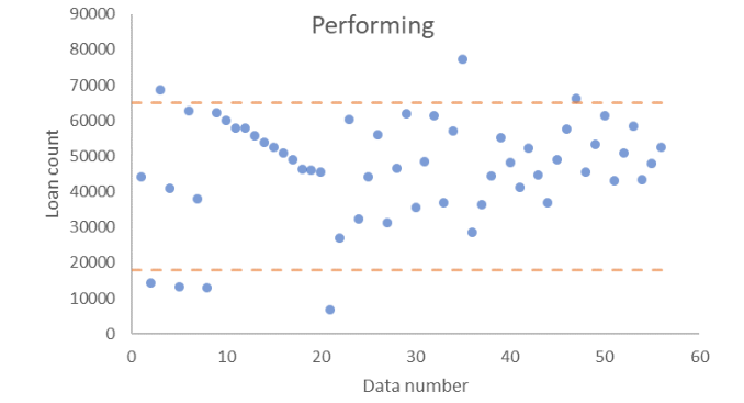
Note: The two dashed lines represent the range beyond which observations are considered to be outliers.
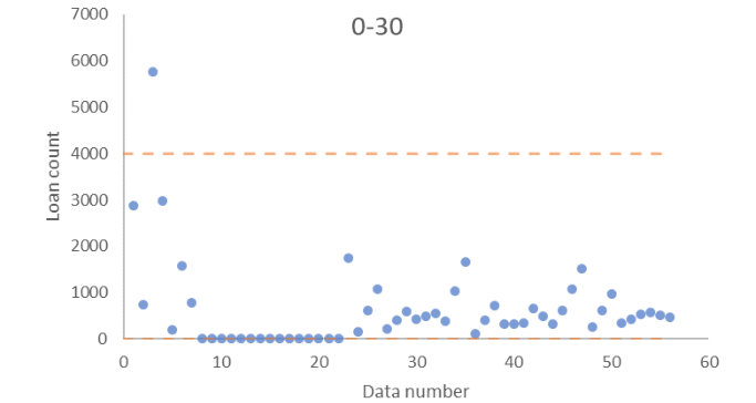
Note: The two dashed lines represent the range beyond which observations are considered to be outliers.
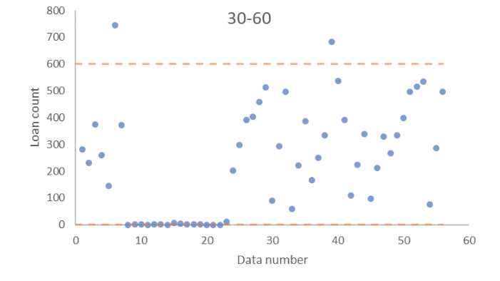
Note: The two dashed lines represent the range beyond which observations are considered to be outliers.
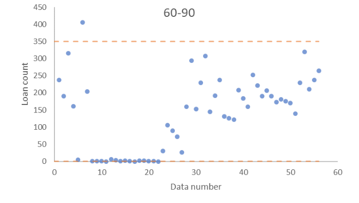
Note: The two dashed lines represent the range beyond which observations are considered to be outliers.
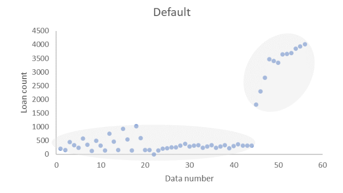
Note: Sample points form two clusters. This indicates that none of the values should be considered as an outlier.
3.2 Normalization
Normalization is an important step for many statistical learning tasks. This process scales the individual sample vector to have a norm of 1. Without scaling, the results can be distorted by the imbalanced raw values. For example, the number of loans in the Performing state are tens of thousands, while those in state 60-90 are typically just several hundred. Hence in the optimization process, changes in the state 60-90 contribute less to the objective function and it is hard to obtain sensible results. Commonly used norms include L[1], L[2]and maxnorm. In this research, we choose L[2]-norm, which is also known as the Euclidean norm. The reason is that it is often a good choice if the objective function is a quadratic form.
4. Results and discussion
Table 2 shows the PD estimates obtained using the two approaches. The first column of numbers in Table 2 contains the PDs for each bucket using the top-down approach. (Note these PD estimates are calculated using all observations from 2014 to 2018 (and not by averaging PD estimates obtained for each year.) The second column, presents the performance-based modelling results, i.e., the Markov chain approach. The third column, for comparison purpose only, contains the Markov chain results without performing data pre-processing first.
One may observe that data cleaning and scaling yields performance-based PD estimates close to those implied by the Top Down approach. The slight underestimation of the performance-based model compared to the topdown method may be resulted from two reasons:
1. We assume that the Markov chain is time-homogeneous. It is possible that the transition matrix for each year changes over time.
2. For the top-down approach, a loan can be both “performing” (0 day in arrears) and defaulted by the value in the field of Default per Basel III Definition. However, the states have to be mutually exclusive in the Markov chain method in that a loan cannot be in two states at the same time.
Although the performance-based approach seems to yield a slight underestimation, it offers the advantage that it may be implemented with readily available aggregate, performance data (of the kind commonly found in investor reports) rather than with loan level data tracked over time.
| Markov | ||||
|---|---|---|---|---|
| chain | ||||
| without | ||||
| data | ||||
| cleaning | ||||
| and | ||||
| Markov | normalizat | |||
| T | op-down | chain | ion | |
| performing | 0.91% | 0.64% | 0.67 % | |
| 0-30 days | 6.84% | 6.63% | 2.13% | |
| 30-60 days | 26.58% | 23.7 8% | 11.48% | |
| 60-90 days | 46.99% | 44.08% | 24.66% | |
| >90 days | 100.00% | 100.00% | 100.00% |
5. Conclusion and future work
In this research, we compare performance-based modelling, i.e., the Markov chain approach based on aggregate data on arrears buckets, with Top Down approaches. Our analysis and illustrative implementation on SME loan data from Caixabank suggests that the performance-based approach yields PD estimates consistent with those implied by the standard Top Down method.
Note that, in performing the comparison, we categorise loans by arrears bucket alone. It would be straightforward to implement the approach breaking the sample of loans down by sub-categories say by region in order to obtain models that more closely resemble practical Top Down models such as those employed in IRB banks. Here, we focus on the simple case in which all loans are treated as falling into one category in order to facilitate a simple comparison of the two methods.
A limitation of the performance-based approach here implemented is that the Markov chain is assumed to be time-homogeneous. In future research, it may be worth relaxing this assumption.
References
Moore, D. S. and G.P. McCabe (1999) Introduction to the Practice of Statistics, 3rd ed. New York: W. H. Freeman.
Tukey, J. W. (1977) Exploratory Data Analysis, Addison-Wesley.
Zimek, A. and P. Filzmoser (2018) “There and back again: Outlier detection between statistical reasoning and data mining algorithms,” Wiley Interdisciplinary Reviews: Data Mining and Knowledge Discovery. 8 (6): e1280.
Risk Control Limited 13-14 Dean Street London W1D 3RS +44 (0)203 307 0730 www.riskcontrollimited.com