

Abstract
This paper proposes a variant of the Arbitrage Free Approach (AFA) (developed by Duponcheele et al. (2013)) applicable when the available inputs are risk weights alone. This Simplified AFA, together with the AFA itself, offer a consistent set of approaches for regulatory capital calculations that can be used by investor or issuer banks without relying on agency ratings. The consistency of the AFA and SAFA has the significant advantage of eliminating the cliff effects that occur with the Modified Supervisory Formula Approach (MSFA) and the Simplified Supervisory Formula Approach (SSFA) recently suggested by the Basel Committee. The latter are based on different assumptions and so may imply quite different capital for a given securitisation tranche.
SECTION 1 - INTRODUCTION
The Basel Committee’s recently published proposals for securitisation regulatory capital include several approaches that place different informational demands on users. The most elaborate approach, the Modified Supervisory Formula Approach (MSFA) (set out in BCBS
(2012) and detailed in BCBS (2013a)), requires, as inputs, detailed exposure level information on the securitisation pool. The information required includes the default probability (), mean loss given default (), exposure at default and the systemic sector correlation () (dependent on its regulatory asset class) for each individual asset. In practice, it is unrealistic to expect all banks calculating securitisations capital to have individual asset. It is even more unrealistic to expect that they will all be able to estimate access to certified estimates of the Basel parameters (i.e , and ) for each these quantities, especially when they are not originators, while satisfying the rigorous data standards of the Internal Ratings Based Approach (IRBA).
In particular, investor banks (whether IRBA or Standardised Approach (SA) banks) typically have relatively little detailed information of the type required by regulators on underlying pool assets. Even when they have data on the majority of a pool’s exposures, having less complete information on a minority of assets would be sufficient to preclude use of the MSFA.
Furthermore, even for originating banks under the IRB approach, for certain regulatory asset classes, capital is specified directly in the form of a risk weight, , and in such cases there supervisory slotting criteria for the Project Finance asset class (which includes infrastructure is no possibility of accessing or or separately. For example, under the Basel 2 financing, key to the real economy), or for other Specialised Lending assets class, the banks apply directly a risk weight, .[3] For these reasons, in their proposals, the Basel authorities have supplemented the MSFA with the Simplified Supervisory Formula Approach (SSFA). Use of the SSFA requires that users know the total regulatory capital under the so-called Standardised Approach that pool exposures would attract if they were held on balance sheet (i.e., the so-called KSA[4]).
Finding its roots in BCBS (2001), the SSFA was later developed and applied in the United States for trading book securitisations. The SSFA allocates capital to different tranches of a securitisation using a simple exponential smoothing. Tranches are allocated capital equal to their par value if their detachment point is less than KSA. If the attachment point is greater than KSA, they are assigned a fraction of KSA determined by an exponential smoothing function that allocate more to mezzanine than to senior tranches.[5] The exponential weighting function employed, though reasonable, is ad hoc and has no theoretical justification.
As already mentioned, the SSFA has been applied in the United States for calculating trading book capital for securitisations. In that application, the calibration employed implies that total capital for all tranches in a securitisation equals 1.5 times the level of capital the pool assets would attract if held by the bank on balance sheet under the Standardised Approach. In the new use now envisaged by the Basel Committee (BCBS (2012)), namely for banking book securitisation capital, the ratio has been boosted to 2.5 times. (Note that for an IRB bank the ratio of pre- to post securitisation capital would be still greater because the Standardised Approach calculation for on-balance-sheet assets is, in many cases, more conservative than the corresponding IRB calculation.) The main motivation for calibrating the SSFA to imply a multiple of 2.5 times is apparently that it is then in most cases more conservative than the MSFA.
There is a widespread industry perception that the capital levels implied by the MSFA are higher than is economically justified, especially for long maturity securitisations. To arrive at its very conservative capital charges, the MSFA includes expected losses as well as unexpected losses in its definition of capital. The expected losses are not the regulatory definition of expected losses used in IRB, but instead are calculated inclusive of a conservative risk premium and cover a period up to the minimum of (i) five years or (ii) the contractual maturity of the deal. While the SSFA does not include an explicit maturity adjustment, the degree of conservatism it embodies is also extremely high.
The fact that the MSFA and the SSFA are not derived from a coherent, unified underlying theory implies that the levels of capital they imply are only roughly comparable. Small changes in the availability of data on the underlying pool that oblige a bank to use the SSFA on the entire pool instead of the MSFA may, therefore, imply a sizeable jump in capital levels, i.e., a “cliff effect”[6].
As an alternative to the MSFA, Duponcheele, Perraudin and Totouom-Tangho (2013) propose a closed form solution for calculating the capital of securitisation tranches, known as the ‘Arbitrage-Free Approach’ (AFA). In order to avoid capital arbitrage when portfolios exhibit heterogeneity and/or low granularity, Duponcheele et al. (2013) set out an approach (termed ‘Option 2’ in the paper). To implement the AFA, a bank must know the 3 Basel parameters (, , ) associated with each underlying asset in the pool.[7] ‘Option 2’ was developed in recognition of the fact that allowing banks to base capital on a securitising extreme “bar-bell” type poolsingle number, , may permit them to engage in capital arbitrage, in particular by [8]. While it is important to reduce scope for this type of capital arbitrage, it is worth noting that such aggressive structures represent a minuscule part of the securitisation market and are tackled anyway by regulators exercising their judgement when faced with such transactions[9].
Just as the MSFA is accompanied in the Basel proposals with a less informationally demanding alternative, namely the SSFA, one may ask how one might simplify the AFA to of each individual assetpermit banks to calculate capital without full information on the regulatory [10]. Answering that question is the topic of this paper. , and
Building on the simple closed form ‘Option 1’ described in Duponcheele et al (2013), in the sections below, we present a capital formula designed for handling securitisation tranches when the level of information on pool assets consists of Standardised Approach risk weights. The resulting approach is termed the ‘Simplified Arbitrage-Free Approach’ or SAFA.
As mentioned above, a simplified approach is particularly important for investor/sponsor/dealer banks. Taking as input a single number[11] that summarises underlying pool capital, a simplified approach would enable banks to calculate the capital requirements of tranches without having to rely on rating agencies. This is an obligation under Dodd-Frank and is in line with a stated objective of BCBS (2012): to reduce reliance on rating agency credit assessments.
If the AFA framework and the SAFA framework were both made available to banks, the problems around so-called mixed pools (in which IRB parameters are available for some exposures while, for others, only Standardised Approach information is available) could be addressed. In this case, using the ‘Option 2’ of Duponcheele et al (2013), one could calculate capital for the two types of exposure by working out their respective capital contributions, either with the AFA or with the SAFA, to notional structures with theoretical homogeneous sub-pools. In this way, both heterogeneity and mixed pool issues can be managed at the same time.
The rest of the paper is organised as follows. Section 2 analyses the SSFA and shows in what respects it deviates from the four principles for devising securitisation capital approaches discussed in Duponcheele et al (2013). Section 3 derives a formula for securitisation capital under our proposed SAFA and discusses a further simplification of the SAFA undertaken as to make it monotonic[12], the Monotone SAFA (MSAFA). Section 4 presents illustrative calculations using different capital formulae. Section 5 analyses the link between the well known, capital relief arbitrage may be obtained by securitising bar-bell portfolios. In this case, the ‘good’ granular credits generate the granularity necessary to flatten the SFA distribution, ensuring that the ‘bad’ credits receive relatively favourable treatment. 9 Some regulators have actually disallowed the use of the SFA on specific transactions and have required banks to use the RBA instead. 10 Note that the regulatory requirements on PDs and LGDs under the IRBA framework are much more demanding than simply estimating a PD and LGD for each position. 11 The current SFA formula takes as input the aggregate pool capital (KIRB including expected loss). The minimum IRB requirement standards require that, to calculate KIRB, banks have access to data standards enabling them to compute regulatory PDi and LGDi for each underlying asset. If this data were to be made available to investors, the SFA would be quite akin to using a single risk weight number for the allocation of capital to the tranches. 12 By ‘monotonic’, we mean that the risk weight of a more junior tranche is always greater or equal to the risk weight of a more senior tranche, regardless of its thickness.
Appendix provides details of how to implement the SAFA and MSAFA and additional parameter of the SSFA and the ∗ parameter of the SAFA. Section 6 concludes. The technical material.
SECTION 2 – IS THE SSFA A SIMPLIFICATION OF THE SFA?
Contrary to a common view, the Simplified Supervisory Formula Approach (SSFA) is not a simplified version of the existing SFA. Instead, it is a direct descendant of the original Supervisory Formula (SF), presented in the Basel Committee’s October 2001 working paper on securitisation capital (see BCBS (2001)). In that document, the following Supervisory Formula was proposed. Let and denote the attachment and detachment points of a securitisation. Let denote the reference capital level (including expected loss) on the underlying pool. For a premium factor, , and a parameter satisfying the equation 1/1 − !"#$% = , the capital requirement denoted '( of a tranche attaching above is given by: (1) '( = 1/ ∙ !"(*#$ − !"(+#$% The parameter is here called the ‘premium’ factor while the value of determines the distribution of total capital (equal to (1 + ) ) across tranches. An important question when the SF was first proposed concerned the appropriate size of the total capital of all the tranches equalled 20% more than the capital the assets would attract premium and the Basel Committee proposed a calibration of 20%. This ensured that the prior to securitisation. Pykhtin and Mingo (2002) analysed the Basel 2001 proposal by analysing the correlation between the bank’s portfolio and the securitised assets. They argued that an appropriate value of lies in the 3%-11% range[13]. was not based on a theoretical model but reflected the belief that capital should be The exponential smoothing of the additional capital (over and above ) in the SF concentrated on the mezzanine tranches rather than the senior tranches. The exponential function was a simple function that accomplished this. The fact that the exponential function converges rapidly to zero, however, implied extremely low capital for the more senior tranches, and, in a subsequent paper (see BCBS (2002)), the Basel Committee revised their earlier SF proposal by including a floor capital level.
Furthermore, the original SF was superseded in subsequent Basel proposals by the Supervisory Formula Approach. This was derived from an explicit theoretical model in which the credit quality of exposures in both the bank portfolio and the securitisation pool are assumed to be driven by the same Single Asymptotic Risk Factor. The extreme cliff effect that this assumption implies for mezzanine tranches was mitigated by the somewhat questionable device of assuming that attachment points of tranches are random.
In the latest incarnation of the SF, i.e., in the SSFA, the capital that is distributed by the formula is the Standardised Approach capital aggregate, ./ (or, when there are delinquent assets in the pool, an adjusted version of ./ known as /) rather than the which was distributed by the original SF.[14] The parameter has been simplified in that there is a new " parameter addition to total capital when one goes from pre- to post-securitisation. 0 satisfying 0 =[1][2]. Here, plays a role analogous to in that it determines the Under the SSFA, for a given tranche (with an attachment and detachment points, A and , that exceed /), capital for a given tranche equals:
(2) 789:"89;< ..4/ , 6# = = >"?# Here, 6 = −/ and = max A −/, 0#.[15] It is interesting to evaluate the SSFA against the principles that should guide the development of securitisation capital formulae according to Duponcheele et al (2013). These principles are:
1. Objective statistical basis: Capital for securitisation exposures should be based on their marginal contribution to a single, widely accepted statistical measure of the bank’s total portfolio risk.
2. Neutrality: Apart from model risk or agency effect add-ons, the capital a bank must hold against a set of assets should be unaffected by repackaging these assets into other securities as is achieved through securitisation.
3. Regulatory control: Control parameters should be available that permit regulators and supervisors to achieve their objectives and exercise judgments in the allocation of capital across different types of exposure. Such parameters should reflect the economic reality of transactions so that they could in principle be calibrated from empirical data.
4. Transparency: Capital formulae should reflect in a simple way the nature of risk and be consistent with other regulatory capital approaches to facilitate comparisons and to promote transparency.
Table 1 presents an evaluation of how the SSFA measures up to these principles. Principle How the Simplified Supervisory Formula Approach Performs
2. Neutrality The SSFA could easily be modified to enforce neutrality by requiring deduction up to / 1 − # and exponential interpolation above this value of yield results similar to the AFAthe additional capital, /. In this case, a value of [16] with conservative levels of concentration = 15% would, overall, correlation ∗. the total capital of a securitisation is 50% greater than the capital the assets Instead, a large boost in capital is proposed. A value of = 50% implies that would attract if held on balance sheet by a Standardised Approach bank. A tranches. Such an approach might be justified to allow for including market value of = 50% also implies a high dispersion of capital across senior and agency risks, say in the context of US Subprime RMBS held in the trading book. But, it appears too conservative when applied to European banking book securitisation exposures for which agency risk is likely to be much less. than before. When combined with the exponential smoothing, viewed from A value of = 150% implies that capital after securitisation is 2.5 higher the perspective of the AFA, this would imply an unreasonable degree of correlation across pool exposures. An ‘overall-cap’ (even for the portion With the calibration currently proposed, the SSFA turns fundamentally away above /) is required to avoid the capital levels becoming absurd. from the notion of neutrality in its construction, even though neutrality could easily be achieved.
3. Control parameters The SSFA has a parameter which gives the percentage of additional capital that is needed above an attachment point equal to no empirical evidence has been given by the Basel Committee to justify a /. As far as we are aware,
(2002) indicates a level below 15%.level of = 50% or = 150%. The work done by Pykhtin and Mingo
4. Transparency ‘premium’, but it is disconnected from an economic description of the risk of The SSFA is transparent. The parameter can be easily interpreted as a the underlying assets.
To conclude, the capital charge formulae presented in BCBS (2012) for the SSFA is derived from the original Supervisory Formula (SF) of the initial Basel proposal for securitisation (BSBS (2001)). The SSFA adopts a level and distribution of capital above / which is hard outcomes that arise. Another approach, as simple and transparent as the SSFA, that respects to justify empirically. When = 150%, caps are required to mitigate the unreasonable the principles listed above would be preferable.
SECTION 3 – THE SIMPLIFIED AFA (SAFA)
In this section, we set out a simplified version of the AFA developed by Duponcheele et al. (2013). The simplifications take the form of permitting inputs that demand less regulatory information about the underlying assets. The approach is sufficiently simple that it could serve as the basis of capital calculations for banks that typically have little data on pools and where such data is available, it is often not of the quality required in the IRBA rules for onbalance-sheet capital calculations. The Simplified AFA or SAFA we describe could serve as a substitute for the use of external agency ratings.
The AFA is stated in Duponcheele et al (2013) as follows, with A being the attachment point and D the detachment point of the tranche:
* Capital= ELThick(A,D,PD'α,ρ ,LGD)−ELThick(A,D,PD,'ρPool,LGD) +MRC (3)
Where, depending on the IRBA asset class: * ρPool = ρSector + 1(− ρSector) ρ
−1 −1 α = − N ( ) N (999.%)
−1 −1

1− ρ

PD'= PD×MatAdj(M ,PD)
PD'α = PDα ×MatAdj(M,PD) MRC = 6%×(PD'α⋅LGD− PD'⋅LGD) 1(− A) 1(− D) ELThick (A,D,P,ρ,LGD) = ELSeniorTranche(A,P,ρ,LGD) − ELSeniorTranche(D,P,ρ,LGD) D − A D − A LGD× N[2](X,P,ρ,LGD) − X × PDTranche(X ,P,ρ,LGD) ELSeniorTranche(X,P,ρ,LGD) = 1− X
−1 −1 N[2](X ,P,ρ,LGD) ≡ N[2](N (P), N (PDTranche(X ,P,ρ,LGD)) , ρ)
![Equation: −[1] −[1] X N (P) − 1− ρ⋅ N LGD](/api/media/file/the-simplified-arbitrage-free-approach-eq-3-300x62.png?prefix=media)
(X , P, ρ, LGD)= N

ρ
![Equation: 1+ (M − 5.2().011852−.005478 ln(P)) MatAdj(M , P) = [2] or 1 depending on the IRBAasset class](/api/media/file/the-simplified-arbitrage-free-approach-eq-5-300x34.png?prefix=media)
1−5.1(.011852 − .005478 ln(P))

(4)
The maturity adjustment MatAdj is equal to that currently used in the IRBA on-balancesheet loan rules.
The above formulae are derived for a securitisation with a homogeneous pool. Using poollevel information, Duponcheele et al (2013) set out how to apply the approach to cases with heterogeneous pools (in their ‘Option 1’) by replacing, in the above formulae, PD'α with (KIRB + EL/)' LGD where KIRB is the Basel II pool asset capital inclusive of maturity adjustment, EL' is the total pool expected loss inclusive of maturity adjustment and LGD is the total estimated mean loss for the pool assets. Similarly, PD' is replaced with EL /' LGD.
Using individual loan-level information, for heterogeneous pools, Duponcheele et al (2013) suggest (see their ‘Option 2’) calculating capital contributions for individual pool exposures based on the capital that would be implied by a notional homogeneous pool securitisation * tranche with ρ and ρi,Pool replaced with granularity-adjusted versions[17].
Since calculating the inputs for both Options 1 and 2 of Duponcheele et al (2013) requires access to detailed individual pool exposure level information, the list of inputs is: PDi Asset default probability for each exposure LGDi Asset loss given default for each exposure * ρ Concentration correlation ρSector,i Systemic sector correlation for each exposure Mi Asset maturity for each exposure EADi The exposure weight of each exposure
Suppose that, instead, either (i) the risk weights (RWs) rather than the PDs and LGDs of each asset or (ii) the average PD and LGD of the pool are available, one may ‘reverse engineer’ the relevant inputs. Specifically, one may proceed (as we shall describe below) by inferring the following parameters: PDα Stressed pool default probability PD Pool default probability LGD Pool mean loss given default * ρ Pool concentration correlation[18] ρSector Pool systemic sector correlation
One may then employ them as inputs to the equation (5) with PDα being a parameter.
* Capital= ELThick(A, D, PDα, ρ , LGD)− ELThick(A, D, PD, ρPool, LGD) + MRC (5)
To infer the above AFA input parameters from risk weights RWs, first, note that conditional on probability of pool exposures is given by: L=MN (the systemic risk factor) equalling its 99.9% confidence level, the default
(6) >?PQQRST?PQQR ?UJPQQR O = Here, 6 is the total unexpected loss for the pool of assets (better known as the Basel II IRB capital for the pool assets), V is the total regulatory expected loss for the pool of mean loss given default for the pool assets. assets (inclusive of maturity adjustment) and is the weighted average estimated
Returning to how one may proceed given risk weight alone, one may define: (7) W .X×Z.4 6W = inclusion of a scaling factor. In the IRB approach, the scaling factor is 1.06We suppose here that the risk weight makes allowance for model risk through the [19]; in this case, [\], the Model Risk Scaling Factor would also be equal to 1.06.[20] conditional probability of default employed as an input in the AFA (under Option 1) with: To implement the AFA when only risk weights are known, one may replace the
(8) >? ^ST? ^ ?UJ ^ O = up table using broad regulatory asset categories. For example, for corporates, the current If the value W is not known, it may be supplied by the regulators in the form of a look- IRB-Foundation approach defines regulatory mean LGDs as shown in Table 2.
Framework Type
Wholesale – Corporate, Sovereign, Bank Junior Claim 75% Retail –Mortgages[22] Prime 25% Retail –Mortgages Non-Prime 45% Retail – Qualifying Revolving All 85% Retail – Other Retail All 85% Others All 45% distribution of capital assigned to the senior tranches. Such a function could be written as: When the value VW is not known, it may be set by the regulators, as an add-on to boost the
(9) VW = W × 6W Here, pool level expected losses are set equal to a fixed proportion of the risk weight of the pool, where the weight W is set by regulators for the broad regulatory asset categories. BCBS (2006) gives an illustration (paragraph 377) on how to link a supervisory expected loss to a supervisory risk weight. In this case, the proportion is: W = 8%. In effect, such a value would imply that the marginal value at risk of the asset is 1.08 times the 6W. In other words, we distribute with ∗, 1.08 times the of the asset.[23] a look-up table such as those in Table 2 and an approach to inferring expected losses as in Given 6W, W, and VW as defined by knowledge of risk weights and the use of equation (8), one may infer O as the key input to the capital formula. To calculate tranche-level expected losses (i.e., the second term in the bracket in equation (5)) requires that one know the pool correlation, . As shown in equation (4), in the AFA model, the intra-pool correlation is = W + 1 −W#∗, where W is analogous to , the systemic correlation in the IRB approach. To derive it, it requires identifying the systemic correlation W appropriately. For some asset classes, such as residential mortgages or qualifying retail exposures, this determination is straightforward as the correlation takes a fixed value for all individual exposures. The choice is more difficult when, under the Basel assumptions, the individual exposure correlation depends on the probability of default of the assets. This default probability is assumed to be unavailable to a bank implementing the SAFA. To be broadly compatible with BCBS (2006), we suggest that a lookup table be employed including values such as those set out in Table 3.
For exposures under the wholesale framework, the granularity adjustment would be consolidated exposures. In this case: calculated as in paragraph 633 of BCBS (2006), with hi being the effective number of + where 7∑m,m⊂k T/Jm< (10) + m,m⊂k jk 7∑ T/Jm < W = hi = For securitisation pools comprising retail assets only, granularity is very high, and there is no need to include a granularity adjustment, therefore, W = 0%. For the wholesale framework, if the effective number of consolidated exposures can be shown[30] to be greater than 100, then W = 0%, otherwise W = 1/hi. Table 4 summarizes the granularity adjustments we propose.
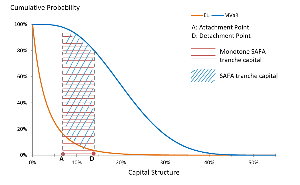
A graphical representation of the Simplified AFA is shown in Figure 1. The area between the Marginal VaR and the Expected Loss curves equals the Unexpected Loss. This area equals the Pool Risk Weights times 8%. The model may then be thought of as distributing this area over thin tranches according to their attachment point (i.e., their seniority).
Figure 2 exhibits the capital and Expected Losses for a discretely thick tranche and shows how the Monotone SAFA is constructed by adding to the Unexpected Loss the regulatory Expected Loss.
Finally, if required, one may further modify the SAFA to impose the monotonicity of capital charges. If the regulatory expected loss (PD x LGD), including any related maturity adjustment, is included in the total amount of capital, both the AFA and the SAFA become monotonic. We refer to those versions as the Monotone AFA (MAFA) and Monotone SAFA (MSAFA).
Figures 1 and 2 illustrate the concepts just discussed. Figure 1 shows the total capital on all tranches (before any adjustment for monotonicity), equal to the pool risk weight multiplied by 8%, displayed as the area between the Marginal VaR and the Expected Loss curves. In effect, given the Risk Weight, the SAFA model attributes an amount of capital to the different tranches depending on the choice of the ∗ parameter. Figure 2 shows the SAFA-implied capital for a discretely thick tranche (with attachment and detachment points as shown in the figure) as the area between the MVaR and EL curves between A and D. The Monotone SAFA capital for the same tranche simply adds to the SAFA capital the area under the EL curve between A and D.
systemic correlation, as the systemic correlation impacts only the distribution of the expected A key advantage of the Monotone SAFA is that there is no need to have a proxy W for the losses and not the distribution of the marginal value at risk.
Moreover, with a monotone version, there is no need to change the existing operational regulatory processes that currently exclude securitisation tranches when assessing whether margins on the bank’s assets are sufficient to cover the regulatory expected loss of the bank.
SECTION 4 – ILLUSTRATIVE CALCULATIONS OF THE SAFA
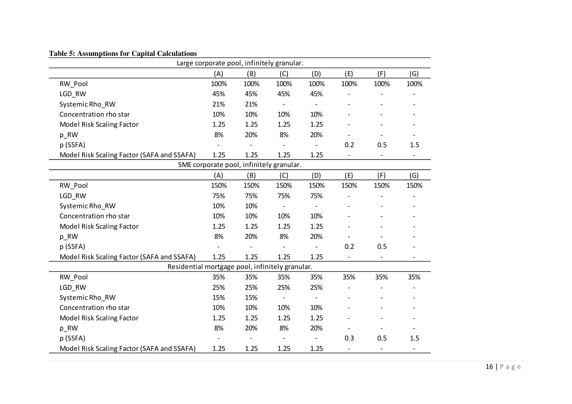
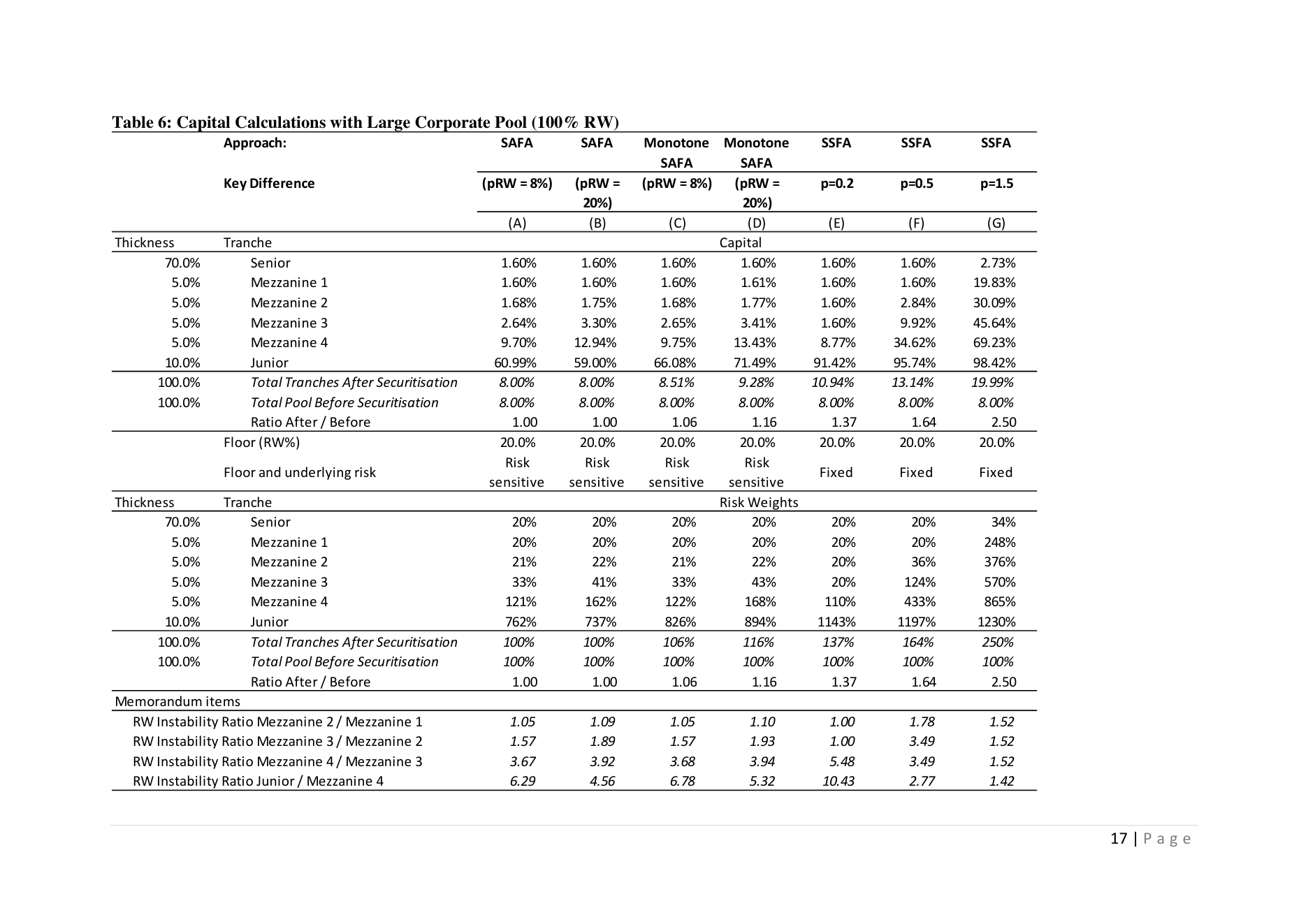
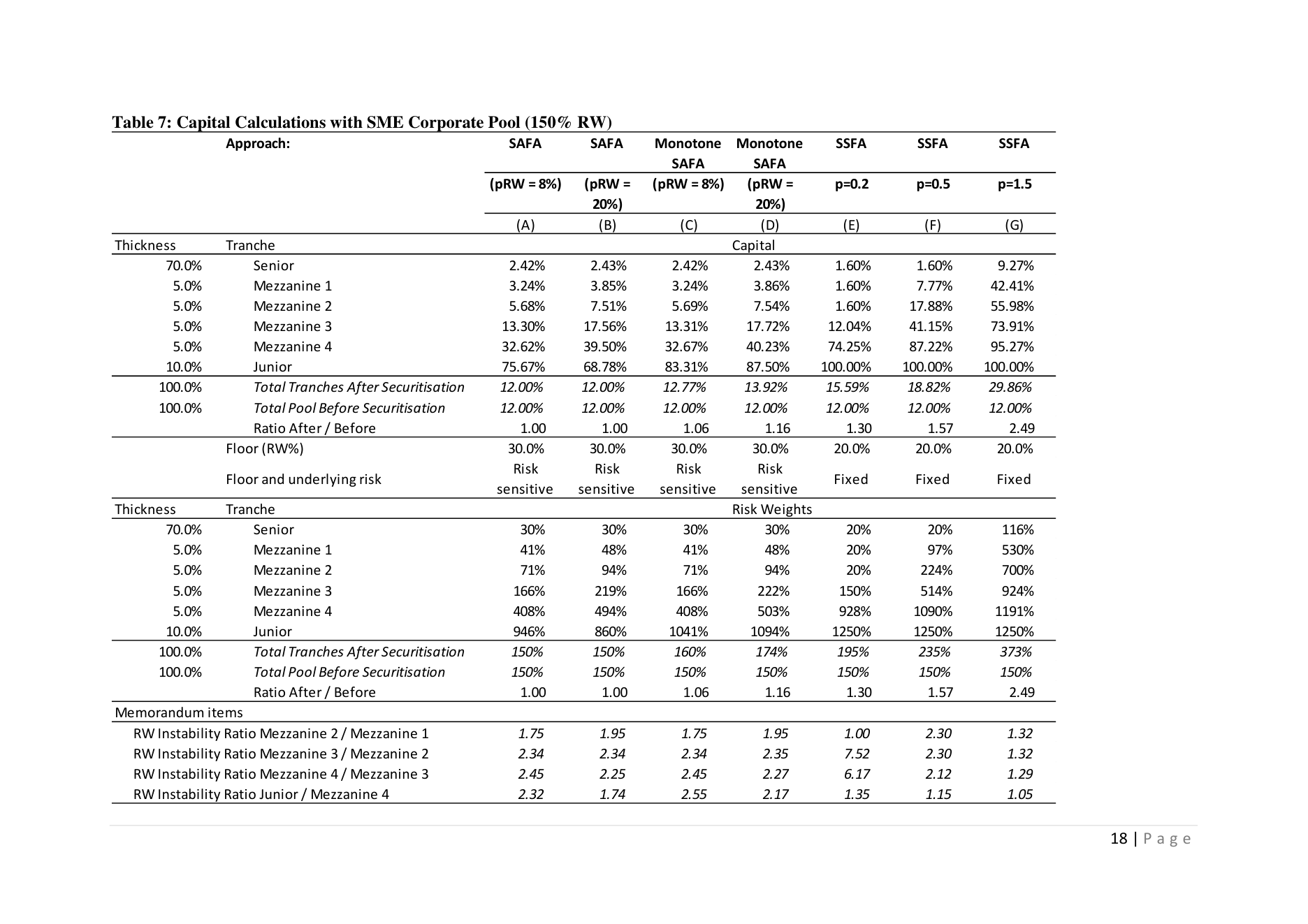
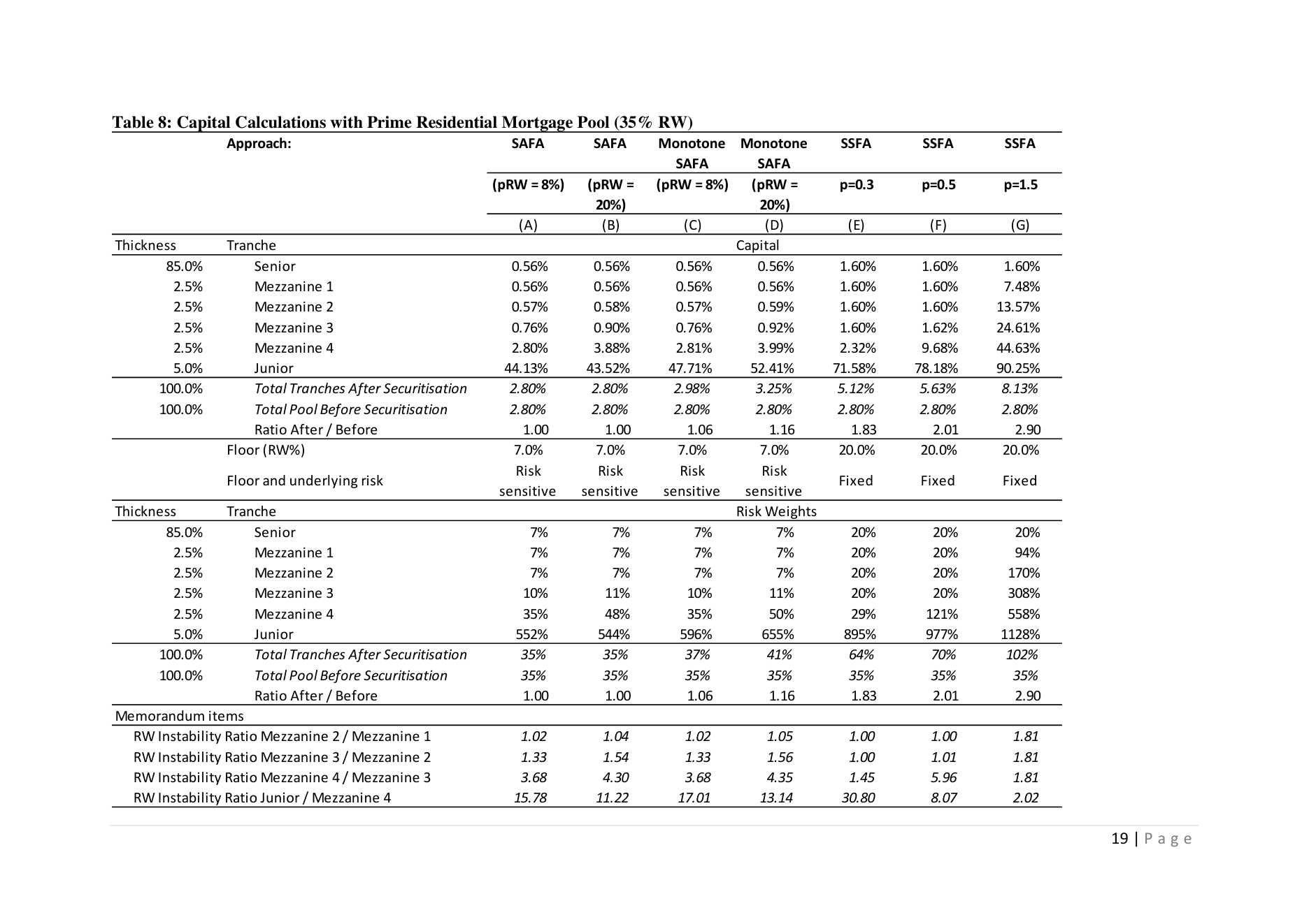
This section presents illustrative calculations using different capital formulae, for 3 broad categories of assets using standardised risk weights. The three cases examined are a) large corporates with RWs of 100%, b) SMEs with RWs of 150% and c) residential mortgages with RWs of 35%. The detailed assumptions employed in the calculations are set out in Table 5. All numbers are produced using a concentration correlation ∗ of 10%, as this section is not concerned with the sensitivity to this parameter, but rather with (i) the sensitivity to W, (ii) the impact of monotonicity, and (iii) the sensitivity to the premium parameter of the SSFA. Table 6 presents results for a securitisation with a pool of large corporate assets. We employ a standardised proxy for W of 45% in this case. Table 7 shows results for a pool of SME 75%. Table 8 presents results for a pool of RMBS assets for which we used a standardised corporate assets in which case we employ a conservative standardised proxy for W of proxy for W of 25%. For each category, we analyse how capital is affected by the inclusion of regulatory expected loss. We use values for W of 8% and 20%. In the case of the SAFA, the proxy parameter effect of reducing slightly the capital of junior tranches, distributing capital towards the junior W creates regulatory expected losses below the Unexpected Loss distribution, and has the mezzanines. Capital for the senior mezzanines is relatively insensitive to this parameter. raises the capital for the junior mezzanines (Mezzanine 4 and Mezzanine 3) by 33% and 25% To illustrate this, in the case of the large corporate pool, increasing W from 8% to 20% respectively, whereas the capital levels for the senior mezzanines (Mezzanine 2 and Mezzanine 1) increase by 3.9% and 0.1% only. For residential mortgage pools, the capital increases for the junior mezzanines (Mezzanine 4 and Mezzanine 3) are 39% and 19%, respectively, whereas for the increase for senior mezzanines (Mezzanine 2 and Mezzanine 1) have barely noticeable increases of 2.0% and 0.1%, respectively. One may note that, for the SME pool securitisation, the increase is distributed more evenly as there is a combined effect of a higher risk weight and a higher loss-given-default.
In the Monotone SAFA, the increase in capital mainly affects the junior tranche, however. The inclusion of the regulatory expected loss in the Monotone SAFA eliminates the phenomenon of decreasing capital when expected losses rise, that occurs under certain conditions. (Note that this phenomenon is already a feature of the current IRB formulae and, although counter-intuitive[33], it is managed in practice by requiring sufficient spread and/or provisions.)
In the case of the SME example, the increase in regulatory expected loss that occurs when of 946% to 860%, while increasing the capital allocated to mezzanine tranches. The W increases from 8% to 20% reduces the capital allocated to the junior tranche from a RW Monotone SAFA instead increases the RW of the junior tranche from 1041% to 1094%, by converting this increased regulatory expected loss into capital requirement. The Monotone SAFA rules out situations in which the RW of a more junior tranche will be less than that of a more senior tranche regardless of thickness.
Note that by using a Model Risk Scaling Factor of 1.25 in the SAFA formula for Standardised Approach banks, the model risk charge creates a risk-sensitive floor of 20% of the underlying risk weight. This compares with a non-risk sensitive floor from the SSFA of 20% under the current Basel proposals. If 20% is the level of model risk that regulators regard as sensible for an average corporate portfolio risk weighted at 100%, it can be shown that 20% is too high for residential mortgages (it should be 7%), while it can be argued that it is too low for SMEs (it should be 30%). The problem arises because the floor in the SSFA is not risk sensitive.
SECTION 5 – RELATION BETWEEN SSFA AND SIMPLIFIED AFA
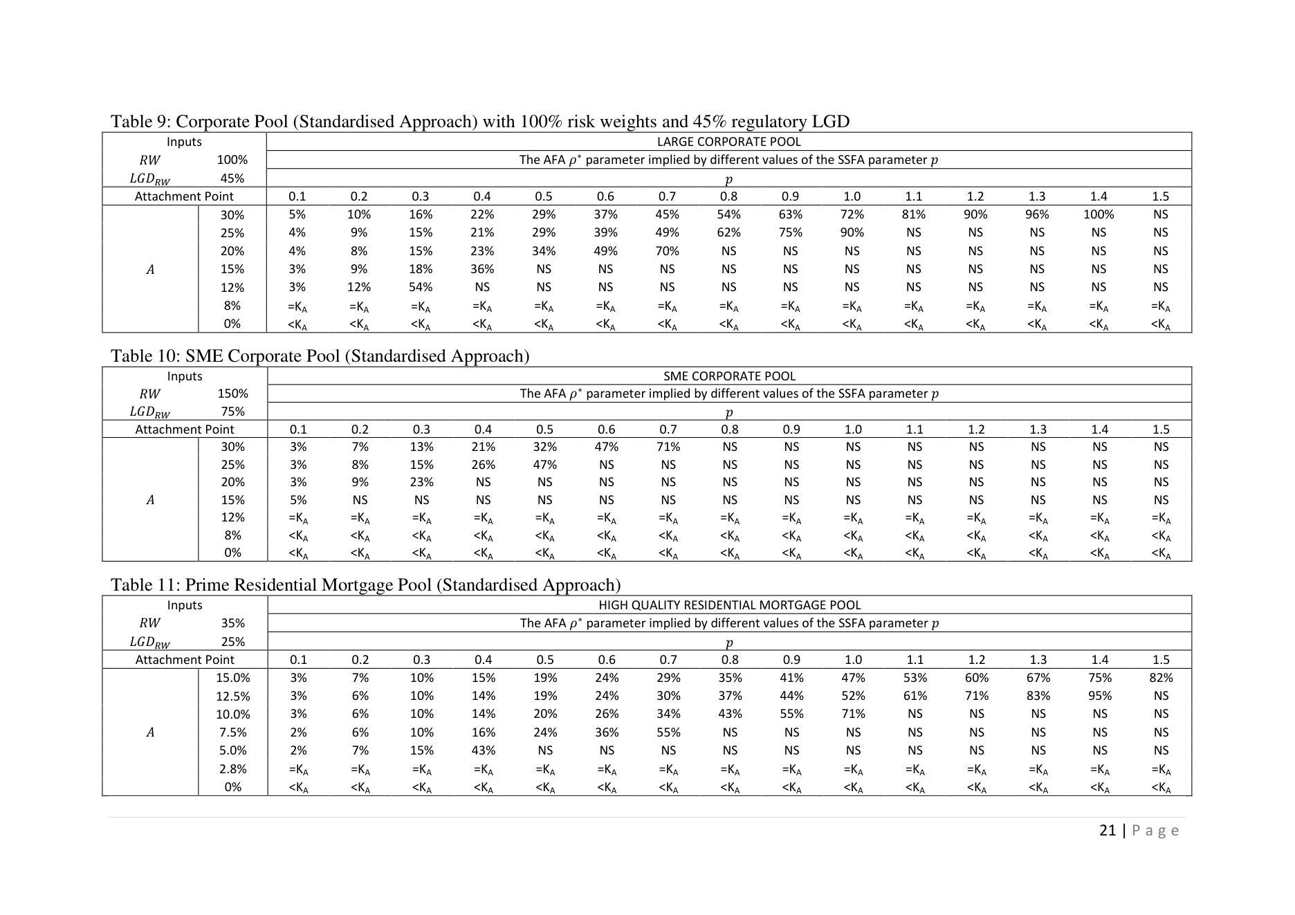
In this section, we provide a reconciliation of the SSFA and AFA parameters, showing how reasonable values for the AFA parameters (about which one may adduce empirical experience) provide intuition for appropriate values for the SSFA calibration.
The capital for a thin tranche in the SSFA for an attachment point L is given by:
(11) ..4/ , S# ≈ =∗? " Here, 0 =[1][2]. For the same attachment point, the AFA yields the following capital value:
(12) js*t Ju2v"js*t;xyw vz{∗ /4/ , S# ≈N r z"{∗ | equation below: For a given , one may derive the ∗ that yields the same capital value by solving the implicit
(13) /4/ , S# = ..4/ , # After some manipulation, the solution reduces to solving a quadratic equation and hence the development in given in the Appendix 4, but can be presented numerically below. implied ∗ value is available in closed form if a solution exists. The full mathematical
Tables 9 to 11 below show the results of such calculations for pool containing (i) investment grade large corporate loans, (ii) SME corporate loans and (iii) prime mortgage pools. For investment grade corporate pools, it can be seen in Table 9 that a ∗ of about 10%, corresponds approximately to a SSFA parameter value of = 0.2. The SSFA market risk rule in the US is currently employs the value = 0.5, and this would correspond to an implied ∗ of 25% for high attachment points. Note, however, that there is hardly any ∗ parameter that could justify an SSFA parameter value of = 1.5, as currently proposed in Basel (2012). The set of equations is not two factor model like the Pykhtin-Dev/AFA model. numerically solvable, or in other words setting = 1.5 cannot be approximated in a standard As one may observe from Table 10, for SME corporate pools, ∗ parameter of about 10% corresponds to a SSFA parameter value of = 0.2. The SSFA market risk rule in the US, currently using = 0.5, would correspond to an implied ∗ of 35% for high attachment numerically solvable, i.e., the SSFA is incompatible with a two-factor model. points. Setting = 1.5 as in the proposed Basel (2012), the set of equations is not For RMBS (see Table 11), the level of ∗ of about 3%, which corresponds to this asset the magnitudes proposed by Pykthin and Mingo when the original SSFA was developed. class[34], corresponds to an SSFA parameter value of = 0.1. Such a value is of the order of
A ∗ value of about 10% corresponds to a value of = 0.3. The SSFA market risk rule in the US, currently using = 0.5, would correspond to an implied ∗ of 21% for high attachment incompatible with a two factor model and is not numerically solvable. points. But setting = 1.5 as in the proposed Basel (2012), the set of equations is
SECTION 6 – CONCLUSION
In a recent speech[35], Wayne Byres set out the principles that should guide the design of regulatory policies, stating that such policies should be:
1. Comprehensive, yet simple;
2. Strong, but not burdensome;
3. Risk-based, yet easy to understand and compare;
4. Flexible and adaptable, yet consistently applied;
5. Suitable for normal times, but founded on the lessons from crises;
6. Built on consensus, but also on the broadest possible engagement; and
7. Utilising appropriately the relative strengths of both regulation (rules) and supervision (oversight).
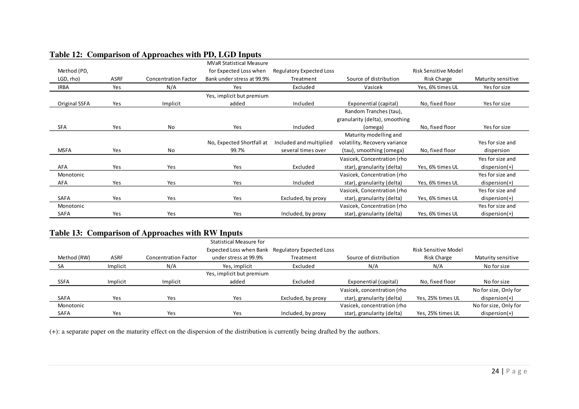
In our view, the current proposals for securitisation capital contained in BCBS (2012) do not adhere to these broad principles. The SSFA has some desirable characteristics, specifically transparency and simplicity for investors, originators and dealers, but fails in other regards. The MSFA is deficient in most of the dimensions identified by Byres.
Following feedback from the industry, there has been extensive discussion of several aspects of the proposed securitisation capital framework (for example on calibration, simplicity of use, risk-sensitivity) but so far there has been somewhat less focus on Byres’ point 4, i.e., on consistency. In particular, the lack of consistency between the MSFA and the SSFA is a significant weakness of the current proposals since it implies sharp discontinuities in capital levels depending on what information is available to a bank.
In this paper, we have developed a simplified version of the Arbitrage Free Approach proposed in Duponcheele et al (2013). Because the so-called Simplified AFA is coherent in underlying assumptions with the AFA itself, the two approaches combined offer a consistent set of approaches that may be used by investor or issuer banks.
Both the AFA and the SAFA, with or without monotonicity, are easily adaptable to real-life securitisation situations, with or without granularity, with or without heterogeneity, with or without mixed pools, with SA and/or IRB data. In its simplest form, the Monotone SAFA asset pool. could be constructed with just one user-supplied input: the risk weight of the underlying
The resulting AFA and SAFA approaches are comprehensive yet simple, conservative but not burdensome, risk-based yet easy to understand and compare, flexible yet consistently applied, suitable for normal times but built on lessons from the crisis, built on consensus with a broad engagement but leaving the regulators in control.
![Pool Risk Weights[32]](/api/media/file/the-simplified-arbitrage-free-approach-fig-1.png?prefix=media)
| Framework | Type | ebc | ||||||||
|---|---|---|---|---|---|---|---|---|---|---|
| Wholesale | Corporate, | Sovereign, | Bank | 24 | 21% | |||||
| Wholesale | SME25 | 10% | ||||||||
| Wholesale | Other26 | 12% | ||||||||
| Mortgages27 Retail – | Prime/Non-Prime | 15% | ||||||||
| Retail – Qualifying | Revolving28 | All | 4% | |||||||
| Retail – Other | Retail29 | All | 10% | |||||||
| Others | All | 12% | ||||||||
| 23 However the | value of | is | sensitive | to the | underlying | parameters. | Below | are | examples of | |
| W | ||||||||||
| regulatory asset | classes, designed | to | enable | a | comparison | between | the IRB and | Standardised | approaches: | |
| V | 6 | f | g# | \G# | ||||||
| W | W | |||||||||
| Large Corporates | 1.25% | 45% | 0.6% | 21% | 7.9% | 98% | 100% | |||
| Residential Mortgages | 1.00% | 25% | 0.3% | 15% | 2.8% | 33% | 35% | |||
| SME Corporates | 3.30% | 75% | 2.5% | 10% | 13.6% | 148% | 150% | |||
| It can be seen that | a value | of | = 8% | is adequate | for large | corporates | and | residential | mortgages | |
| W | ||||||||||
| probably insufficient | for SMEs, | where | = | 20% is a more | appropriate | order | of | magnitude. | ||
| W | ||||||||||
| 24 | ||||||||||
| See Basel (2006), | paragraph | 272. | Normally, | the values | for individual | exposures | lie | between | 12% (for low | |
| credit quality assets) | and 24% | (for high | credit | quality assets). | A broad | ‘BBB-‘ | portfolio | would | = give: | |
| W | ||||||||||
| 25 | ||||||||||
| See Basel (2006), | paragraph | 273. | The values | required by | the Basel | rules are | between | 0% and | 4% below | |
| corresponding | corporate | correlation. | Hence, | a reasonable | value would | be 2% | below | 12% (the | value for low | |
| credit quality | corporates), ie.: | = | 10%. | |||||||
| W | ||||||||||
| 26 | ||||||||||
| The category “Other” | would | include | specialised | lending | for example. | |||||
| 27 | ||||||||||
| See Basel (2006), | paragraph | 328. | ||||||||
| 28 | ||||||||||
| See Basel (2006), | paragraph | 329. | ||||||||
| 29 | ||||||||||
| See Basel (2006), | paragraph | 330. | Normally, | the Basel | rules require | values | between | 3% (low | credit quality | |
| assets) and 16% (high | credit | quality | assets). | A | reasonable | “middle-ground” | value | would be: | = 10%. | |
| W |

References
Basel Committee on Bank Supervision (2001) “Working Paper on the Treatment of Asset Securitisation,” Bank for International Settlements, October.
Basel Committee on Bank Supervision (2002) “Second Working Paper on Securitisation,” Bank for International Settlements, December.
Basel Committee on Bank Supervision (2006) “International Convergence of Capital Measurement and Capital Standards: A Revised Framework, Comprehensive Version,” Bank for International Settlements, June.
Basel Committee on Bank Supervision (2012) “Revisions to the Basel Securitisation Framework,” Consultative Document, Bank for International Settlements, December.
Basel Committee on Bank Supervision (2013a) “Foundations of the Proposed Modified Supervisory Formula Approach,” Working Paper 22, Bank for International Settlements, January.
Basel Committee on Bank Supervision (2013b) “The Proposed Revised Ratings-Based Approach,” Working Paper 23, Bank for International Settlements, January.
Duponcheele, Georges, William Perraudin and Daniel Totouom-Tangho (2013), “A Principles-Based Approach to Regulatory Capital for Securitisations,” BNP Paribas / RCL memo, 21st April 2013, available from the authors.
Pykhtin, Michael and John Mingo (2002) “Apportioning Economic Capital Among Tranches of an Asset Securitization – the Basel 2001 Proposals,” Revised, April 3.
Appendix
A1: STEP-BY-STEP IMPLEMENTATION OF MONOTONE SAFA
This ‘monotone’-simplified version does not require a proxy for the systemic correlation to determine the expected loss contribution, but uses a regulatory multiplier for the expected loss to ensure that the unexpected losses are appropriately distributed.
With the following inputs:
• the risk weight of the pool, (including of any scaling factor) class (see tables);
• the regulatory estimate of loss-given default W set by regulators for the asset
• the new ‘stressed’ correlation ∗, set by regulators for the asset class;
• the multiplier to include regulatory expected loss, [T? = 1 + W
• the model risk scaling factor [\] (1.25 for SA and 1.06 for IRBA)
• for the tranche , given its effective attachment point G, and effective detachment point Calculate:
(A1.1) WPQQR .X×Z.4 6 = (A1.2) = W [36] (A1.3) >?PQQR×Z; \′ = ?UJPQQR (A1.4) = ∗ (A1.5) \( G# = 0 ( G, \ , , # (A1.6) \( # = 0 ( , \ , , # \( G, # = 0 ( G, , \( G#, \( #, \′ , , # (A1.7) (A1.8)[37] %'W = \( G# ∙\( G, # + [\] −1# ∙ 6# (A1.9) $'W = $ −$G# ∙ %' ( Final coherence check (prior to adjustments): ∑ $' should be equal to 12.5 × . The VBA function 0 ( and 0 ( are given at the end of this paper. ∑m7?UJ ^,m∙T/Jm< 36[37] This part can be changed with a weighted average pool Because of the non-deduction of EL and the addition of the MRC, for the most junior and ultra thin tranches, such that =
A2: MONOTONE SAFA WITH GRANULARITY ADJUSTMENT
This variant takes the granularity effect and its impact on the distribution of unexpected loss contribution. This is particularly relevant for those non-retail securitisations (typically nongranular CMBS)
For exposures under the wholesale framework, the granularity adjustment would be consolidated exposures. In this case: calculated as in paragraph 633 of BCBS (2006), with hi being the effective number of + (A2.1) m,m⊂k 7∑ T/Jm< + 7∑m,m⊂kT/Jm < W = jk ℎ hi = In that case the implementation is like in Appendix 1-A but replacing the stressed correlation by: (A2.2) = ∗ + W 1 −∗# Please note that for securitisations of retail or SME underlyings, granularity is very high, and there is no point in attempting a granularity adjustment in the Vasicek distribution. For retail exposures: W = 0%.
A3: STEP-BY-STEP IMPLEMENTATION OF THE SAFA
This simplified version takes into account the expected loss contribution and the granularity effect and its impact on the distribution of unexpected loss contribution. In contrast to the Monotonic Simplified AFA, it then removes the expected loss contribution from the capital of the securitisation tranches.
With the following general inputs:
• the systemic correlation W, set by regulators for the asset class (see tables)
• W a regulatory estimate of expected loss as a proportion of unexpected loss ( 0 #
• the new ‘stressed’ correlation ∗, set by regulators for the asset class
• the model risk scaling factor [\] (e.g. 1.25 for SA and 1.06 for IRBA) With the following parameters for each asset :
1. the risk weight (including of any scaling factor)[38]
2. the exposure at default VG (see tables);
3. the regulatory estimate of loss-given default W, set by regulators for the asset
Calculate for the asset, the asset dependent value:
• the implied unexpected loss of the asset:
(A3.1) Wm .X×Z.4 6W, = 38 In IRBA, this would be = 12.5 × × 1.06
Calculate pool parameters:
• the weighted average implied unexpected loss of the pool:
(A3.2) ∑ 7>? ^,m∙T/Jm< ∑ T/Jm 6 =
• the implied expected loss of the pool:
(A3.3) V = W ∙ 6
• the implied loss given default of the pool:
(A3.4) m ∑ 7?UJ ^,m∙T/Jm< ∑mT/Jm =
• the implied probability of default of the pool:
(A3.5) T?PQQR ?UJPQQR ′ =
• the implied stressed probability of default of the pool:
(A3.6) >?PQQRST?PQQR ?UJPQQR \′ =
• the effective number of consolidated exposures in the pool, if relevant: + (A3.7) 7∑m,m⊂kT/Jm< + m,m⊂k 7∑ T/Jm < hi =
• the granularity adjustment: (A3.8) jk W = Coherence check: the unexpected loss contribution to Bank of the pool should be equal to:
(A3.9) %W, = \′ ∙ − ∙ = 6 Calculate for each tranche, the tranche-dependent and pool-dependent values: For the tranche with the effective attachment point of the tranche G, and the effective following intermediary steps: detachment point of the tranche , the contribution of the to the tranche need the
For the Expected Loss Component:
• the pool correlation , is given by: (A3.10) = W + 1 −W# ∙∗
• the Vasicek granularity adjusted pool correlation:
(A3.11) ′ = + W ∙ 1 − #
• the probability of default of the tranche boundaries ( G# and ( #: (A3.12) ( G# = 0 ( G, ′ , , ′ # (A3.13) ( # = 0 ( , ′ , , ′ #
• the loss given default of the tranche ( G, #: ( G, # = 0 ( G, , ( G#, ( #, ′ , , ′ # (A3.14)
• the Marginal Contribution of the tranche to the Expected Loss of the Bank: (A3.15) %['(V=MN = ( ∙ ( For the Stressed Expected Loss Component:
• the Vasicek granularity adjusted stressed correlation:
(A3.16) ′ = ∗ + W ∙ 1 −∗#
• the stressed PD of the tranche boundaries \( G# and \( #: (A3.17) \( G# = 0 ( G, \′ , , ′ # \( # = 0 ( , \′ , , ′ # (A3.18)
• the Stressed LGD of the tranche \( G, #: \( G, # = 0 ( G, , \( G#, \( #, \′ , , ′ # (A3.19)
financial stability confidence level (FSCL=99.9%):
• the Marginal Contribution of the tranche to the Value at Risk of the Bank, at the
(A3.20) %['(0=MN,4.? = \( G# ∙\( G, # For the Model Risk Charge Component:
• the Marginal Contribution of the tranche to the Model Risk Charge of the Bank: (A3.21) %['(['=MN = 7 [\] −1# ∙%W, < Apply the Basel II formula for the 3 Unexpected Loss Components:
(A3.22) %'W = %['(0=MN,4.? −%['(V=MN + %['(['=MN
Multiply by the thickness to move from percentage notation (applied to the tranche’s notional) to ‘dollar’ notation (applied to the pool’s notional):
(A3.23) $'W = $( −$G(# ∙ %' (A3.24) $W, = $1 ∙%W, ( should be equal to $W, . Final coherence check (prior to adjustments): ∑ $' The VBA function 0 ( and 0 ( are given at the end of this paper.
A4: BASIC VBA FUNCTIONS The function given below: 0 ( G, , , # and 0 ( G, , ( G#, ( #, , , # are 0 ( G, , , # =
(A4.1) js* 1#"z"{∙js*tR2 v G ≥, ℎ ( G# = 0% 0 < G < , ℎ ( G# = h r z{ | G = 0, ℎ ( G# = 100% 0 ( G, , ( G#, ( #, , , # G ≥, ℎ ( = 0% ( # = ( G# ∙ −G 0 ≤G < , ℎ ( = + | −G −G# ∙ rg , ( G#, # −g , ( G# ( #, # where g , ( #, # ≥, ℎ g , ( #, # = 0% (A4.2) = 0 < < , ℎ g , ( #, # = h7h" #, h"7 ( #<, z< = 0, ℎ g , ( #, # = with h , , # being the bivariate cumulative standard normal distribution function[39].
39 The h # function is easily implementable in Excel using VBA.
A5: THE LINK BETWEEN P OF THE SSFA AND ¡∗ OF THE AFA The SSFA Capital Charge ..4/ for a given tranche is determined by the following formula:
(A5.1) 789 :"89 ;< Here: ..4/ , 6# = = >"?# = G −/ 6 = −/ 0 = −1 /
(A5.2) £ / = 1 −# ¢ + For most assets, it is 8%. W is the percentage of the underlying portfolio that is currently K¥ is the weighted average Basel risk-based capital requirement of the underlying portfolio. defaulted or in serious delinquency. A is the tranche attachment point, D is the detachment point. p is 0.5 for securitisations and 1.5 for re-securitisations.
Capital under the SSFA for a very thin Tranche is given by the following equation.
(A5.3) ..4/ , # ≈ =∗? Under the AFA, capital for a similar thin tranche is as follows.
(A5.4) js*t Ju2v"js*t;xyw vz{∗ /4/ , S# ≈N r z"{∗ |
The implied AFA correlation for thin tranches may be derived as follows.
(A5.5) js*t Ju2v"js*t;xyw vz{∗ /4/ , S# = ..4/ , # ≈N r z"{∗ | = =∗?
(A5.6) ¦ h"7[2]< −h" t?UJv z∗ = h" =∗?#z1 −∗ (A5.7) α∗ + z∗ + ¨ = 0 where α = h" © L + h" =∗?# « β = −2h" © L « h"7[2]< γ = h"7[2]< − h" =∗?# This equation has a real solution if and only if the discriminant is positive, i.e., if:
(A5.8) ¦ ∆= −4°¨ = 4h" =∗?# ©h" t?UJv + h" =∗?# − h"7[2]<« "±S√∆ (A5.9) , > √∆ O z∗ = "±"√∆ , − > √∆ O
Notes
[1] Dr. Georges Duponcheele is Head of Banking Solutions Private Side, BNP Paribas. Dr. William Perraudin is a Director of RCL and Adjunct Professor of Imperial College, London. Dr. Daniel Totouom-Tangho is in Credit Quantitative Research, BNP Paribas and is Adjunct Associate Professor of Financial Engineering at New-York University (NYU-Poly). Correspondence should be addressed to the authors at georges.duponcheele@bnpparibas.com, william.perraudin@riskcontrollimited.com or daniel.totouom- tangho@bnpparibas.com.
[2] The authors thank from BNP Paribas: Fabrice Susini, Antoine Chausson, Duc Dam Hieu, Alexandre Linden, Iuliana Dincov and Eric Silie, and from other institutions: Alexander Batchvarov, Shalom Benaim, Kamel Benhaddou, Vivien Brunel, Norbert Jobst, Dherminder Kainth, Stephan Meili and Alastair Pickett for their contribution, their numerous and helpful comments. Duponcheele and Totouom-Tangho thank Manish Chandra and Kaiwen Xu for ensuring that time was made available to develop this solution. All errors are ours. The views expressed are the authors’ own and not necessarily those of BNP Paribas nor those with whom we had discussions or their firms.
[3] In this case, even if IRB banks were to have access to default probabilities and loss given default means, no supervisory systemic asset value correlation ρi is available. An infrastructure asset in a securitisation pool precludes use of a formula that requires the 3 Basel parameters (PDi,LGDi,ρi) for each underlying pool asset.
[4] An adjustment is made for delinquent assets.
[5] If KSA lies between the attachment and detachment points, a weighted average of these two approaches is employed.
[6] The term ‘cliff-effect’ is used in the context of jumps in capital requirements. Within securitisation, there are
[3] broad categories of jumps. Firstly, in the AFA paper, we refer to the term ‘cliff-effect’ in the context of a mathematical discontinuity caused by the use the ASRF model, designed for diversified banks, to determine the capital requirement of concentrated securitised portfolios. Secondly, in this paper, we use the term ‘cliff- effect’ to indicate that a change in the applicable formula due to a small change in available regulatory information, for the same underlying capital, creates large jumps in the capital requirement of the entire securitised portfolios. Thirdly, in the context of the RBA, the term ‘cliff-effect’ refers to the fact that senior tranches are capital deducted when their rating drops to below BB-, requiring in the process several multiples of the capital requirement of the underlying portfolios.
[7] A step-by-step implementation of ‘Option 2’ is provided in Appendix 6 of Duponcheele et al (2013).
[8] By assuming random attachment points, the SFA formula attempts to rectify the cliff effect in capital that follows from the assumption of a single asymptotic risk factor driving both bank portfolio and securitization pool. The random attachment point device reduces but does not eliminate the cliff effect, however, and, as is
[13] Their conclusion is consistent with analysis of the link between the p parameter of the SSFA and the ρ* of the AFA in Section 6 below. 1. Objective The SSFA does not change the statistical criterion for risk for the underlying statistical assets since it employs the underlying capital as an input. It is risk sensitive (if basis we leave aside the deduction below regarded as a distributive function. / and the floor). The SSFA may be 14defined to be delinquent if it is “90 days or more past due, subject to a bankruptcy or insolvency proceeding, in Specifically, if a fraction of the pool, W is delinquent, then, / = 1 −#./ + 0.5 . A pool asset is the process of foreclosure, held as real estate owned, had contractually deferred interest payments for 90 days or more, or were in default.” (See BCBS (2012), page 22.)
[15] When, < / , the tranche Risk Weight is 1250%. When G > /, the Risk Weight is 12.5 times ..4/. 2"/ J" 2# J"/# . When < / < G, the Risk Weight is set equal to: 12.5 J"/ + 12.5..4/
[16] Although results of such SSFA with p=0.15 would probably be correct for the most senior tranches and most junior tranches, they would remain inadequate for mezzanine tranches. * *
[17] These are respectively: ρ + δi 1(− ρ ) and ρi,Pool + δi 1(− ρi,Pool) . In the current context, i.e., in an Option 2 calculation, the δi should be calculated on a consolidated obligor basis as: EADi / EADPool . Note that, in contrast, in an Option 1 calculation, it is appropriate to calculate the adjustment based on the approach used in BCBS (2006), paragraph 633, i.e., based on: ∑ EADi[2] / ∑( EADi ) .
[18] Again, granularity adjustments may be added to the correlations as described in footnote 14 and in the Appendix of Duponcheele et al (2013).
[19] In the IRB Approach, the capital requirement is the UL, increased by 6%, via the scaling factor.
[20] In the Standardised Approach the floor for AAA securities is a 20% RW (calibrated with an underlying corporate portfolio with 100% RW); this would be equivalent to setting the Model Risk Scaling Factor equal to 1.25. This reflects the calculation 100% x (1-1.25)/1.25 = 20%. In other words, by setting an MRSF of 1.25, this could give a model risk charge (equivalent to a risk sensitive floor) of 20% RW for large corporate underlyings (100% RW), 30% RW for SME underlyings (150% RW) and 7% for residential mortgages underlyings (35% RW).
[21] As in IRB Foundation Approach (see paragraphs 287 and 288, Basel (2006)).
[22] This is based on examples provided in Basel (2006), Annex 5.
[33] In IRB, when there is a large amount of regulatory EL in an asset, the UL cannot go higher than 1-EL.
[34] See page 18, Duponcheele et al (2013)
[35] “Simplicity, Risk sensitivity and Comparability: the Regulatory Balancing Act,” Wayne Byres, 25-26 February 2013. . ∑mT/Jm equation A1.8 can go over 1250%. This numerical issue disappears with the thickness of real tranches. A numerical control could be added to ensure that no tranches go over 1250% risk weight.