

Abstract
This paper examines how the capital required for securitisation tranche exposures varies as the maturity of the securitisation increases. We investigate for different maturities the appropriate capital for (i) loan pools, (ii) securitisation deals as a whole (i.e., all the tranches within a given deal), and (iii) individual tranches of differing seniority.
This issue is highly topical because the Basel Committee’s recent proposals on regulatory capital for securitisations include an expected loss component that is highly sensitive to maturity. An alternative proposal, the Arbitrage Free Approach (AFA), advanced by the industry (see Duponcheele et al (2013)) builds maturity effects into the capital formulae in a very different way.
The paper makes the following points:
1. We develop a new multi-period version of the AFA and use show that it is equivalent to the 1-period AFA of Duponcheele et al (2013a) when maturity-adjusted parameters are included.
2. The AFA is capital neutral in the sense that securitisation capital for all the tranches of a deal equals the IRBA capital inclusive of maturity adjustment. We show that IRBA maturity adjustment is quite conservative when compared to the capital implied by an industry-standard ratings-based Monte Carlo credit portfolio model.
3. Using the same Ratings-based Monte Carlo model, we show that with suitable maturity adjustments, the AFA yields an appropriate dispersion of capital across tranches of different seniorities while maintaining capital neutrality.
SECTION 1 – INTRODUCTION
Duponcheele et al (2013a) derive a simple, closed form model of securitisation capital. That model includes maturity adjustments at the level of the total deal capital (in line with the maturity adjustments in the on-balance sheet Internal Ratings Based Approach (IRBA) rules of Basel II). Duponcheele et al (2013a) left open, however, the issue of whether input parameters that influence the dispersion of capital across tranches of differing seniority should be adjusted for maturity.
This paper derives a simple, multi-period model of securitisation capital fully consistent with the original AFA which provides a rigorous justification for maturity adjustment in the AFA’s inputs. As with the original AFA, the model may be aligned perfectly with the IRBA capital at different maturities and hence remains ‘Arbitrage Free’.
The AFA parameter maturity adjustments implied by the analytical model include adjustments to both correlation and default probability inputs. In both cases, the adjustments are based on extremely simple, closed-form expressions.
The resulting model may be compared with the Modified Supervisory Formula Approach (MSFA) recently proposed by the Basel Committee (see BCBS (2012)). This model also allows explicitly for credit risk in securitisations in a multi-period setting. However, it cannot be solved in closed form and is therefore implemented using a sequence of approximations including fitting the moments of a beta-distribution.
Importantly, the total deal capital implied by the MSFA bears no direct relation to KIRB, the capital required in Basel II if pool assets are held on balance sheet. Hence, if implemented, the MSFA would introduce dramatic inconsistencies between the regulatory capital required for the same risks packed in different forms.
Both the model of this paper and the MSFA are simple models with limited detail in the modelling of multi-period risks. It is helpful and instructive to compare the capital from such models with realistically complex models. In the second half of the paper, we therefore calculate capital for a set of deals using a multi-period Ratings-based Monte Carlo model generalised to permit the risk and capital analysis of exposures to securitisation tranches. We show that, suitably adjusted, the multi-period AFA implies very similar capital charges.
The Monte Carlo model we employ is based on the industry-standard ratings-based credit portfolio model methodology popularised by J.P. Morgan (1997). Note that ratings based credit portfolio models of this type are widely used for calculations of trading book Incremental Risk Charges under the post-crisis Basel 2.5 regulations set out in BCBS (2009).
We extend the ratings-based methodology to permit analysis of portfolios including securitisation tranches using the Longstaff-Schwartz regression approach. This was employed in Longstaff and Schwartz (2001) for pricing American options and was first applied to credit portfolio risk assessment by Peretyatkin and Perraudin (2004).
The approach is designed to cope with situations in which the a Monte Carlo is being employed to estimate a payoff in the future but that future payoff itself depends on a future price that, itself, may only be estimated through a Monte Carlo. To avoid the nested Monte Carlo problem that arises (and which is computationally infeasible), the approach involves estimating a conditional (regression-based) pricing function via a preliminary Monte Carlo and then using it in a subsequent Monte Carlo, in our case to generate VaRs and Marginal VaRs.
The analysis of this paper is topical because the Basel Committee’s recently published proposals for securitisation capital are based on capital formulae (in particular the MSFA) that are, controversially, highly sensitive to maturity. Some of the conservatism comes from the use of layers of conservative approximation within a model that cannot be solved in close form. In addition, the basis of capital employed in the MSFA differs from the ‘Unexpected Loss’ notion employed in the Basel II on-balance-sheet capital rules in that an additional, highly conservative expected loss is included.
The Committee’s objective in including expected loss in this way is not entirely clear. One motivation may have been that adding a conservative measure of expected loss mitigates a major weakness of the Supervisory Formula Approach (SFA) which was the forerunner of the MSFA under Basel II.
The SFA implies capital for mezzanine tranches that is excessively sensitive to changes in pool credit quality. This sensitivity (commonly termed the “cliff effect”) means that quite minor losses on the pool could generate substantial increases in capital. The sensitivity also reportedly encouraged capital arbitrage by banks[3].
The solution offered by the MSFA is to add a further conservative layer of capital for securitisation tranches over and above their Unexpected Loss by including a conservative measure of Expected Loss. These Expected Losses are over-conservative (a) because they cover not only potential losses for up to five years but also (b) because they are computed inclusive of a risk premium of the kind used in pricing credit risk sensitive instruments. Particularly for long-maturity securitisations, the effect is to mitigate the cliff effect significantly.
However, since expected losses (inclusive of a risk premium) grow at a rate more than in proportion to maturity, this solution to the cliff effect conundrum immediately implies very substantial increases in capital for longer dated tranches.
A second possible justification for including Expected Losses as a form of capital is that the cash-flow waterfall of some securitisations allow for the deferral of coupon payments on some mezzanine tranches as the pool deteriorates well before the tranche actually defaults. If coupons are deferred in this way, there will be insufficient interest margin on the tranche in question to cover the tranche-level expected losses.
Such coupon-deferral features are only found in some deals and, in any case, while they disadvantage mezzanine tranches, they actually reinforce the credit quality of senior tranches. We believe the appropriate treatment of this issue in the capital rules is to include a test (i) of whether coupon deferral is possible and if so (ii) whether adequate interest margin exists at the tranche level. We intend to return to this issue in a future study.
The remainder of this paper is organised as follows. Section 2 reviews the 1-period AFA developed in Duponcheele et al (2013a). Section 3 introduces a simple multi-period extension of it. Section 4 looks at how capital on loan pools increases with maturity. Section 5 examines maturity adjustments as they affect the total deal capital for a securitisation. Section 6 looks at the impact of maturity on the appropriate dispersion of capital across tranches of differing maturity. Section 7 reconciles results obtained using the multi-period AFA with those implied by the Ratings-based Monte Carlo model. Section 8 concludes. Appendices provide the data used in the calculations, a description of the Ratings-based Monte Carlo model employed in the paper and a systematic description of the equations of the simple, multi-period version of the AFA.
SECTION 2 – SECURITISATION CAPITAL IN THE 1-PERIOD AFA
As in Duponcheele et al (2013a), suppose that a perfectly granular securitisation pool contains 1-year loans. Default on each loan is triggered when an associated standard Gaussian latent variable falls below a threshold denoted: . The latent variable for the ith loan, , satisfies:
(1) √ √ √ √ √
Since is standard Gaussian, the probability of default for the ith exposure is:
( ) (2)
In equation (1), is a factor common to all the exposures in the pool but orthogonal to the common factor driving the bank portfolio, namely: . The random variables and are assumed to be standard Gaussian and and are fixed parameters in the unit interval.
Substituting, one may define the following expressions:
(3) √ √ (4) √ (√ √ √ ) (5) ( )
The parameter then equals the pairwise correlation of latent variables for individual exposures in the pool.
Consider losses on a tranched position. If pool losses are denoted , losses on a tranched position equal (i) zero if , (ii) , if , and (iii) if .
If is only marginally larger than , when , the tranche will default and the recovery rate will be zero. Hence, expected losses on such a tranche just equal the tranche’s default probability which in turn equals the probability that losses on the pool exceed the attachment point A. As Duponcheele et al (2013a) note, this implies the expected loss, ( ) for a thin tranche attaching at is:
( ) √ ( ) ) (6) ( ) ( √
To obtain the expected losses (denoted ELThick(A, D) ) of a discretely thick tranche with attachment point A and detachment point D, one must integrate the above expressions for the marginally thin tranche from A to D. This yields:
1( − A) × ELSenior(A) − 1( − D) × ELSenior(D) ELThick (A, D) = (7) D − A LGD× N[2] − X × PDTranche(X ) ELSenior(X ) = 1− X
−1 −1 (8) N[2] ≡ N[2] (N (PD), N (PDTranche(X )) , ρPool )
![Equation: −[1] −[1] X N (PD) − 1−ρPool ⋅ N](/api/media/file/eq-132-300x44.png?prefix=media)
LGD

PDTranche(X ) = N

ρPool

In the above equation, ELSenior(X ) equals the expected loss for a senior tranche with attachment point X and ( ) is the bivariate cumulative standard normal distribution function.
To calculate the marginal VaR (at an α-confidence level) of a thin tranche held within a wider bank portfolio, following the insight of Gourieroux, Laurent and Scaillet (2000), one may calculate expected losses conditional on the common factor driving the bank portfolio, −1 N ()α . equalling its α- quantile,
−1 N ()α , the stressed default probability of pool exposures is: Conditional on equalling
−1 −1

PDα= N (9)

1− ρ

and the conditional pairwise correlation between pool assets is:
* ρPool,α = ρ (10)
Replacing and where they appear in equations (7) and (8) with and , respectively, yields expressions for the thin and thick tranche marginal VaRs.
Unexpected Loss-based Capital, denoted K(A, D), for a thick tranche attaching at A and detaching at D , may be expressed as:
* K(A, D) = ELThickTranche(A, D | ρ, PDα) − ELThickTranche(A, D | ρPool, PD) (11)
In Duponcheele et al (2013a) it was proposed that the above expression (which was derived from a 1-period model) be used to calculate tranche capital for tranches of differing maturity by setting the stressed default probability equal to:
(12) ( ) rather than the expression in equation (9). Here, is the Basel II IRBA capital for the pool assets (exclusive of expected loss but inclusive of maturity adjustment) and is the total pool IRBA expected loss inclusive of maturity adjustment. LGD is the mean loss given default for the pool assets.
Use of an adjusted stressed default probability in this way ensured that the approach is ‘arbitrage free’ in the sense that, for any maturity, the total capital for the deal equals the IRBA on-balance-sheet capital for the pool assets, . Duponcheele et al (2013a) suggested that there might be need to adjust other inputs to the securitisation capital formula to ensure that the dispersion of capital across tranches of different seniorities was appropriate. It is to this issue that we turn in the next few sections.
SECTION 3 – SECURITISATION CAPITAL IN THE M-PERIOD AFA
Some General Results
We begin by considering securitisation capital within a general theoretical setting. Consider capital calculated at date 0 for a VaR horizon equal to 1 year. Let cumulative loan losses from 0 up to a terminal date of M years on a securitisation pool be denoted: LM .
The value at date t =1 of a tranched exposure to the securitisation pool, with attachment point A and detachment point D , is denoted V[1]. We suppose that the tranched exposure forms part of the portfolio of a bank and that the credit quality of the bank’s portfolio at date 1 depends on a random variableYB1, . We indicate the α-quantile of the distribution of YB1, as
−1 Qα≡ N ()α .
We suppose for simplicity that interest rates and coupon rates are zero. We use Et [] to denote the expectations operator at time t with respect to actual distributions. As is standard, we assume that securities prices may be expressed as expectation with respect to risk adjusted * E or ‘risk neutral’ probabilities, and we denote the ‘risk neutral’ expectations operator as t [].
Subject to these assumptions the Unexpected Loss on the tranched position in the securitisation pool may be expressed as:
KM = E[0][]V[1] − E[0][V[1] YB1, = Qα]
* * (13) = E[0][E[1][D − A − min(D, max(L, A))]− E[0][E[1][D − A − min(D, max(L, A))] YB1, = Qα]
D * D * = ∫A Gα,M (LM )dLM − ∫A GM (LM )dLM
Note that the expectations of loan losses that appear in the second line of (13) are calculated with actual distributions in the first period (0 to 1) and inclusive of risk premiums in subsequent periods, 2, 3,..., M. Correspondingly, Gα*,M (LM ) and GM* (LM ) are distribution functions for cumulative losses up to date M inclusive of risk premiums in all periods except the first.
The first equality in equation (13) says that the UL-based capital equals the difference between (i) E[0][]V[1] , i.e the expectation E[0][] at time t = 0 of future price of the position V[1] E V Y Q E at t =1 and (ii) [0][[1] B1, = α], the expectation [0][] at time t = 0 of future price of the position V[1] at time t =1, conditional on the bank’s risk factor being at it’s α-quantile level at the one year horizon, i.e., YB1, = Qα. The second equality in (13) ‘unpacks’ the expected future price and the stressed expected future price.
Line 3 in (13) follows from D − A −min(D,max(L, A) = D − min(D, L)−(A − min(A, L) and the fact that, for any random variable, L , with a distribution function, F , and density f , one
D D has E[D − min(D, L)]= 1(− F(D)) D − L f (L)dL = F(L)dL where the last equality ∫[0] ∫[0] follows from integration by parts.
The above argument is rather general in the sense that loan losses could be generated by different models. It will hold for a ratings-based model of loan losses with ratings transitions (as is widely employed for actual credit portfolio modelling by many banks) or by a multiperiod Merton style model of the type used to derive the MSFA.
Deriving Maturity Adjustments within the AFA
The two integrals in the last line of equation (13) are the counter-parts of the two expressions that make up the Unexpected Loss formula for discretely thick tranches in the AFA. The first term is a Marginal VaR and the second an Expected Loss. The difference between the two then constitutes an Unexpected Loss.
From the arguments in the last section, we can derive an explicitly multi-period version of the AFA by calculating the difference between two expectations of hold-to-maturity tranche credit losses[4]. The two expectations should use appropriate distributions. Both should employ probabilities for the evolution of risk factors in periods after period 1 and the first of the two expectations should condition appropriately on the bank stress, i.e.,YB1, = Qα.
One could accomplish this using different credit risk models but the most straightforward is to employ a multi-period Merton-type model as follows.
Suppose, the credit quality of individual loans is driven by latent variables describing the underlying values of the borrowers’ assets, . We suppose that:
(14) √ √ √ √ √
Here, , , are the levels of standard Brownian motions (with , , all equal to zero) and, hence, have discrete time increments that are normally distributed and serially independent. Since the latent variables are here taken to have normally distributed discrete time increments, it is more reasonable to suppose that they equal the natural logarithm of the borrowers’ asset values rather than the levels of these values.
Here, is the single common factor driving the credit quality of the bank’s wider portfolio while is another common factor orthogonal to . is a factor idiosyncratic to the ith borrower.
The pairwise correlation of the discrete time increments and for obligors i and j is:
(15) ( )
This equals the correlation of latent variables in equation (5). Conditional on , it is simple to show that the correlation of and is equal to:
( ) ( ) ( ) (16) ( ) ( ) ( | ) ( )
One may verify that, for , this reduces to: . For large , on the other hand, this correlation approaches the unstressed correlation, .
Adopting the above assumptions about the basic factor structure of the model, we assume that the ith loan defaults at date M if and only if where ( √ ) so that is the M-period default probability under the natural measure.
Note that in formulating the model in this way, we effectively are employing a pure Merton model (as in Merton (1974)) in which defaults are registered only at the maturity date, rather than a Black-Cox-style model (see Black and Cox (1976)) in which defaults may occur at intermediate points before full maturity. Using a pure Merton model is analytically convenient in this context. In the discussion of the Ratings-based Monte Carlo analysis below, we shall examine the issue of how outcomes are affected by allowing for intermediate defaults.
If the are the natural logarithms of the individual borrowers’ asset values, including a risk premium in the dynamics of these risk factors after the first period is straightforward. The risk adjusted process followed by the latent variable for the ith obligor becomes:
(17) ̃
Here, γ is a per-period risk premium.[5] Suppose that the historically observed default probability appropriate for -maturity assets is denoted pdM . Under the above assumptions, the ith obligor defaults between dates 0 and if a Gaussian random variable falls below a threshold as follows: ( ) . Hence, the default probability inclusive of appropriate risk premiums is:
![Equation: −[1] (M −)1 γ PDM = N N (pdM )+ (18)](/api/media/file/eq-139-300x25.png?prefix=media)
M

The key point to grasp is that adopting the above assumptions, on a hold-to-maturity basis, defaults on the securitisation pool and on the wider bank portfolio occur when realisations of Gaussian random variables fall below cut-off points: ̃ ( ) . The correlations of these Gaussian random variables are given by: and conditional on the . Hence, the model is formally identical to the one period AFA model bank stress event by of Duponcheele et al (2013a) except with inputs PDM and rather than PD (as defined in equation (2)) and .
As in equation (9), one may derive the default probability (denoted PDα,M ) of a single obligor
−1 conditional on the bank stress event, YB1, = N ()α . This yields:

M

PDα,M = N (19)

M

However, as in the 1-period AFA, the stressed default probability, PDα,M , may be set in such a way as to ensure neutrality between on- and off-balance sheet capital, i.e., to ensure that total deal capital equals the IRBA capital charge for the pool assets. This may be achieved by setting:
KIRB PDα,M = + PDM (20) LGD
Here, KIRB is the IRBA pool capital charge inclusive of IRBA maturity adjustments.
To understand where this comes from, note that the IRBA capital formula for a single loan may be stated succinctly as: KIRB = (PDα⋅ LGD − PD⋅ LGD)MatM . Here, MatM is a parametric function of maturity, M , PD is the 1-year default probability of the loan and PDα is the 1-year default probability conditional on the assumption that the single common factor driving the bank’s total portfolio of credit exposures equals its α-quantile. The AFA as * described in Duponcheele et al (2013a) uses as inputs ρ , PD =' PD MatM and PDα'= PDα MatM .
As discussed above, one might consider employing a stressed, M-year-maturity, default probability. But unless this stressed default probability is chosen exactly as in equation (20), the total capital for assets held on-balance sheet will differ from the total requirement for all the tranches in the securitisation.
In summary, we propose that applications of the AFA employ an M-period default probability inclusive of risk premiums for years after the first year (as specified in equation (18)) and then from this infer a stressed M-period default probability using equation (20). This combination of default probability and stressed default probability is consistent with the analysis of equation (13) but also yields capital neutral results.
SECTION 4 – MATURITY AND LOAN CAPITAL
In this and subsequent sections, we present numerical calculations of capital for securitisations of different maturities. We begin by reviewing the conservatism of the maturity adjustments in the IRBA. This is a relevant issue because the AFA capital for the entire deal is aligned with the IRBA pool asset capital, i.e., KIRB . The IRBA KIRB includes a maturity adjustment which is therefore inherited in the AFA.
We first examine, in brief summary form, the findings of Kiesel, Perraudin, Taylor (2003), a paper written as part of the calibration effort on the IRBA risk charges. This paper analyses the sensitivity of capital to different aspects of the portfolio, including maturity, by calculating capital for portfolios of loans based on a standard ratings-based credit portfolio model of the type employed in this paper. The correlation structure employed is that of a single common factor. Individual loans have a common pairwise asset correlations denoted: ρ which is set equal to 20% in all cases. Results are presented for homogeneous portfolios consisting of 500 loans all having the same rating and maturity.
Note that, under these assumptions on correlations and with a homogeneous pool of assets, VaRs and Marginal VaRs (as a fraction of expected value) are equal so long as the portfolio is large enough for idiosyncratic risk to be diversified away (which is the case of a portfolio of 500 loans). Hence, the results we present may be regarded either as VaRs or as MVaRs.
Also, note that the VaRs are calculated using a portfolio loss distribution in which losses are measured as deviations from the expected future value of the portfolio. Hence, though we shall here call them VaRs (as is done in Kiesel, Perraudin, Taylor (2003)), they are equivalent to Unexpected Losses.
Two approaches to modelling recoveries are employed: (i) the Jarrow-Turnbull approach (see Jarrow and Turnbull (1995)) in which recoveries are a fraction of the default free equivalent loan (also employed in Jarrow, Lando and Turnbull (1997)), (ii) the Duffie-Singleton approach (see Duffie and Singleton (1999)) in which recoveries equal a random fraction of the value just prior to default.[6] A third approach sometimes preferred by practitioners is to suppose the recovery in the event of default is a fraction of the par value of the bond or loan. When interest rates are low, this third approach is similar to the Jarrow-Turnbull approach.
The results in Table 1 exhibit significant positive sensitivity of VaRs for high credit quality portfolios but strikingly little for low credit quality, in which case the sensitivity with respect to maturity may even be negative.
What is the intuitive explanation for these results? When credit quality is high, transition risk predominates and capital grows with maturity in the expected way. However, when credit quality is low, the jump in value that occurs upon default plays a larger role. Whether capital increases with maturity or not then depends on how one chooses to model recoveries.
Under the Duffie-Singleton approach, when default occurs, the loan value jumps down even if the credit quality just before default is low. Under the Jarrow-Turnbull approach, the loan price just prior to default is already low if the rating is low and the maturity is high. So the price jump that occurs at default is not so great. This then generates smaller capital.
Though the Duffie-Singleton and Jarrow-Turnbull approaches are probably those most commonly used in academic studies, one might argue that the practitioner approach mentioned above of employing the par value of the bond is preferable.[7] Note that using recoveries equal to the loan par will reduce (or push negative) the sensitivity of capital to maturity even more as (for a given recovery fraction) it has the effect of reducing the size of the jump from the value immediately before default to that observed after default.
The Jarrow-Turnbull approach with positive interest rates is likely to give maturitysensitivities of capital intermediate between those implied by the other two approaches. In the calculations we perform below, we use the Jarrow-Turnbull approach but perform calculations with zero interest rates, in which case it becomes equivalent to the ‘practitioner approach’.
SECTION 5 –MATURITY AND TOTAL SECURITISATION CAPITAL
On- and Off-Balance Sheet Capital
In this section, we present new results on capital for pools of loans. In some cases, we look at capital for a portfolio of loans held directly by a bank within a wider portfolio of bank loans. In others, we calculate capital for a collection of all the tranches in a securitisation again held within a wider bank portfolio of loans. One may refer to these two situations as total capital on and off-balance sheet.
We evaluate capital using a ratings-based Monte Carlo model and then compare the results (i) with the regulatory capital figures suggested by the IRBA for an asset pool and (ii) with the capital implied by the MSFA for the collection of all the tranches. Note that because the AFA is capital neutral, IRBA capital is equivalent to the capital implied by the AFA.
We conduct these calculations for portfolios of loans with maturities of 1, 2, 3, 4, and 5 years[8] and for two credit quality cases, namely a portfolio comprising BB-rated loans and a portfolio made up of BBB-rated loans. The assumptions we make about the stylised securitisations are as follows.
The VaR horizon is a year and the maturity of all the loans in the bank’s wider portfolio is three years. The maturity of loans in the structured product pool varies from 1 to 5 years and is the same as that of the structured product. There is a single common factor in the structured product pool and another single common factor in the wider bank portfolio.
1. The structured product exposure is negligibly small compared with the wider bank portfolio.
2. In the Ratings-based Monte Carlo analysis, the wider bank portfolio is assumed to consist of 500 BBB-rated loans. The securitisation pool is supposed to comprise either 200 BB-rated loans or 200 BBB-rated loans.
3. The par value of the exposures in the structured product pool is assumed to equal 7% of the par value of the loans making up the wider bank portfolio. The total par of tranches is split into 27 tranches as described by Table 2.
4. The interest rate is set to zero for different maturities. This implies that the Jarrow- Turnbull approach that we employ in recovery modelling is equivalent to the ‘practitioner approach’ of supposing the recovery is a fraction of par value.
5. The recovery rate is modelled as deterministic (to provide comparability with the assumptions in IRBA (and AFA)) and is set at 55%, a value appropriate for large corporate loans.
6. The spreads and ratings transition matrix employed in the calculations are shown in a data appendix. The spreads are estimated from a large dataset of US corporate bonds. Averages of spreads (by maturity and rating) observed weekly in the second quarter of 2007 is employed in order to provide a pre-crisis set of values. In a corresponding fashion, the rating transition matrix employed is taken from Standard & Poor’s default study including data up to 2007.
Capital Calculation Results
The results of the calculations for total capital on- and off-balance-sheet appear in Table 3. The on-balance sheet results are in the columns under “Capital for the Pool, and the offbalance sheet results are in the columns under “Capital for all Tranches”.
Column (A1), labelled “MC Capital for Pool”, shows the capital for the pool assets implied by a Monte Carlo calculation.
Column (B1), labelled “IRBA Capital”, shows the capital for the pool assets as defined under IRBA. This IRBA measure excludes the Expected Loss. As maturity increases, there is a noticeable increase of capital due to the IRBA maturity adjustment. The ratios between the entries in the column at different maturities and the 1-year capital number are simply equal to the proportional IRBA maturity adjustment. Note that the ratios of the capital numbers for maturities 1 and 5 are not equal for BBB and BB pools because the maturity adjustment in the IRBA formula depends on default probability of the exposure in question.
By construction, the implied AFA capital for the pool yields exactly the same total capital as the IRBA Capital, thus inheriting the IRBA’s maturity adjustment.
For a 1-year maturity, the Monte Carlo estimates in column (A1) are close to the IRBA capital in column (B1) (6.48% vs. 6.13% for BB and 3.04% vs. 2.75% for BBB) since the pool exposures are driven by the latent variables with the same factor structure as that assumed in the analytical AFA model. Differences here reflect sampling errors. The Monte Carlos are performed with 5 million replications but even so there is likely to be some inaccuracy as Monte Carlo estimates of VaRs calculated with a confidence level of 99.9% converge relatively slowly.
Column (C1) shows the input of the current SFA formula, which is basically the IRBA Capital inclusive of Expected Loss.
Column (D1) shows the capital implied by the MSFA model for the pool assets where the calculations are performed exclusive of the regulatory capital caps and floors.
Column (A2), labelled “MC Capital for all Tranches”, shows the sum for all the tranches in the securitisation of the UL-based capital implied by the Ratings-based Monte Carlo model. Comparing the MC capital for all tranches with the MC capital for pool, one may observe that the estimates are reasonably close being, for example, 2.76% and 3.04%, respectively, for 1-year-maturity and 4.57% and 4.39%, respectively, for 5-year-maturity securitisations with BBB-rated underlying exposures. This shows that apart from sampling error, the total capital implied by the two very different Monte Carlo estimations are consistent. This observation provides some confirmation that the Longstaff-Schwartz conditional pricing function approach that is used in the Monte Carlos for the tranche exposures are performing accurately.
Column (B2) shows total AFA capital for all the tranches in the securitisation; the numbers in column (B2) are identical to the numbers in column (B1), by construction.
The last column (D2) of Table 3 shows the total capital implied by the MSFA for the securitisation as a whole. The calculated results show a much more aggressive sensitivity to maturity than the AFA/IRBA numbers imply.
One possible justification of the aggressive maturity adjustment in the MSFA is the notion that some mezzanine tranches may suffer deferral of coupon prior to credit events affecting the tranche in order to protect the credit quality of more senior tranches in the securitisation.
In our view, this phenomenon should be addressed within the regulatory framework through including a specific test on whether sufficient excess interest is available for a tranche and whether the cash-flow waterfall rules of the deal permit coupon deferral or not. The current approach involves penalising, with no justification that is apparent to us, both mezzanine tranches for which coupon deferral is not permitted in the waterfall rules and senior tranches, the credit quality of which is actually enhanced by mezzanine or junior tranche coupon deferral!
Moreover, a comparison between the numbers in columns (D1) and (D2) shows the disproportionate effect of the fixed floor in the MSFA as currently calibrated when compared to the overall amount of capital for the pool (9.68% vs. 6.63% for BB and 5.36% vs. 2.86% for BBB for 1-year maturity).
The key result that emerges from an examination of Table 3 is that the IRBA maturity adjustments are relatively conservative. While the 1-year-maturity total capital results are similar (as, theoretically, they should be) across the three cases of AFA/IRBA, MC Capital for Pool and MC Capital for all Tranches. For the 5-year-maturity exposures, the AFA/IRBA results are higher for the BBB-rated pool exposure case and very much higher indeed when BB-rated pool exposures are assumed.
SECTION 6 – MATURITY AND TRANCHE CAPITAL DISPERSION
In this section, we examine how capital should be dispersed or allocated across tranches of different seniorities in a securitisation. The AFA has the important advantage that the sum of the capital it implies for all the tranches in a securitisation equals the capital that a bank must hold if it invests in the pool assets directly. The AFA is capital neutral in this sense whatever the maturity of the securitisation.
Being aligned with the IRBA for total capital does not necessarily imply, however, that the dispersion or allocation of capital across tranches of differing seniority implied by the use of * a fixed value of ρ in the AFA is appropriate. Furthermore, one might enquire whether adjustments should be made to the default probability used as input to the AFA.
We address these questions in this section (i) by calculating using the Longstaff-Schwartz ratings-based Monte Carlo model the appropriate UL-based capital for different tranches in our stylised securitisation deal and then (ii) by comparing the implied dispersion with that implied by the AFA with its inputs adjusted in different ways.
Before looking at long-lived deals, we verify (see Figure 1) that the Ratings-based Monte Carlo model yields accurate estimates of the capital of different tranches for a 1-year maturity securitisation. The figure shows the theoretical Marginal VaRs (MVaRs) for the different tranches based on the AFA and the corresponding Monte Carlo estimates.[10]
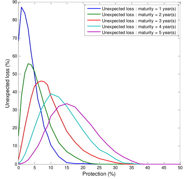
To show how the dispersion of capital varies as maturity increases, in Figure 2, we show the Unexpected Losses (ULs) for individual tranches plotted against their attachment points for different maturities. The ULs exhibit marked and increasing dispersion across the tranches as the maturity increases.
Here, we present calculations of capital based on the Ratings-based Monte Carlo approach and on the AFA inclusive of maturity adjustments as described in the last section.
The Ratings-based Monte Carlo model follows a ratings-based approach in which the ratings of individual loans evolve as correlated Markov chains. If there are J ratings categories, for a given initial rating, i, the M-period default probability equals the (i,J)th element in the M-fold product of the rating transition matrix.
The Ratings-based Monte Carlo model also includes risk-adjusted distributions for ratings transitions in that it is assumed that on a risk-adjusted basis, a given loan rating evolves also as a Markov chain with a time-homogeneous rating transition matrix. This latter matrix is derived (though a least square fitting technique) from a cross-section (i.e., values observed on a given date) of corporate bond spreads for different ratings and maturities.
In order to maintain consistency between the Ratings-based Monte Carlo model and the AFA, we derive the PDM not directly from an application of equation (3) but by taking for a rating i the (i,J) element of the product of the historical transition matrix employed in the Ratingsbased Monte Carlo model with the (M-1) fold product of the risk adjusted transition matrix also employed in the Ratings-based Monte Carlo model.[11]
To maintain capital neutrality as discussed above, the stressed default probability is calculated as: PDα,M = KIRB / LGD+ PDM (where KIRB is exclusive of Expected Losses) and the maturity adjustment for stressed ρiPool is given by equation (5) with ρ* = 1.0.
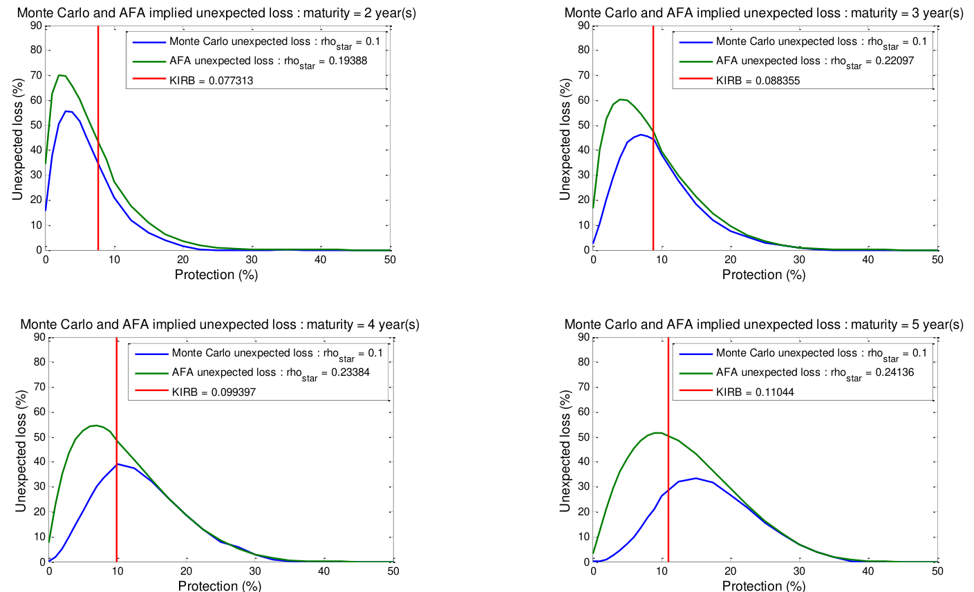
Table 4 and 5 show the total AFA capital calculated for BB and BBB-rated pools respectively. In each case, capital is shown for different maturities. The total capital equals KIRB as this approach is capital neutral. As explained above, the default probabilities, PM , are based on historical distributions for the first year and risk neutral distribution (extracted from spreads) for the subsequent M-1 periods. The tables show the implied stressed default probabilities that maintain capital neutrality, PDα,M .
Figure 3 presents the comparison of unexpected losses for thin tranches with a BB-rated underlying pool. Figure 3 shows the distribution of capital for different tranches using as default probability the combination of M-maturity historical and risk adjusted probabilities described above.
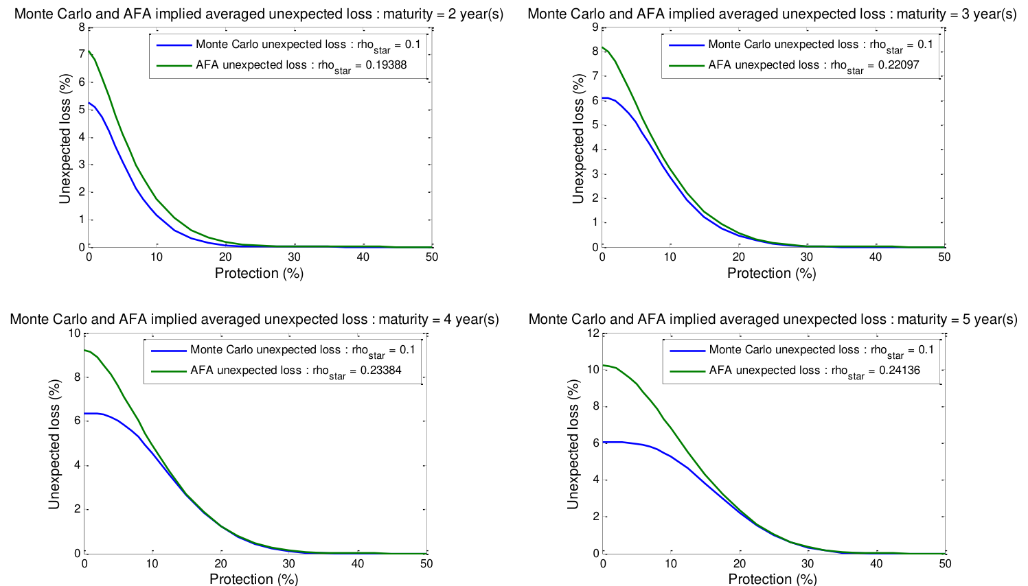
Figure 4 present the unexpected losses for senior tranches with attachment points equal to those of the thin tranches for which results are shown in Figure 3. These ‘senior tranche’ results are calculated by aggregating the capital for tranches to the right of any given attachment point. For any given attachment point, they, therefore, show the capital associated with a tranche from that point through to a detachment point equal to 100% of the par value.
Note that the discussion in this paper focusses primarily on corporate securitisations for which there is an explicit maturity adjustment in the Basel II IRBA rules. Retail lending under IRBA is not subject to maturity adjustment, however.
Apart from residential mortgages, this appropriately reflects the fact that such loans are generally short maturity. In the case of residential mortgages, the IRBA rules implicitly allow of maturity by adopting, in the capital charge formulae, an asset correlation parameter of 15% which is markedly higher than any empirical investigation of mortgage loan default is likely to yield.
In our view, it is helpful to maintain neutrality of on- and off-balance sheet loan holdings so we would not advocate the use of explicit maturity adjustments in the KIRB for mortgage loans. However, just as for corporate-loan-based securitisations, we believe the dispersion of capital across tranches should reflect maturity and hence we would suggest use of the boosted parameters described above.
SECTION 7 – RECONCILING AFA AND MC CAPITAL
From equation (13), it is apparent that capital from different models should be aligned so long as the hold-to-maturity loss distributions are aligned. The loss distributions should be calculated inclusive of a risk premium from periods 2 to maturity and conditional on a stress event affecting the bank’s wider portfolio.
In our calculations of capital, we obtain exact alignment of Monte Carlo and AFA-based capital calculations and reasonably close alignment for longer maturities. To examine the consistency of AFA and the Monte Carlo models, we may make two further adjustments.
First, the AFA calculations take as input KIRB , the on-balance sheet capital under Basel II rules. This capital includes a maturity adjustment in pool capital that does not necessarily agree with the impact of maturity on pool capital implied by the Ratings-based Monte Carlo model.
To adjust for this difference, we may use as input to the AFA the total pool capital implied by the Ratings-based Monte Carlo model. This may be achieved simply by using as stressed default probability, PDα,M , the following quantities: PDα,M =(MC UL+ MC EL/) LGD.
Second, the adjustment in correlations made in the AFA as described in the current paper comes from a simple multi-period Merton model. In this model, defaults only occur at the end of the maturity horizon. Ratings style models (and indeed genuinely multi-period Merton models) allow for defaults at intermediate points in time between the initial date and the final maturity.
It is well known among credit risk modellers that factor correlations behave differently in single- and multi-period models and that adjustments must be made to reconcile the two. The following steps are designed to effect reconciliation. Assuming a given correlation structure, we simulate a ratings-based Monte Carlo model with pairs of exposures until a final maturity. We then calculate the correlation of default events for those exposures and finally infer the asset correlation within a notional one-period model that would generate this degree of default correlation.
More precisely, to infer the correlations from MC simulated capital, consider two portfolios of M year exposures like the ones we are considering except suppose the recovery rate is zero and the par value is 1. Portfolio 1 consists of 2 BB-rated SPV pool exposures. Portfolio 2 consists of 2 BB-rated bank exposures. We calculate via a Monte Carlo the variances of the return on these two portfolios. We then infer from the following equations (for portfolios k=1,2) the pairwise correlations of loans in the pool with each other and with loans in the bank portfolio, denoted ρD1, and ρD,[2] .
Variance(Portfolio k) = 2 PDBB (1-PDBB ) + 2 ρD,k PDBB (1-PDBB ) for k =1,2 (21)
Here, PDBB is the M year cumulative default probability for a BB-rated loan. From these default correlations, one may infer the asset correlations: ρA,k , for k=1,2, using the fact that:
N[2] (PDBB,PDBB |ρA,k )− PDBB ρD,k = for k =1,2 (22) PDBB(1− PDBB )
Here, ρA1, is the correlation between pool exposures (ρPool) and ρA,[2] is the correlation
* between the bank exposures ( ρ). From the MC inferred ρPool and ρ, we can calculate ρ
* and ρM using the relations:
ρ − ρ * Pool ρ = 1− ρ (23) * ρ 1(− ρ) + (M −)1ρ * Pool ρM = 1− ρ+ M −1
The correlations inferred from MC capital after the adjustments just described are given in
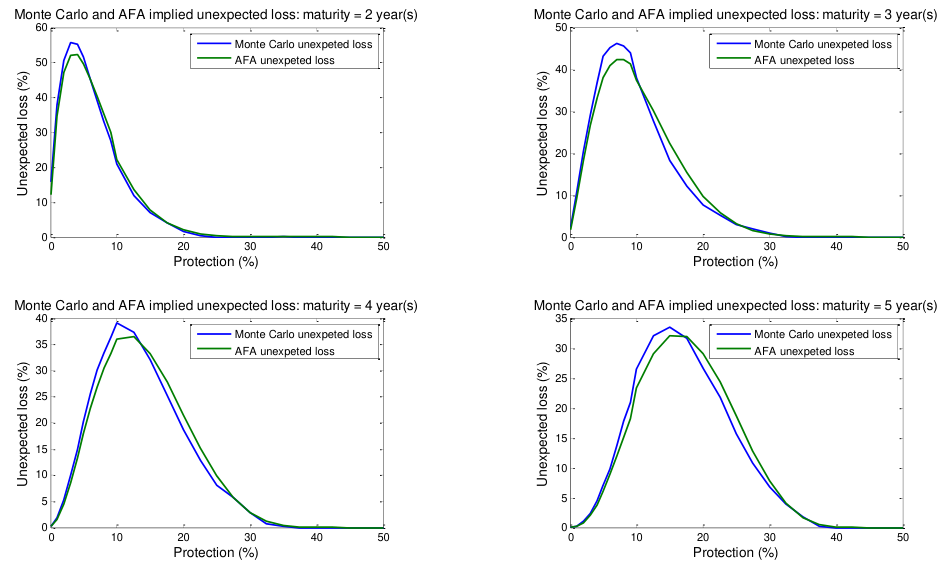
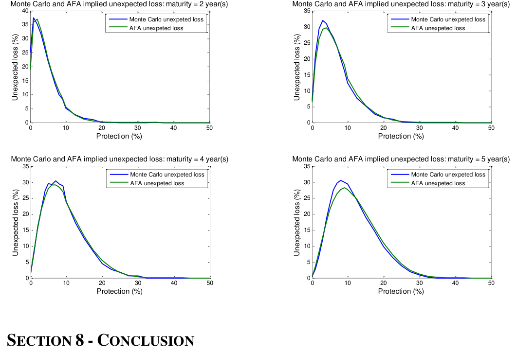
For comparison purposes, the correlation parameters used in AFA calculation are given in first adjustment described above of aligning total deal capital, we obtain the results as shown in Table 8 and Figures 5 and 6.[12] Figure 5 shows the comparisons between MC and AFA UL of thin tranches for a pool of BB-rated loans. Figure 6 shows the same comparisons for BBBrated pool assets.
Both Figures 5 and 6 show close correspondence between the AA and the Monte Carlo results. In other results base on CCC-rated pool assets, omitted to save space, a similar good correspondence was found.
This paper has analysed capital for securitisations for different maturities. In particular, we show how the total capital and the dispersion of capital across tranches of different seniorities is affected by maturity.
In the process, we have developed a rigorous, closed-form, multi-period model for securitisation capital and demonstrated that it is equivalent to the Arbitage Free Approach (AFA) of Duponcheele et al (2013a) with inputs adjusted for maturity. Our approach is fully consistent with both the AFA and the Simplified AFA (SAFA) proposed by Duponcheele et al (2013b).
Compared with the models proposed by the Basel Committee in its consultative document of December 2012 (BCBS (2012)), the model we propose has the important advantage of preserving neutrality of total securitisation capital with the IRBA capital charges required of a bank if it holds the pool exposures directly on balance sheet.
![Marginal VaRs for tranches (with BB-rated pool exposures)[9]](/api/media/file/fig-1588.png?prefix=media)
| Jarrow-Turnbull | Duffie-Singleton | |
|---|---|---|
| recovery MVaRs | recovery MVaRs | |
| Three- | Three- | |
| Homogeneous | year Six-year | year Six-year |
| Portfolio | maturity maturity | maturity maturity |
| Rating | loan loans | loans loans |
| AAA | 0.08 0.23 | 0.08 0.23 |
| AA | 0.31 0.77 | 0.29 0.85 |
| A | 0.55 1.33 | 0.54 1.41 |
| BBB | 3.65 4.43 | 3.39 4.76 |
| BB | 9.63 10.48 | 9.87 11.01 |
| B | 20.58 17.42 | 20.85 21.32 |
| CCC | 20.39 14.91 | 29.11 31.04 |
Notes: Portfolios consist of 500 exposures of equal face value and rating. VARs/MVaRs are calculated with a 99.9% confidence level and are measured in percent of the expected value at the 1-year VaR horizon. The correlation coefficient of the latent variables, ρ, equals 0.2. Under our assumptions, VaRs and MVaRs in percent of mean payoffs are identical.
| Percentage | Number of | |
|---|---|---|
| Category | of total par | tranches |
| Junior tranches | 10% | 10 |
| Mezzanine tranches | 40% | 16 |
| Senior tranches | 50% | 1 |
| Total | 100% | 27 |
| (B1) | IRBA (C1) | IRBA (D1) | MSFA | (D2) | MSFA | ||
|---|---|---|---|---|---|---|---|
| (A1) | MC | Capital | Capital Capital | (no | (A2) MC | Capital | (no |
| Maturity( Capital | for (exclude | EL) (include | EL) | caps or | Capital for (B2) | AFA caps | with |
| years) | pool | = AFA | = Kirb | floors) all | Tranches | Capital | floors) |
| BB-rated pool | exposures | ||||||
| 1 | 6.48% | 6.13% | 6.63% | 6.63% | 5.69% | 6.13% | 9.68% |
| 2 | 6.64% | 7.15% | 7.73% | 9.90% | 5.25% | 7.15% | 12.27% |
| 3 | 6.88% | 8.17% | 8.84% | 12.35% | 6.10% | 8.17% | 14.52% |
| 4 | 6.96% | 9.19% | 9.94% | 14.65% | 6.35% | 9.19% | 16.69% |
| 5 | 6.96% | 10.21% | 11.04% | 16.86% | 6.05% | 10.21% | 18.81% |
| BBB-rated pool | exposures | ||||||
| 1 | 3.04% | 2.75% | 2.86% | 2.86% | 2.76% | 2.75% | 5.36% |
| 2 | 3.20% | 3.53% | 3.68% | 4.38% | 2.56% | 3.53% | 6.85% |
| 3 | 3.51% | 4.32% | 4.49% | 5.60% | 3.12% | 4.32% | 8.17% |
| 4 | 3.92% | 5.11% | 5.31% | 6.80% | 4.02% | 5.11% | 9.50% |
| 5 | 4.39% | 5.89% | 6.13% | 8.04% | 4.57% | 5.89% | 10.84% |
Note: input data includes weekly averaged spreads by rating and maturity for US corporates for 2007 (source RCL) and Standard and Poor’s transition matrix (source: Standard & Poor’s (2007)).
| Maturity | PD | SPD | AFA UL Kirb(exclusive | EL) |
|---|---|---|---|---|
| historical PD | ||||
| 1 | 1.11% | 14.73% | 6.13% | 6.13% |
| 2 | 2.72% | 18.61% | 7.15% | 7.15% |
| 3 | 4.70% | 22.85% | 8.17% | 8.17% |
| 4 | 6.92% | 27.34% | 9.19% | 9.19% |
| 5 | 9.29% | 31.98% | 10.21% | 10.21% |
| one-year | historical PD + | risk adjusted PD | for 2, 3, 4 and 5 years | |
| 1 | 1.11% | 14.73% | 6.13% | 6.13% |
| 2 | 3.62% | 19.51% | 7.15% | 7.15% |
| 3 | 7.04% | 25.19% | 8.17% | 8.17% |
| 4 | 11.47% | 31.89% | 9.19% | 9.19% |
| 5 | 16.63% | 39.33% | 10.21% | 10.21% |
| Maturity | PD | SPD | AFA UL Kirb(exclusive | EL) |
|---|---|---|---|---|
| historical PD | ||||
| 1 | 0.25% | 6.35% | 2.75% | 2.75% |
| 2 | 0.61% | 8.46% | 3.53% | 3.53% |
| 3 | 1.08% | 10.68% | 4.32% | 4.32% |
| 4 | 1.66% | 13.01% | 5.11% | 5.11% |
| 5 | 2.34% | 15.43% | 5.89% | 5.89% |
| one-year | historical PD + | risk adjusted PD | for 2, 3, 4 and 5 years | |
| 1 | 0.25% | 6.35% | 2.75% | 2.75% |
| 2 | 2.09% | 9.94% | 3.53% | 3.53% |
| 3 | 4.03% | 13.63% | 4.32% | 4.32% |
| 4 | 6.15% | 17.50% | 5.11% | 5.11% |
| 5 | 8.52% | 21.61% | 5.89% | 5.89% |
| maturity rho_asset_p1 | rho_asset_p2 | rho_star rho_star_M | ||
|---|---|---|---|---|
| BB-rated | pool | |||
| 1 | 0.2693 | 0.1900 | 0.0979 | 0.0979 |
| 2 | 0.2267 | 0.1535 | 0.0866 | 0.1625 |
| 3 | 0.2104 | 0.1422 | 0.0796 | 0.1712 |
| 4 | 0.1963 | 0.1321 | 0.0739 | 0.1688 |
| 5 | 0.1871 | 0.1256 | 0.0704 | 0.1662 |
| BBB-rated | pool | |||
| 1 | 0.2798 | 0.2233 | 0.0727 | 0.0727 |
| 2 | 0.2506 | 0.1672 | 0.1002 | 0.1823 |
| 3 | 0.2428 | 0.1794 | 0.0773 | 0.1946 |
| 4 | 0.2225 | 0.1555 | 0.0794 | 0.1911 |
| 5 | 0.2164 | 0.1591 | 0.0682 | 0.1907 |
| rho_pool | rho rho_star | ||
|---|---|---|---|
| BB-rated pool | |||
| correlation | |||
| parameters | 0.27 | 0.1889 | 0.1 |
| BBB-rated pool | |||
| correlation | |||
| parameters | 0.3035 | 0.2261 | 0.1 |
| Maturity | MC UL | MC EL MC | capital | PD | SPD AFA | UL |
|---|---|---|---|---|---|---|
| BB-rated | pool | |||||
| 1 | 0.0569 | 0.0050 | 0.0619 | 0.0111 | 0.1376 | 0.0569 |
| 2 | 0.0525 | 0.0323 | 0.0849 | 0.0718 | 0.1887 | 0.0525 |
| 3 | 0.0610 | 0.0684 | 0.1294 | 0.1520 | 0.2876 | 0.0610 |
| 4 | 0.0635 | 0.1106 | 0.1741 | 0.2458 | 0.3869 | 0.0635 |
| 5 | 0.0605 | 0.1543 | 0.2148 | 0.3429 | 0.4773 | 0.0605 |
| BBB-rated | pool | |||||
| 1 | 0.0276 | 0.0011 | 0.0287 | 0.0025 | 0.0638 | 0.0276 |
| 2 | 0.0256 | 0.0241 | 0.0497 | 0.0536 | 0.1104 | 0.0256 |
| 3 | 0.0312 | 0.0470 | 0.0782 | 0.1043 | 0.1737 | 0.0312 |
| 4 | 0.0402 | 0.0705 | 0.1106 | 0.1566 | 0.2459 | 0.0402 |
| 5 | 0.0457 | 0.0946 | 0.1404 | 0.2103 | 0.3119 | 0.0457 |
Note: here, MC capital = MC UL + MC EL
References
Basel Committee on Bank Supervision (2001) “Treatment of Asset Securitisation,” Bank for International Settlements, BCBS Working Paper 10, October.
Basel Committee on Bank Supervision (2002) “Second Working Paper on Securitisation,” Bank for International Settlements, BCBS Working Paper 11, October.
Basel Committee on Bank Supervision (2006) “Basel II: International Convergence of Capital Measurement and Capital Standards: A Revised Framework - Comprehensive Version,” Bank for International Settlements, BCBS No.128, June.
Basel Committee on Bank Supervision (2009) “Enhancements to the Basel II framework,” Bank for International Settlements, BCBS No.157, July.
Basel Committee on Bank Supervision (2012) “Revisions to the Basel Securitisation Framework,” Bank for International Settlements, BCBS No.236, December.
Basel Committee on Bank Supervision (2013a) “Foundations of the Proposed Modified Supervisory Formula Approach,” Bank for International Settlements, Working Paper 22, January.
Basel Committee on Bank Supervision (2013b) “The Proposed Revised Ratings-Based Approach,” Bank for International Settlements, Working Paper 23, January.
Black, Fischer and John Cox (1976) “Valuing Corporate Securities: Some Effects of Bond Indenture Provisions,” Journal of Finance, Vol. 31, pp. 351-67.
Bohn, Jeffrey R., (2000) “An Empirical Assessment of a Simple Contingent-Claims Model for the Valuation of Risky Debt,” Journal of Risk Finance, Summer, pp. 55-77.
Duffie Darrell and Kenneth J. Singleton (1999) “Modeling term structures of defaultable bonds,” Review of Financial Studies, Vol. 12, pp. 687-720.
Duponcheele, Georges, William Perraudin and Daniel Totouom-Tangho (2013a) “A Principles-Based Approach to Regulatory Capital for Securitisations,” BNP-Paribas mimeo, April.
Duponcheele, Georges, William Perraudin and Daniel Totouom-Tangho (2013b) “The Simplified Arbitrage-Free Approach: Calculating Securitisation Capital based on Risk Weights Alone,” BNP-Paribas mimeo, July.
Duponcheele, Georges, William Perraudin, Alastair Pickett and Daniel Totouom-Tangho
(2013) “Granularity, Heterogeneity and Securitisation Capital,” BNP-Paribas mimeo, August.
Gourieroux, Christian, J. P. Laurent, and Olivier Scaillet (2000) “Sensitivity Analysis of Values at Risk,” Journal of Empirical Finance, 7, 225–245.
JP Morgan (1997) “Creditmetrics – technical document,” Discussion paper, JP Morgan, New York.
Kiesel, Rudiger, William Perraudin and Alex P. Taylor (2003) “The Structure of Credit Risk: Spread Volatility and Ratings Transitions,” Journal of Risk, Vol. 6, No. 1, Fall, pp. 1-37.
Jarrow Robert A. and Stuart M. Turnbull (1995) “Pricing derivatives on financial securities subject to credit risk,” Journal of Finance, Vol. 50, pp. 53-86.
Jarrow Robert A., David Lando and Stuart M. Turnbull (1997) “A Markov model for the term structure of credit risk spreads,” Review of Financial Studies, Vol. 10, No. 2, pp. 481-523.
Lamb, Robert, Vladislav Peretyatkin and William Perraudin (2005) “Hedging and Asset Allocation for Structured Products,” RCL mimeo.
Longstaff, Francis A. and Eduardo S. Schwartz (2001) “Valuing American Options by Simulation: A Least-Squares Approach,” Review of Financial Studies, Vol 14, No. 1, pp.113- 147.
Merton, Robert C., (1974) “On the Pricing of Corporate Debt: The Risk Structure of Interest Rates,” Journal of Finance, Vol. 29, pp. 449-70.
Peretyatkin, Vladislav and William Perraudin (2004) “Capital for Structured Products,” Risk Control Limited.
Standard and Poor’s (2008) “Default, Transition, and Recovery: 2007 Annual Global Corporate Default Study and Rating Transitions (Premium),” February.
Vasicek, Oldrich (2002) “The Distribution of Loan Portfolio Value,” Risk, December.
Appendix 1: statistical data inputs
Table A1: RCL all obligor spreads (2007 April – June) 1 2 3 4 5
AAA 0.338 0.373 0.408 0.444 0.481 AA 0.467 0.495 0.531 0.569 0.610 A 0.530 0.586 0.635 0.683 0.732 BBB 0.920 0.932 0.963 1.010 1.070 BB 1.213 1.445 1.728 1.999 2.233 B 1.880 2.480 2.869 3.119 3.273 CCC 4.963 4.828 4.694 4.561 4.430 Source: RCL calculations. Spreads are shown in percent by rating and maturity in years.
Table A2: Rating transition probabilities extracted from S&P data 1981-2007 AAA AA A BBB BB B Cs default AAA 91.39% 7.95% 0.47% 0.09% 0.09% 0.00% 0.00% 0.00% AA 0.62% 90.99% 7.62% 0.56% 0.06% 0.10% 0.02% 0.01% A 0.04% 2.17% 91.49% 5.62% 0.41% 0.17% 0.03% 0.06% BBB 0.01% 0.18% 4.24% 90.07% 4.31% 0.77% 0.17% 0.25% BB 0.02% 0.06% 0.23% 5.90% 83.88% 7.93% 0.87% 1.11% B 0.00% 0.06% 0.18% 0.32% 6.73% 83.01% 4.50% 5.20% Cs 0.00% 0.00% 0.28% 0.42% 1.18% 13.60% 54.88% 29.64% default 0.00% 0.00% 0.00% 0.00% 0.00% 0.00% 0.00% 100.00% Source: Standard and Poor’s (2008).
Table A3: Spreads Reverse Engineered from the MSFA Formula 1 2 3 4 5 AAA 0.005 0.140 0.400 0.650 0.848 AA 0.019 0.278 0.635 0.922 1.124 A 0.036 0.388 0.796 1.094 1.291 BBB 0.114 0.696 1.181 1.475 1.641 BB 0.373 1.272 1.768 1.993 2.081 B 1.565 2.670 2.911 2.887 2.782 CCC 9.118 7.467 6.194 5.296 4.638 Source: the author’s calculations. Spreads are shown in percent by rating and maturity in years.
Appendix 2: ratings-based modelling methodology
Individual Exposures and Their Ratings Histories
In this section, we describe our approach to simulating dependent changes in the credit quality of simple exposures like bonds and loans. The exposition follows that of Lamb, Peretyatkin and Perraudin (2005). Consider a set of I such exposures denoted i=1,2,..,I. Suppose that, at date t, exposure i has a rating, Rit, which can take one of K values, 1,2,…,K. Here, K corresponds to default, while state 1 indicates the highest credit quality category.
Since we wish both to price and to study the dynamics of ratings, we must distinguish between actual and riskadjusted distributions of ratings changes. Assume that under both actual and risk-adjusted probability measures, the rating Rit evolves as a time-homogeneous Markov chain.
The actual and risk-adjusted K × K transition matrices are denoted: M and M* respectively. The ,(i j) -
* * * elements of M and M are mi,j and mi, j respectively. Let mi, j,τ and mi,j,τ denote the ,(i j) -elements of the * τ * τ-fold products of the matrices M and M , i.e., M and (M )τ.
The actual transition matrix, M may be estimated from historical data on bond ratings transitions. We employ as our estimate the Standard and Poor's historical, all-issuer transition matrices for the relevant sample period.
* The risk-adjusted transition matrix M may be deduced from bond market prices, in particular, from spread data on notional pure discount bonds with given ratings. To see how one may achieve this, note that if credit risk and interest rate risk are independent and spreads only reflect credit risk (i.e., there are no tax or liquidity (i) effects), the τ-maturity spread on a pure discount bond with initial rating i, denoted Sτ , satisfies:
(i) * * exp(− Sτ τ) = mi,K,τ γ + (1− mi,K,τ ) (A1) Here, γ is the expected recovery rate in the event of default.
Let T ≡τ[1],τ[2],...,τd denote a set of integer-year maturities. To infer the risk-adjusted matrix, we may choose
* for i, j =2,1,...,K −1 and τ∈T to minimize: mi, j
K−1
(i) * * (A2) exp − S τ − m γ + 1− m ( [ τ ] ( i,K,τ ( i,K,τ ) ∑∑ minmi*,j τ∈T i=1
* * Here, note that the mi,K,τare implicitly functions of the mi, j .[13]
In performing this calculation, we assume that the recovery rate γ is 50% and that the maturities in are 1, 2, 3, 4, 5, 6, 7, and 8 years. The spread data we employ are time averages of pure discount bond spreads calculated by Bloomberg based on price quotes for bonds of different ratings and maturities issued by industrial borrowers (see Table 2). The risk-adjusted transition matrix obtained in this way is given in Table 1.
Bond Ratings Histories and Values
The last section describes a theoretically consistent set of actual and risk-adjusted distributions governing the dynamics of ratings for our set of I exposures. Now consider how one may simulate changes in ratings building in dependence between ratings changes for different obligors.
We employ the ordered probit approach widely used in ratings-based portfolio credit risk models. For any row of M (say the jth row), one may deduce a set of cutoff points Z j,k for k=1,2,…,K-1 by recursively solving the equations:
mj1, = Φ(Z j1,) mj,[2] = Φ(Z j,[2]) − Φ(Z j1,) (A3)

mj,K = 1− Φ(Z j,K−[1]) Here, Φ(.) is the standard normal cumulative distribution function. Doing this, we obtain a set of ordered cut off points Z j1, ≤ Z j,[2] ≤ ... ≤ Z j,K−[1].
Given an initial rating j, to simulate a change in the rating from t to t+1 for exposure i, we draw a random variable Xi,t+[1]. If Z j,k−[1] < Xi,t+[1] ≤ Z j,k (where by convention Z j1, = −∞ and Z j,K = ∞ ), exposure i's rating at t+1 is k.
The latent variables Xi,t that determine changes in ratings are assumed to be standard normal random variables. To include dependency between the ratings changes of different exposures, assume that the Xi,t , for the exposures i=1,2,…,I, possess a factor structure, in that: J Xi,t = 1− βi ∑αi,j f j,t + βi εi,t (A4) j=1 Here, the f j,t are factors common to the latent variables associated with the different credit exposures and the are idiosyncratic shocks. The are standard normal and the weights are chosen so that εi,t f j,t and the εi,t αi,j the sum over j of the factor components, αi,j f j,t , is also standard normal. Note that, in our implementation of this approach for the evaluation of Monte Carlo-based capital as described in the main body of the paper, we choose theαi, j andβi parameters to replicate the factor structure of the AFA model.
If one knows the risk-adjusted probabilities of default for individual exposures and assumes that defaults, recovery rates and shocks to interest rates are independent, the valuation of individual exposures at some future date conditional on ratings is straightforward. For example, under these assumptions, the price Vt,R of a defaultable fixed rate bond with initial rating R, coupons c, and principal Q is: N * * * * Vt,R =∑c exp(− rt,t+i i ) (1− mR,K,i ) + γ mR,K,i ) +Q exp(− rt,t+N N )(1− mR,K,N ) + γ mR,K,N ) i=[1] (A5) Here, rt,t+i is the i-period interest rate at date t. It is simple to derive pricing expressions for floating rate loans and many other exposures including Credit Default Swaps (CDS), guarantees, letters of credit etc, under these assumptions as well.
Drawing together the various elements described above, one may simulate dependent ratings histories for all I exposures. The steps involved are:
1. Draw the f.,t and εi,t and calculate the latent variables for each exposure and each period using equation (A4).
2. Deduce the time path followed by the ratings by comparing the latent variable realizations with the cutoff point intervals Z j,k−[1] < Xi,t+[1] ≤ Z j,k .
3. Conditional on the rating at the chosen future date, price the I exposures.
4. Repeat the exercise many times to build up a data set of value and rating realizations.
Conditional Pricing Functions
The payoff on a structured exposure depends in a complex way on the performance of the pool of underlying exposures, typically bonds or loans. It is apparent from the above how one may simulate the values of the individual exposures in the pool. To analyze risk for a structured exposure, however, one must be able to simulate its price which is clearly much more complicated.
To put the task in context, one might consider simulating the underlying exposures up to the horizon of interest and then by simulating repeatedly from that date on, price the exposure at the VaR horizon through a Monte Carlo. This effectively amounts to performing a pricing Monte Carlo for each replication of the initial Monte Carlo. But, this approach is clearly infeasible however since it is computationally too costly.
Our alternative approach, which is much more efficient computationally, consists of performing an initial valuation Monte Carlo (denoted Monte Carlo 1) that serves to estimate conditional pricing functions. These pricing functions are then used in a second risk management Monte Carlo (denoted Monte Carlo 2) in which we deduce risk measures like Value at Risk.
To describe more precisely Monte Carlo 1 and the pricing functions it yields, consider, as before, a set of credit exposures, i=1,2,…,I with ratings histories Ri,t for t=0,1,…,T where T is the maturity date of the CDO.
For a given structure, we define the cash flow waterfall to be a set of rules that, conditional on the evolution of ratings Ri,t , determine the cash flows for t=0,1,…,T and i=1,2,…,I for each tranche in the structure.[14]
The waterfall rules may be described formally by a set of functions for dates t=0,1,2,…,T that map the ratings histories up to t into cash flows on the individual tranches, j=1,2,…,J, at that date:
cj,t = Fj,t ({Ri,τ;τ= 2,1,0,...,t;i =2,1,..., I}) (A6)
To estimate the pricing functions, we follow the steps:
1. Simulate correlated ratings histories starting from the initial values at t=0 to the terminal date T. This simulation is performed using the ordered probit method described above but with the risk adjusted transition matrix, M*, rather than the actual matrix, M.
(m)
2. Repeat the simulation M times. If c j,t is the cash flow in period t on tranche j in the mth simulation, we can define the summed discounted cash flow at date t[1] (where 0 < t[1] < T ) on tranche j and for (m) replication m, denoted DCFt, j,t[1] , as: T
(m) (m) (A7) DCFt,j,t[1] = ∑ cj,i Pt,t[1],i i=t[1]+1 Here, Pt,t[1],i is the forward discount factor at date t for discounting a cash flow at date i back to date t[1] . (m) The quantity DCFt, j,t[1] in the above equation is the cash flow on a given tranche from s onwards discounted back to that date using forward interest rates implied by the term structure at the initial date t.
3. We wish to obtain pricing functions for the tranches conditional on information at date t[1] . To represent (m) that information, we define a set of S statistics ht[1],s (indexed s=1,2,…,S) of the individual obligor ratings Ri,τ up to the datet[1] :
(m) ht[1],s = Ht[1],s ({Ri,τ;τ= 1,0,...,t;i =2,1,...,I}) s =2,1,...,S (A8)
The superscript m shows that statistic s is observed in simulation m. In principal, there are many variables observable at t[1] that one might expect would affect cash flows on the tranches subsequent to that date. A good example is the fraction of pool value in each of the rating categories at date t[1] . Such fractions are likely to be associated with systematically high or low outcomes for the subsequent cash flows on the tranches.
(m)
4. To derive a pricing function, we regress the discounted, summed cash flows DCFt, j,t[1] on the (m) information variables, ht[1],s . (The regression function we employ is more complicated than a simple linear regression. We discuss the regression we use in the next subsection.)
To understand why this yields a pricing function, suppose that t[1] = 0 and one performed a simple linear regression on a unit constant. This would be the same as averaging the discounted cash flows (m) over m. Given that the simulations have been performed using risk neutral distributions, this DCFt, j,t[1] would yield an estimate of the price of the tranche at date 0 since we would simply be conducting a risk neutral Monte Carlo valuation of the claim.
By regressing the discounted summed cash flows, simulated using risk neutral distributions on the information variables, we obtain a conditional pricing model. Evaluating the regression function at given levels of the information variables yields the prices of the tranche when the information variables take the values specified.
Estimating Conditional Prices
We described above how we derive a conditional pricing function by regressing the summed, discounted cash flows on the information variables but were unspecific about what form the regression should take. In this subsection, we discuss for the form of the regression that it is advisable given the nature of payoffs on tranches.
In general, the regression model one employs should reflect the stochastic behavior of discounted payoffs on that tranche. Consider the density of discounted payoffs on a given tranche. A low credit quality tranche is likely to have an atom of probability associated with a zero payoff. A very senior tranche may have an atom associated with full repayment (although even a senior tranche may have a state dependent payoff if poor performance of the pool triggers early substantial amortization). A mezzanine tranche may have atoms associated with zero payoffs and another associated with full repayment.
In light of this, we use different regression functions for different tranches depending on the number of replications in the Monte Carlo 1 for which the tranche in question either (a) defaults or (b) returns a zero discounted payoff. We say that a tranche “defaults” if it pays less than the maximum contractual amount by the maturity date of the structure. (If a coupon payment is missed before this maturity date, the unpaid coupon is added to principal. A tranche is said to default if the full principal including unpaid coupons added to principal during the life of the structure cannot be fully paid at the maturity date.)
To be specific, a tranche is allocated to one of the following types of regressions depending upon its default behavior.
1. Equity Tranche: A tranche is treated as an equity tranche if it is the most junior tranche in the structure or if it defaults more than0.5% of the time. Equity tranches are valued using a linear regression of the discounted future payoff on the state variables. So the valuation expression is: Equity value = Xtβ (A9) Here, β is a vector of regression coefficients and X t is a row vector of state variables.
2. Senior Mezzanine Variable Tranche: A tranche is treated as a mezzanine variable tranche if it defaults more than 0.05% of the time and more than 10% of payoffs observations in the Monte Carlo differ from the payoff in the previous replication. The pricing expression is: exp(X 'β[1]) 1 Senior mezzaninevariablevalue= Xtβ[2] + dt Xtβ[3] 1+ exp(X 'β[1]) 1+ exp(X 'β[1]) (A10) Here, β[1] is a vector parameter values for a logit model of the dummy variable that, for a given Monte Carlo replication, equals unity if the tranche defaults in the sense that it has a zero discounted payoff and otherwise is zero. The logit model is estimated by Maximum Likelihood. Xtβ[2] is the fitted value from an ordinary least squares regression of the discounted tranche payoffs on the state variables, X t , conditional on a default (in the sense just given) having occurred. dt Xtβ[3] is the fitted value from a linear regression of the discounted tranche payoffs on dt Xt conditional on no default where dt is the outstanding par at the time of valuation.
3. Senior Mezzanine Constant Tranche: A tranche is treated as a mezzanine variable tranche if it defaults more than 0.05% of the time and less than 10% of payoffs observations in the Monte Carlo differ from the payoff in the previous replication. The pricing expression is: exp(X 'β[1]) 1 Mezzaninevariablevalue= Xtβ[2] +β,3[0] 1+ exp(X 'β[1]) 1+ exp(X 'β[1]) (A11) Here, β[1] is a vector parameter values for a logit model of the dummy variable that, for a given Monte Carlo replication, equals unity if the tranche defaults in the sense that it has a zero discounted payoff and otherwise is zero. The logit model is estimated by Maximum Likelihood. Xtβ[2] is the fitted value from an ordinary least squares regression of the discounted tranche payoffs on the state variables, X t , conditional on a default having occurred. β,3[0] is mean of the discounted tranche payoffs conditional on no default.
4. Senior Variable Tranche: A tranche is treated as senior variable if it defaults less than 0.05% of the time and discounted payoffs in successive Monte Carlo replications differ more than 10% of the time. Such tranches are valued as: Senior variablevalue = dt Xtβ (A12) Here, dt Xtβis the fitted value from a regression of the discounted payoff on dt Xt .
5. Senior Constant Tranche: A tranche is treated as senior constant if it defaults less than 0.05% of the time and discounted payoffs in successive Monte Carlo replications differ on fewer than 10% of occasions. Such tranches are valued as: Senior variablevalue = β[0] (A13) Here, β[0] is the mean discounted payoff.
An important issue is: what “state”' or ``explanatory'' variables should be included in the statistical pricing (m) models? Examples of statistics that one may sensibly choose for the Sk,t[1] are the fractions of the value of the pool in different rating categories and interest rate levels for different maturities and exchange rates. If the model is simulated without interest and exchange rate risk, then the ratings fractions alone may be used.
Appendix 3: maturity and concentration correlation
A3-1 Brownian and Gaussian variables with the concentration correlation
The credit quality of individual loans is driven by latent variables describing the underlying values of the borrowers’ assets, . We suppose that:
(A3.1) √ √ √ √ √
Here, , , are the levels of standard Brownian motions (with , , all equal to zero) and, hence, have discrete time increments that are normally distributed and serially independent. is the single common factor driving the credit quality of the bank’s wider portfolio while is another common factor orthogonal to . is a factor idiosyncratic to the ith borrower.
The ith loan defaults if the Gaussian latent variable falls below a threshold level . The probability of default of the ith loan at maturity is then given by:
![Equation: cM PDM = Ρ[Zi,M < −cM ]= N − (A3.2)](/api/media/file/eq-146-300x24.png?prefix=media)
M
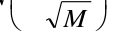
Here, N(.) is the cumulative density function of a standard normal distribution.
A3-2 Portfolio losses conditional on factors
Like Vasicek (2002), consider a homogeneous portfolio of loans in equal size and loss-givendefault . Then, the total loss on the portfolio assuming a par value of unity is defined by:
n n LGD LGD L = ∑i=1Li = ∑i=11{Zi,M <−cM } (A3.3) n n
Here, { } is the indicator function.
The portfolio loss when par value is unity, conditional on and , is given by:
n (A3.4) L(YB,M , XM ) = L | YB,M , XM = LGD⋅ ∑i=[1]1{Zi,M<−cM|YB,M ,XM} ≅ LGD⋅Ρ(Zi,M < −cM | YB,M , XM ) n
From (A3.1), we can have that:
*
![Equation: − cM − ρYB,M − 1− ρ ρ XM Ρ[Zi,M < −cM |YB,M , XM ]= Ρ εi,M < * 1− ρ 1− ρ](/api/media/file/eq-148-300x40.png?prefix=media)
Y

− − ρ − 1− ρ ρ

* M

Y

M M

= N *

1− ρ 1− ρ

In summary, the total portfolio loss when par value equals unity, conditional on and , is given by: Y
![Equation: −1 B,M * X M N (PDM ) − ρ − 1− ρ ρ M M (A3.6) L(YB,M , X M ) = LGD⋅ Ρ[Zi,M < −cM |YB,M , X M ]= LGD⋅ N *](/api/media/file/eq-156-300x27.png?prefix=media)
1− ρ 1− ρ

A3-3 Portfolio losses conditional on factors
In what follows, we shall wish to condition on a stress event affecting the bank’s portfolio factor in the period from 0 to date . This motivates an adjustment in the conditioning just described. Suppose that the maturity date of the loan exceeds the VaR horizon . In Basel regulations this horizon is one year ( ).
, we can By splitting the level of the Brownian motion at date as follows:YB,M = YB,H +YB,M −YB,H rewrite equation (A3.6) as:
−1 *

M 1− ρ 1− ρ

(A3.7) −1 *

= LGD⋅ N *

M 1− ρ 1− ρ

By defining as a standard normal Gaussian random variable, in law, we have the following relation:
* * ρ(YB,M −YB,H ) + 1−ρ ρ XM ≅ (M − H)ρ+ M 1(−ρ)ρW (A3.8)
L(YB,M , XM ) ≅ L(H, M )(Y,W )
−1 *

= LGD⋅ N *

M 1− ρ 1− ρ

A3-4 Value at Risk of the portfolio loss: ( )
The Marginal Value at Risk of the portfolio at the bank’s -quantile is the expectation of the −1 = N (α) conditional loss at a confidence interval of YB1, :
−1 MVaRα(H, M ) = Ε[L(H, M )(Y,W |)YB1, = N (α)]
−1 −1 *

= LGD⋅ Ε N *

( ( ))√ √ ( ) By defining ( ) and ( ) √( ) ( ) , we can √ ( )( ) √ ( )( ) simplify to: (A3.11) ( ) [ ( ( ) ( ) )]
Using the property of Gaussian random variables: [ ( )] ( √ ), we have:

−1 −1

N (PDM ) M − ρ H N (α)

*
![Equation: M 1− ρ 1− ρ MVaRα(H, M ) = LGD⋅ N [2]](/api/media/file/eq-171-300x28.png?prefix=media)
*

1+ − *

−1 −1

= LGD⋅ N (A3.12)

(M − H )ρ+ M 1(− ρ)

M

= LGD⋅ N

1− ρ

M

A3-5 Stressed portfolio losses conditional on the factor:
Define the stressed default probability at horizon as PDα,M . This represents probability of default
−1 of an individual pool asset conditional on the bank stress event, YB1, = N (α) .
MVaRα(H,M ) PDα,M = (A3.13) LGD
From line 2 of equation (A3.12), we have the result that:
MVaR (H, M )

LGD

−1 = N (PDα,M ) (M − H)ρ+ M 1(− ρ)
The stressed portfolio loss conditional on the factor W becomes: −1 L(W | YB,H = N (α))
−1 *

= LGD⋅ N *

M 1(− ρ)(1− ρ )

*
− (M − H )ρ+ M 1(− ρ)ρ W](/api/media/file/eq-186-300x39.png?prefix=media)
(A3.15)

* (M − H )ρ+ M 1(− ρ)ρ

1−

(M − H )ρ+ M 1(− ρ)

−1

= LGD⋅ N

1− sρ(H, M )

Since W is Gaussian, one may obtain a distribution function for losses with the appropriate conditioning on the bank stress event by inverting the last equation to obtain W as a function of L and then substitute this function of L in the standard Gaussian cumulative distribution function.
The stressed pairwise correlation between exposures in the pool is:
* (M − H)ρ+ M 1(− ρ)ρ (A3.16) sρ(H,M ) = M − Hρ
When the VaR horizon is one period ( ), the stressed correlation is:
* * (M −)1ρ+ M 1(− ρ)ρ M (ρ+ 1(− ρ)ρ) − ρ * ρM = sρ,1( M ) = = M − ρ M − ρ (A3.17) * Mρpool − ρ (M −)1ρpool + 1(− ρ)ρ = = M − ρ (M −)1 + 1(− ρ)
* * . This is the result obtained in Duponcheele et ρ = ρ Here, ( ) . When , M * al (2013a) for the Basel VaR horizon of unity. When , ρM ≈ ρpool.
Notes
[1] Dr. Georges Duponcheele is Head of Banking Solutions, BNP Paribas. Dr. William Perraudin is Director of RCL and Adjunct Professor of Imperial College, London. Dr. Daniel Totouom-Tangho is in Credit Quantitative Research, BNP Paribas and Adjunct Associate Professor of Financial Engineering at New-York University (NYU- Poly). Correspondence should be addressed to the authors at georges.duponcheele@bnpparibas.com, william.perraudin@riskcontrollimited.com or daniel.totouom-tangho@bnpparibas.com.
[2] The authors thank from BNP Paribas, Fabrice Susini, Antoine Chausson, Duc Dam Hieu, Alexandre Linden, Paul Vercoustre and from other institutions Alexander Batchvarov, Shalom Benaim, Stephan Meili and Alastair Pickett for their contribution, their numerous and helpful comments. William Perraudin thanks Peng Yang for excellent research assistance and many insightful comments and suggestions. Totouom-Tangho thanks Kaiwen Xu for ensuring that time was made available to develop this solution. All errors are ours. The views expressed are the authors’ own and not necessarily those of BNP Paribas nor those with whom we had discussions or their firms.
[3] This has lead one major regulator to limit use of the SFA by banks it regulates.
[4] This approach was suggested to us by Shalom Benaim whom we also thank for stressing the importance of maturity effects in the dispersion of capital across tranches.
[5] This parameter could be set through calibration using the fact that expected losses implicit in bond market spreads represent expected losses plus a risk premium. In a similar fashion, BCBS (2013a) bases a calibration of a risk premium parameter used in the MSFA on a study by Bohn (2000).
[6] Three approaches are commonly employed in portfolio credit risk models for handling recoveries. In each case, recoveries are assumed to equal a fractional recovery rate applied to a scale variable. Jarrow and Turnbull (1995) and Jarrow, Lando and Turnbull (1997) take the scale variable to equal the value at default of a default free bond or loan with the same contractual cash-flows as the defaulted security. Duffie and Singleton (1999) assume the scale variable is the value of the bond or loan immediately prior to default. If the bond was rated lowly, say at CCC just before default, one may see that the implied recovery will be lower than under the Jarrow-Turnbull assumption. The difference in a practical modelling exercise is less great than it might seem in that the fractional recovery rate employed may be adjusted depending on the scale variable approach employed, or, to put it another way, different data may be employed in calibrating the recovery rate. A third possible approach is to use as scale variable the par value of the loan or bond.
[7] One might expect that entitlement in bankruptcy settlements will be based on par values rather than default free securities or value prior to default which argues in favour of using par value.
[8] Note that, in each case, both the pool assets and the securitisation notes are presumed to have the same maturity.
[9] In interpreting the figure, note that the MVaRs are plotted vertically above their attachment points and that both Monte Carlo and AFA calculations of MVaRs make explicit allowance for the fact that the tranches are discretely thick in that both attachment and detachment points are taken account of in calculating the risk statistics.
[10] Clearly, when implemented for a 1-period horizon, the two models are identical mathematically so that the only source of discrepancy between the capital implied by the two is sampling error in the Monte Carlo. Figure
[1] is therefore reassuring that the two models are correctly aligned and illustrates the extent of the sampling error in a Monte Carlo with 5 million replications.
[11] This approach is consistent with the requirements of equation (13, that one employ distributions based on historical distributions in the first period and distributions inclusive of risk premiums in subsequent periods. *
[12] Here, AFA UL is calculated by substituting the MC implied PD, SPD, ρPool and ρM into the AFA formula.
[13] Note that in performing the optimisation, we attach penalties to the objective function if entries in the transition matrix become negative in the course of minimisation. This ensures the resulting risk-adjusted matrix is well-behaved.
[14] The cash flows may depend on a set of K other state variables (for example, interest rates or exchange rates) that we denote S(k,t)for k=1,2,…,K. The may be introduced into the pricing functions without problem but we omit them here to simplify the notation.