

This study examines whether capital charges for infrastructure debt should be lower than the charges currently required by the Solvency II and IAIS regulatory frameworks. This question is important as (i) infrastructure investment is widely viewed as a key component of economic development and (ii) historical data on infrastructure debt strongly suggests that this class of corporate debt is much less risky than, for example, corporate bonds.
Executive Summary
This study examines whether capital charges for infrastructure debt should be lower than the charges currently required by the Solvency II and IAIS regulatory frameworks. This question is important as (i) infrastructure investment is widely viewed as a key component of economic development and (ii) historical data on infrastructure debt strongly suggests that this class of corporate debt is much less risky than, for example, corporate bonds.
The European Authorities regarded the issue as so important that they reopened the calibration of the Solvency II charges late in the development of that framework and adopted somewhat lower charges for a restricted category of infrastructure debt. So far, the IAIS in developing its International Capital Standard (ICS) has not made any concession to the low credit risk nature of infrastructure loans.
This report revisits the calibration of Solvency II and the ICS, deducing capital charges for credit exposures with the superior credit performance of infrastructure loans. The calibration approaches adopted are designed to be as close possible in spirit and approach to those apparently used by the regulatory authorities (EIOPA in the case of Solvency II and the IAIS in the case of the ICS).
For the ICS charges, we perform a bottom up calibration using variants of the modelling approach (based on a well-known paper by Vasicek (2001)). For the Solvency II charges, we suppose that the current framework is correctly calibrated for corporate bond claims and then calculate what would be appropriate capital charges for other debt claims that have the historical credit performance observed for different categories of infrastructure loans. In both analyses, we build on past work by Jobst (2018) who studies infrastructure risk and capital charges in some detail.
An important aspect of the Solvency II capital charges is that they include a diversification adjustment that is specific to the balance sheet of the insurer performing the calculation. We calculate capital charges (i) for a purely specialist insurer only holding corporate debt and (ii) for a typical European life insurer with a balance sheet investigated in past studies by us and other authors (see Höring (2012) and Kutas, Perraudin and Qiu (2016)).
The key findings of our study are as follows.
• Both before and after diversification adjustments, Solvency II capital charges for infrastructure are about a third higher than is justified by a careful recalibration consistent with the methods of the EIOPA approaches.
• This statement is true both for High Income Country (HIC) and Medium and Low-Income Country (MIC/LIC) infrastructure loans.
• Applying the IAIS approaches to capital charge calibrations using historical default probability and recovery data, one obtains charges for infrastructure loans that are between two thirds and three quarters lower than those included in the ICS (depending on the calibration methodology employed).
• The big difference between current ICS charges and those merited by infrastructure loans is explained by assumptions about Loss Given Default (LGD) rates which are much lower for infrastructure loans than for most corporate debt claims.
• Historical data show that infrastructure loans originated in MIC/LICs exhibit a credit performance that is no worse than that of infrastructure loans originated in HICs.
• Hence, there is no justification in regulatory frameworks to treat these categories of loan differently. Both categories exhibit performance that is substantially superior to that of corporate bonds, however.
The policy implications of our analysis are that regulators should require lower capital charges for infrastructure debt than for corporate bonds and should not differentiate between infrastructure debt originated in HICs and MIC/LICs.
1. Introduction
Recently introduced regulatory frameworks have significantly affected the capital that insurers must hold against particular exposure types and, hence, their willingness to invest. Notable regulatory initiatives include the Solvency II framework which came into force in Europe in January 2016. This applies to all insurers and reinsurers head-quartered in the European Union (EU) with annual premium income exceeding €5 million. Another framework is the ambitious package of measures and rules for internationally active insurers introduced in November 2019 by the International Association of Insurance Supervisors (IAIS). If adopted by national governments, the IAIS framework will harmonise solvency regulation across many jurisdictions, probably affecting domestically focussed insurers as well as those that operate internationally.
As shown in Levy (2017), infrastructure projects are a key contributor to economic growth and development. So much so that the success or otherwise of the United Nations 2030 Vision for development is likely to depend on the ability of Emerging Market Economies (EMEs) to mobilise financing for infrastructure investment. Saha et al. (2018) also concluded that official sources of development finance such as Multilateral Lending Institutions (MLIs) and donor governments have only limited fire power. Achieving the requisite higher levels of infrastructure investment will, therefore, only be achievable with substantial participation by private-sector savings institutions.
Will these savings institutions be able to provided substantially greater infrastructure financing in the current regulatory landscape? For this to happen will require significant investment by insurers which in many advanced economies control a large fraction of institutional savings. Karapiperis (2017) points that many insurers possess long-dated liabilities, natural hedges for long-tenor infrastructure debt. The relatively low risk nature of infrastructure debt also matches the limited risk appetite of many insurers.
But the participation of insurers as investors in infrastructure debt is in doubt because of the conservatism of regulatory rules. Concerns that the Solvency II rules were overly conservative for infrastructure debt led the European Insurance and Organisational Pension Authority (EIOPA) (tasked by the European authorities with calibrating the capital charges) to introduce concessions relatively late in the calibration process. The ICS proposed by IAIS currently makes no concessions to the relatively low risk nature of infrastructure debt, treating them as equivalent to other corporate debt.
This paper[1] examines the grounds on which regulators have set capital charges and whether they are commensurate with risk. This paper examines the calibration of capital charges for infrastructure debt implicit in (i) Solvency II and (ii) the International Capital Standard (ICS) developed by IAIS. Below, we use data from Moody’s to perform a differentiated calibration of insurer capital charges, following the methodologies employed by EIOPA and IAIS as far as these can be established from public information. The Moody’s data show that the historical credit performance of infrastructure debt compares favourably with corporate debt. Default probabilities are low and Loss Given Default (LGD) rates are low.
The capital charges that we calculate are markedly lower than those currently employed in Solvency II and the ICS, about one third lower in the case of Solvency II and between two thirds and three quarters lower in the case of the IAIS charges (depending on the calibration methodology employed).
Note that the Solvency II calibration we perform assumes that the charges for corporate bonds are correctly calibrated and then assesses charges for infrastructure debt which typically perform better in credit terms than corporate bonds. It may be that Solvency II charges for corporate bonds are themselves too high. Höring (2012) notes that market risk capital requirement for a typical life insurance investment portfolio with Solvency II is 68% higher than that with S&P rating model. We do not investigate this possibility in the current study, however.
Our analysis builds on the extensive study of infrastructure debt capital charges by Jobst (2018). That study performs calibrations of insurer capital charges under both Solvency II and IAIS rules. We consider several calibration approaches, some of which resemble those of Jobst. Exactly reconciling calibrations is challenging since some assumptions and data sources are unclear. We believe that our calculations (under our ‘Method 2’) when performed with the same data are consistent with the IAIS calibration performed by Jobst, however.[2]
The study is organised as follows. Section 2 presents information on the historical credit performance of infrastructure debt broken down according to geographical region and rating (where available). Section 3 describes the methodologies employed in calibrating capital charges. Section 4 presents results. Section 5 concludes. An appendix contains technical information on the calibration methodologies.
2. Credit Performance and Capital Charges
Current Regulatory Stress Factors Table 1 presents the current regulatory capital charges under Solvency II. The charges are specified in terms of per-year-of-duration risk factors for each rating grade or unrated categories (Public Private Partnership (PPP) transactions or not). The upper part of Table 1 shows the risk factors for Corporate Debt Securities and Bank Loans. These were reduced for higher-quality, rated infrastructure bonds and loans and for unrated PPP exposures at a late stage in the Solvency II calibration. The lower infrastructure risk factors appear in the bottom half of Table 1. One may observe that the adjustment for unrated infrastructure consists of a reduction of no more than a sixth for PPP exposures and that unrated, non-PPP loans receive no concessions at all. For some rated infrastructure exposures, the reduction is capital is more substantial, amounting to about a quarter decrease for exposures for Credit Quality Step (CQS) 3 (corresponding to an agency letter grade of BBB or Baa).
Translating the risk factors shown in Table 1 into capital charges is slightly complicated in the sense that they must be cumulated up for each year of duration with different factors applied to years 1 to 5 and 6 to 10, for example, for an exposure of duration 10 years. To show the capital charges implied by the Table 1 risk factors, we present in Table 2 the regulatory capital charge for different maturities.
The charges appear conservative for longer maturity exposures in that a 10-year duration AAA-rated exposure has a capital charge of 7% while a BBB-rated exposure has a charge of 20%. Within the Solvency II framework, these charges are mitigated with a second stage calculation in which allowance is made for diversification across asset classes. This second stage of the capital calculation depends heavily on the allocation of an insurer’s assets but for a representative insurer might lead to a reduction in effective risk charges of about 50%.
One may observe from Table 2 how regulators place unrated in the credit quality scale. A 10-year corporate exposure has charge of 23.5% which lies between the charges associated with Baa and Ba of 20% and 35%. Hence, regulators regard unrated as comparable to a low Baa exposure. A 10-year Baa PPP infrastructure loan has a charge of 20%, i.e., comparable to a Baa corporate exposure. A 10-year unrated, non-PPP, infrastructure loan enjoys no concession for its infrastructure status and, hence, has a capital charge of 23.5%.
Table 3 presents the credit risk charges proposed by the IAIS under its International Capital Standard (ICS) rules. These make no concession for infrastructure debt exposures. The IAIS charges appear lower than the charges implied by the Solvency II risk factors. For example, 10-year maturity exposures with ratings Aaa, A, Baa and B have charges of 2.1%, 3.3%, 5.7% and 15.6% compared to 7%, 10.5%, 20% and 58.5%. As already explained, the substantial difference in levels reflects the fact that the latter are subject to a second-stage capital diversification adjustment that may halve charges depending on the nature of the insurer’s asset allocation across exposure classes.
Data Inputs The issue we examine in this study is whether the capital charges that regulators require for infrastructure investments are appropriate given the nature of their risks. We shall consider in a subsequent section how the above capital charges have been calibrated but before that, one may compare the credit performance of infrastructure bonds and loans with that of more general corporate debt exposures. Moody’s publish statistics on the historical credit performance of both general corporate exposures (mainly publicly issued bonds) and infrastructure debt. The latter data are available from Moody’s publications because of the role the agency plays as the administrator of a consortium dataset to which many large financial infrastructure debt investors contribute.
Table 4 presents the cumulative default rates published by Moody’s (2019) on corporate bond issuers. The data come from the sample period 1983 to 2018. The data is based on Moody's proprietary database of ratings and defaults for corporate bond and loan issuers. Unless noted, municipal and sub-sovereign debt issuers, structured finance securities, private placements and issuers with only short-term debt ratings are excluded. This dataset consists credit experiences of over 20,000 corporate issuers that sold long-term public debt at some time between 1920 and 2018. Defaulted bond pricing data was derived from Bloomberg, Reuters, IDC and TRACE. The majority of these market quotes represent an actual bid on the debt instrument, although no trade may have occurred at that price. Over the 1983-2018 period, 2479 corporate issuer defaults are collected in this database.
From Table 4, one may observe that the default probability for Aaa-rated exposures is extremely small, being no more than 0.1% for a 10-year maturity. For A and Baa grades the default probabilities are, respectively, 2.1% and 3.4% while for Ba and B-rated 10-year bonds, the default rates are 15.3% and 34.2%.
The corporate bond default rates may be compared with those of infrastructure exposures. Table 5 presents statistics published by Moody’s on infrastructure loans which are generally unrated. The sample period for the data is 1983-2018. The data is based on Moody’s Analytics Data Alliance Project Finance Consortium, which was established in 2010 with leading sector lenders to study the credit profile of project finance bank loans. The participants of the consortium consist of 76 global institutions including banks, insurance companies, and asset managers. In the Consortium dataset, 8,583 project loans are originated from 1983 to 2018. Among these data, 7047 were selected from subindustries within the Social, Transportation, Water and Waste, Media and Telecom, Oil and Gas, and Power sectors. The subindustries include 1,006 Social projects with 19 defaults, 1,114 Transportation projects with 97 defaults, 305 Water and Waste projects with 18 defaults, 68 Other infrastructure projects with 5 defaults, 395 Media and Telecom projects with 46 defaults, 278 Oil and Gas distribution and refining projects with 17 defaults, and 3,881 Power generation and transmission projects with 240 defaults. Within infrastructure, there are 5,909 projects in high-income countries with 335 defaults, and 1,138 projects in middle- and low-income countries with 107 defaults.
The right-hand column of Table 5 shows Loss Given Default (LGD) estimates for defaulted infrastructure loans. The figures for the broad categories of HIC and MIC/LIC are 22.1% and 15.8%. These LGDs (of approximately a firth and a sixth) are extremely low compared to corporate bonds for which LGDs of 50% are more standard. Corporate loans are often presumed to have LGDs of around 45-40%.
LGDs of half or a third of those for say senior unsecured bonds mean that the expected losses on infrastructure loans are comparable to relatively highly rated corporate debt securities. To illustrate, a 10-year unrated, HIC infrastructure loan has an Expected Loss equal to 4.8% x 22.1%, i.e., approximately 1%. Assuming a 50% LGD as is common for a senior unsecured bond, this represents the same EL as a 10-year A-rated bond (which, from Table 4, has a default rate of 2.1%).
| Duration (yrs) | 0 | 1 | 2 | 3 | 4 | >5 | Not | PPP PPP | |
|---|---|---|---|---|---|---|---|---|---|
| up to 5 | 0.9 | 1.1 | 1.4 | 2.5 | 4.5 | 7.5 | 3 | 3 | |
| 5 to 10 | 0.5 | 0.6 | 0.7 | 1.5 | 2.5 | 4.2 | 1.7 | 1.7 | |
| 10 to 15 | 0.5 | 0.5 | 0.5 | 1 | 1.8 | 0.5 | 1.2 | 1.2 | |
| 15 to 20 | 0.5 | 0.5 | 0.5 | 1 | 0.5 | 0.5 | 1.2 | 1.2 | |
| >20 | 0.5 | 0.5 | 0.5 | 0.5 | 0.5 | 0.5 | 0.5 | 0.5 | |
| Adjusted Risk | Factors | for Infrastructure | Investment | ('Solvency II | Amendment') | [EEA | or OECD] | ||
| Credit | Quality | Step (CQS) | Unrated | ||||||
| Duration (yrs) | 0 | 1 | 2 | 3 | 4 | >5 | Not | PPP PPP | |
| up to 5 | 0.7 | 0.8 | 1.1 | 1.9 | --- | --- | --- | --- | 2.5 |
| 5 to 10 | 0.4 | 0.5 | 0.5 | 1.1 | --- | --- | --- | --- | 1.5 |
| 10 to 15 | 0.4 | 0.4 | 0.4 | 0.8 | --- | --- | --- | --- | 1.0 |
| 15 to 20 | 0.4 | 0.4 | 0.4 | 0.8 | --- | --- | --- | --- | 1.0 |
| >20 | 0.4 | 0.4 | 0.4 | 0.4 | --- | --- | --- | --- | 0.5 |
Note: Risk factors for fixed income (debt securities and lending) investment come from the Solvency II SCR Standard Formula of the Spread Risk Sub-Module (European Commission, 2015). This is amended by EU Regulation 2016/467 (European Commission, 2016) and EU Regulation 2017/1542 (European Commission, 2017). The reduced capital charges specified there (e.g., 20.0 percent in lieu of 23.5 percent over 10 years) apply to qualifying infrastructure investment in EEA and OECD countries (“EEA or OECD”) but only if the exposure is rated “Baa/BBB” (CQS=3) or higher or are Public Private Partnership (PPP) exposures. For unrated qualifying infrastructure investment, the original risk factors for “Baa/BBB”-rated corporate exposures apply. For the calibration of the reduction factors, the credit performance of PPP projects in EEA and OECD countries was used (EIOPA, 2013 and 2015)
| Debt | Securities | and | Bank | Loans | ||||||||||||
|---|---|---|---|---|---|---|---|---|---|---|---|---|---|---|---|---|
| Moody's | Duration | (yrs) | ||||||||||||||
| CQS | Rating | 1 | 2 | 3 | 4 | 5 | 6 | 7 | 8 | 9 | 10 | 11 | 12 | 13 | 14 | 15 |
| 0 | Aaa | 0.9 | 1.8 | 2.7 | 3.6 | 4.5 | 5.0 | 5.5 | 6.0 | 6.5 | 7.0 | 7.5 | 8.0 | 8.5 | 9.0 | 9.5 |
| 1 | Aa | 1.1 | 2.2 | 3.3 | 4.4 | 5.5 | 6.1 | 6.7 | 7.3 | 7.9 | 8.5 | 9.0 | 9.5 | 10.0 | 10.5 | 11.0 |
| 2 | A | 1.4 | 2.8 | 4.2 | 5.6 | 7.0 | 7.7 | 8.4 | 9.1 | 9.8 | 10.5 | 11.0 | 11.5 | 12.0 | 12.5 | 13.0 |
| 3 | Baa | 2.5 | 5.0 | 7.5 | 10.0 | 12.5 | 14.0 | 15.5 | 17.0 | 18.5 | 20.0 | 21.0 | 22.0 | 23.0 | 24.0 | 25.0 |
| 4 | Ba | 4.5 | 9.0 | 13.5 | 18.0 | 22.5 | 25.0 | 27.5 | 30.0 | 32.5 | 35.0 | 36.8 | 38.6 | 40.4 | 42.2 | 44.0 |
| >=5 | B or lower | 7.5 | 15.0 | 22.5 | 30.0 | 37.5 | 41.7 | 45.9 | 50.1 | 54.3 | 58.5 | 59.0 | 59.5 | 60.0 | 60.5 | 61.0 |
| Unrated | 3.0 | 6.0 | 9.0 | 12.0 | 15.0 | 16.7 | 18.4 | 20.1 | 21.8 | 23.5 | 24.7 | 25.9 | 27.1 | 28.3 | 29.5 | |
| Adjusted Risk | Factors | for | Infrastructure | Investment | ('Solvency | II | Amendment') | [EEA or | OECD] | |||||||
| Moody's | Duration | (yrs) | ||||||||||||||
| CQS | Rating | 1 | 2 | 3 | 4 | 5 | 6 | 7 | 8 | 9 | 10 | 11 | 12 | 13 | 14 | 15 |
| 0 | Aaa | 0.7 | 1.4 | 2.0 | 2.7 | 3.4 | 3.8 | 4.1 | 4.5 | 4.9 | 5.3 | 5.6 | 6.0 | 6.4 | 6.8 | 7.1 |
| 1 | Aa | 0.8 | 1.7 | 2.5 | 3.3 | 4.1 | 4.6 | 5.0 | 5.5 | 5.9 | 6.4 | 6.8 | 7.1 | 7.5 | 7.9 | 8.3 |
| 2 | A | 1.1 | 2.1 | 3.2 | 4.2 | 5.3 | 5.8 | 6.3 | 6.8 | 7.4 | 7.9 | 8.3 | 8.7 | 9.0 | 9.4 | 9.8 |
| 3 | Baa | 1.9 | 3.8 | 5.6 | 7.5 | 9.4 | 10.5 | 11.7 | 12.8 | 13.9 | 15.0 | 15.8 | 16.5 | 17.3 | 18.0 | 18.8 |
| 4 | Ba --- | --- | --- | --- | --- | --- | --- | --- | --- | --- | --- | --- | --- | --- | --- | |
| >=5 | B or lower --- | --- | --- | --- | --- | --- | --- | --- | --- | --- | --- | --- | --- | --- | --- | |
| Unrated | PPP only | 2.5 | 5.0 | 7.5 | 10.0 | 12.5 | 14.0 | 15.5 | 17.0 | 18.5 | 20.0 | 21.0 | 22.0 | 23.0 | 24.0 | 25.0 |
Note: CQS stands for Credit Quality Step. The capital for different duration is calculated based on the data in Table 1.
| ICS Moody's | Maturity | (yrs) | |||||||||||||
|---|---|---|---|---|---|---|---|---|---|---|---|---|---|---|---|
| RC Rating | 1 | 2 | 3 | 4 | 5 | 6 | 7 | 8 | 9 | 10 | 11 | 12 | 13 | 14 | >14 |
| 1 Aaa | 0.2 | 0.7 | 0.9 | 1.2 | 1.4 | 1.6 | 1.7 | 1.9 | 2.0 | 2.1 | 2.2 | 2.3 | 2.4 | 2.4 | 2.5 |
| 2 Aa | 0.2 | 0.7 | 0.9 | 1.2 | 1.4 | 1.6 | 1.7 | 1.9 | 2.0 | 2.1 | 2.2 | 2.3 | 2.4 | 2.4 | 2.5 |
| 3 A | 0.6 | 1.3 | 1.6 | 1.8 | 2.1 | 2.3 | 2.6 | 2.8 | 3.0 | 3.2 | 3.3 | 3.4 | 3.5 | 3.6 | 3.7 |
| 4 Baa | 1.4 | 3.0 | 3.6 | 4.1 | 4.5 | 4.9 | 5.1 | 5.3 | 5.4 | 5.6 | 5.7 | 5.8 | 5.9 | 6.0 | 6.0 |
| 5 Ba | 3.6 | 7.1 | 8.3 | 9.0 | 9.4 | 9.7 | 9.8 | 9.8 | 9.8 | 9.8 | 9.8 | 9.8 | 9.8 | 9.8 | 9.8 |
| 6 B | 8.9 | 14.4 | 15.3 | 15.6 | 15.6 | 15.6 | 15.6 | 15.6 | 15.6 | 15.6 | 15.6 | 15.6 | 15.6 | 15.6 | 15.6 |
| 7 CCC/C | 35.0 | 35.0 | 35.0 | 35.0 | 35.0 | 35.0 | 35.0 | 35.0 | 35.0 | 35.0 | 35.0 | 35.0 | 35.0 | 35.0 | 35.0 |
| Unrated | 6.3 | 10.7 | 11.8 | 12.3 | 12.5 | 12.6 | 12.7 | 12.7 | 12.7 | 12.7 | 12.7 | 12.7 | 12.7 | 12.7 | 12.7 |
Note: ICS RC stands for the ICS Rating Category. The data is from Table 35 in IAIS (2017).
| Maturity | (yrs) | |||||||||||
|---|---|---|---|---|---|---|---|---|---|---|---|---|
| Rating | 1 | 2 | 3 | 4 | 5 | 6 | 7 | 8 | 9 | 10 | 15 | 20 |
| Aaa | 0.0 | 0.0 | 0.0 | 0.0 | 0.1 | 0.1 | 0.1 | 0.1 | 0.1 | 0.1 | 0.1 | 0.1 |
| Aa | 0.0 | 0.1 | 0.1 | 0.2 | 0.3 | 0.4 | 0.5 | 0.6 | 0.7 | 0.7 | 1.3 | 2.1 |
| A | 0.1 | 0.2 | 0.4 | 0.5 | 0.8 | 1.0 | 1.3 | 1.6 | 1.9 | 2.1 | 3.7 | 5.6 |
| Baa | 0.2 | 0.4 | 0.8 | 1.1 | 1.5 | 1.9 | 2.3 | 2.6 | 3.0 | 3.4 | 5.8 | 8.3 |
| Ba | 0.9 | 2.5 | 4.4 | 6.4 | 8.2 | 9.8 | 11.2 | 12.6 | 13.9 | 15.3 | 20.9 | 25.3 |
| B | 3.3 | 7.9 | 12.6 | 16.8 | 20.7 | 24.2 | 27.3 | 29.9 | 32.3 | 34.2 | 41.7 | 47.5 |
| Caa-C | 9.7 | 17.3 | 23.8 | 29.3 | 33.9 | 37.5 | 40.6 | 43.5 | 46.2 | 48.2 | 51.3 | 51.8 |
| Inv Grade | 0.1 | 0.2 | 0.4 | 0.7 | 0.9 | 1.2 | 1.4 | 1.7 | 1.9 | 2.2 | 3.6 | 5.2 |
| Spec Grade | 4.1 | 8.4 | 12.4 | 16.0 | 19.1 | 21.8 | 24.1 | 26.1 | 27.9 | 29.5 | 35.4 | 39.8 |
| All rated | 1.6 | 3.3 | 4.8 | 6.0 | 7.1 | 8.0 | 8.8 | 9.5 | 10.1 | 10.6 | 12.9 | 14.8 |
Note: The data is from the Exhibit 43 from Moody’s (2019).
| Maturity | (yrs) | ||||||||||||
|---|---|---|---|---|---|---|---|---|---|---|---|---|---|
| Data set | 1 | 2 | 3 | 4 | 5 | 6 | 7 | 8 | 9 | 10 | 15 | 20 | LGD |
| HICs | 1.0 | 1.9 | 2.7 | 3.3 | 3.8 | 4.2 | 4.4 | 4.6 | 4.7 | 4.8 | 4.9 | 5.0 | 22.1 |
| Africa | 0.6 | 1.2 | 1.6 | 1.7 | 1.8 | 1.9 | 1.9 | 1.9 | 1.9 | 1.9 | 1.9 | 1.9 | 0.0 |
| Asia | 1.3 | 2.5 | 3.4 | 3.9 | 4.2 | 4.4 | 4.5 | 4.6 | 4.6 | 4.6 | 4.6 | 4.6 | 24.3 |
| Eastern Europe | 2.0 | 4.2 | 6.5 | 8.9 | 10.5 | 11.9 | 12.1 | 12.4 | 12.4 | 12.4 | 12.4 | 12.4 | 0.0 |
| Latin America | 2.9 | 5.6 | 7.5 | 8.6 | 9.2 | 9.5 | 9.6 | 9.8 | 9.9 | 10.0 | 10.1 | 10.1 | 0.0 |
| Middle East | 0.1 | 0.2 | 0.3 | 0.3 | 0.3 | 0.3 | 0.3 | 0.3 | 0.3 | 0.3 | 0.3 | 0.3 | 0.0 |
| North America | 1.4 | 2.8 | 3.8 | 4.7 | 5.3 | 5.8 | 6.1 | 6.3 | 6.5 | 6.5 | 6.6 | 6.6 | 23.9 |
| Oceania | 1.5 | 2.8 | 3.9 | 5.0 | 6.0 | 6.6 | 6.9 | 7.2 | 7.3 | 7.3 | 7.3 | 7.3 | 20.7 |
| Western Europe | 0.8 | 1.6 | 2.4 | 3.0 | 3.4 | 3.8 | 4.0 | 4.2 | 4.3 | 4.4 | 4.5 | 4.6 | 21.2 |
| MICs/LICs | 1.9 | 3.6 | 4.9 | 5.8 | 6.3 | 6.7 | 6.8 | 6.9 | 7.0 | 7.0 | 7.0 | 7.0 | 15.8 |
| Africa | 0.6 | 1.2 | 1.6 | 1.7 | 1.8 | 1.9 | 1.9 | 1.9 | 1.9 | 1.9 | 1.9 | 1.9 | 0.0 |
| Asia | 2.1 | 4.2 | 5.7 | 6.5 | 7.1 | 7.5 | 7.6 | 7.8 | 7.8 | 7.8 | 7.8 | 7.8 | 12.7 |
| Eastern Europe | 2.2 | 4.6 | 7.2 | 9.8 | 11.7 | 13.1 | 13.4 | 13.7 | 13.7 | 13.7 | 13.7 | 13.7 | 4.2 |
| Latin America | 3.1 | 6.0 | 8.0 | 9.2 | 9.8 | 10.1 | 10.3 | 10.5 | 10.6 | 10.6 | 10.8 | 10.8 | 23.8 |
| Middle East | 0.2 | 0.2 | 0.2 | 0.2 | 0.2 | 0.2 | 0.2 | 0.2 | 0.2 | 0.2 | 0.2 | 0.2 | 0.0 |
| North America | 1.1 | 1.8 | 2.5 | 3.2 | 3.7 | 3.9 | 4.1 | 4.1 | 4.1 | 4.1 | 4.1 | 4.1 | 14.8 |
Note: The sources are Figure 11-14 from Moody’s (2020). Region Oceania and Western Europe is not included in the Middle- and Low- Income Groups as the PD is 0 through the 20 years, so the data for these two regions are not in use. The data is split into (i) High-Income Countries and (ii) Medium- and Low-Income Countries (following the World Bank definitions). In each case, exposures corresponding to the two sets of countries (HIC and MIC/LIC) are further broken down into broad geographical regions. In some cases, few observations are available so strong conclusions may not be drawn. Focussing on the lines in Table 5 corresponding to HIC and MIC/LIC, one may observe cumulative default probabilities of 4.8% and 7.0%, respectively. These correspond to medium and low Baa’s if we compare with the corporate default rates. For a 5-year exposure, the default rates in Table 5 of 3.8% and 6.3%, correspond to a low Baa and a high Ba, respectively.
3. Insurer Capital Charges
Calibration approaches The core of this study is the recalibration of capital charges for infrastructure loans under the approaches of Solvency II Standard Formula and the IAIS ICS. The Solvency II rules make some concessions to the superior credit performance of infrastructure loans but as noted above, the reduction in capital compared with general corporate exposures is limited and it is worth re-evaluating the magnitude of the adjustment. It is also important to consider whether non-PPP infrastructure loans merit any reduction in capital charges as this is not allowed for in the Solvency II framework. The IAIS rules provide no special treatment of infrastructure exposures. So, in this case, our focus is to examine whether an adjustment of the kind included in Solvency II is justified and what magnitude should it be?
How do we go about calibrating capital charges for the infrastructure subset of corporate exposures? In each case, we try to mimic what the approach that regulators might take. The Solvency II capital charges for corporate debt exposures are calculated using time series data of spreads. These are not available for infrastructure loans (which are not actively traded) so a reasonable approach would seem to be to calculate the Expected Loss (EL) of the loans (grouped into several categories) and then to assign to them the capital that the Solvency II rules would require for corporate debt securities with the same ELs.
For the IAIS ICS capital charges, the regulators provide information in IAIS (2017) about how they performed the calibration. Specifically, they state in the section “Credit risk stress factors” that “These stress factors were developed using the Basel single risk factor IRB model of default risk, combined with the model for credit deterioration risk presented in the 2002 paper “The Distribution of Loan Portfolio Value” by O. A. Vasicek.” Jobst (2018) sets out an interpretation of this approach. In his methodology, capital is calculated for default risk, i.e., the possibility that an exposure will default before the 1-year horizon of the capital calculation. This is added to an additional calculation of capital corresponding to the possibility that the exposure in question (i) has a maturity longer than 1 year, (ii) does not default before the 1-year capital horizon, and (iii) experiences a drop in value because of a deterioration in credit quality short of a default. In Method 2 of our IAIS recalibration we follow Jobst’s approach except that we remove a denominator term in his revaluation capital term (see equation (A15) in the Appendix to this study).
The calculation of capital based on the two terms employed by Jobst may be viewed as an indirect implementation of the Vasicek model. Calculating Expected Loss (EL) on an exposure conditional on a stress event in the first year of the exposure’s life and under risk adjusted distributions yields capital in a more direct manner than the two-term approach. We term this direct implementation of capital using the Vasicek model Method 1.
For corporate exposures, both Method 1 and 2 yield capital charges identical to those obtained by IAIS for 1year corporate exposures. This suggests that the corporate default probabilities and LGDs that we employ in the calibration are the same as those used by regulators. However, to calibrate capital charges for corporate exposures with longer maturities, one must determine a risk premium consisting of the product between a price of risk and a correlation parameter. We calibrate the risk premium so that the calibrated capital charges based on Method 2 for corporate exposures is close to the regulatory capital charges. We then employ that risk premium in the calibration of capital charges for infrastructure exposures.
Calibration results Table 6 presents the estimated capital charges under different methods with a capital confidence level of 99.5% (similar to that typically employed by insurance regulators). We report capital charges for exposures originated in High-Income Countries (HICs) and Medium- and Low-Income Countries (MICs/LICs). These exposure categories are further broken down into regional country groups corresponding to those employed by Moody’s in their consortium infrastructure dataset.
The first two columns of Table 6 show 10-year estimates of cumulative probabilities of default (PDs) and LGD means. The 10-year PD for HICs is 4.8% compared to 7.0% for MICs/LICs. The average LGD for HICs is 22.1% and is, in fact, is even lower at 15.8% for MICs/LICs. For this reason, the average EL is 1% for infrastructure loans from both high-level country aggregates.
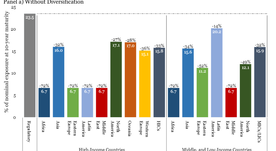
Under the heading EIOPA, Table 6 shows the 10-year exposure capital charges currently applied within Solvency II (23.5%) and those implied by our recalibration based on the credit performance of unrated infrastructure loans. These equal 15.8% for HIC exposures and 15.9% for MIC/LIC exposures. Infrastructure loans from North America or Western Europe do not exhibit a systematically better credit performance than those of exposures from other regions. So, the recalibrated capital charges are not more favourable for these typically high-income regions.
The Solvency II framework Standard Formula prescribes capital charges for credit exposures and then permits a diversification adjustment. The magnitude of this depends on the full balance sheet of the insurer in question and, hence, effective capital charges vary from insurer to insurer. In Table 6, we present calculations of Solvency II capital charges without and with diversification adjustments. The adjustments often mean that the effective capital charges are half the ‘headline’. The calculations with diversification adjustments presented in Table 6 assume that the insurer in question has the balance sheet of the stylised, example insurer described in Höring (2012). The same assumptions are employed by Kutas, Perraudin and Qiu (2016). More information about this insurer is provided in Appendix A5.
As one may observe from the results in Table 6, diversification reduces the effective capital charge for infrastructure significantly, bringing the results closer to those implied by the IAIS and Basel approaches (see below). The charge for unrated infrastructure loans under the current regulations is reduced from 23.5% to 13.0%. The charges implied by the superior ELs of infrastructure loans of 15.8% and 15.9% for HICs and LICs, respectively, are reduced by the diversification adjustment to 8.7% and 8.8%.
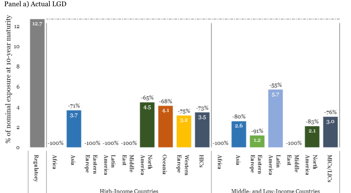
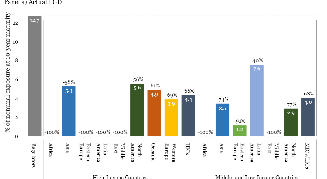
Under the heading IAIS, Table 6 displays results for the current IAIS charges for 10-year, unrated infrastructure loans (12.7%). (Recall that these are lower than those required by Solvency II in part because the latter allows a diversification adjustment after capital is first calculated.) We present recalibrated capital charges for unrated, 10-year infrastructure loans on the columns headed Method 1 and Method 2. Calculations are performed using an assumed LGD of 45% and (typically much lower) LGDs estimated using Moody’s historical data. Using Method 1, capital charges for HIC and MIC/LIC loans are, respectively, 7.1% and 8.6% when a 45% LGD is assumed. When actual historical average LGDs are employed, capital charges drop to 3.5% and 3.0%. Method 2 yields similar but slightly higher capital charges. Note that, as shown in the Appendix to this study, when risk premia are set equal to the values employed in this calibration, corporate charges are within 10% of regulatory charges for the majority of maturities and rating grades and within 20% for all such cases. Figure 1 displays the Solvency II results from Table 6 while Figures 2 and 3 (with their respective panels a) and b)) show the results for Method 1 and 2 with LGDs of 45% in the Panel a)’s and with actual LGDs in the Panel b)’s.
Panel b) With Diversification
Note: HICs stands for High-Income Countries. MICs/LICs stands for Middle- and Low-Income Countries. The two country groups HICs and MICs/LICs follow the World Bank definitions.
Panel b) Fixed LGD=45%
Note: HICs stands for High-Income Countries. MICs/LICs stands for Middle- and Low-Income Countries. The two country groups HICs and MICs/LICs follow the World Bank definitions.
Panel b) Fixed LGD=45%
Note: HICs stands for High-Income Countries. MICs/LICs stands for Middle- and Low-Income Countries. The two country groups HICs and MICs/LICs follow the World Bank definitions.
Note: HICs stands for High-Income Countries. MICs/LICs stands for Middle- and Low-Income Countries. The two country groups HICs and MICs/LICs follow the World Bank definitions.
Note: HICs stands for High-Income Countries. MICs/LICs stands for Middle- and Low-Income Countries. The two country groups HICs and MICs/LICs follow the World Bank definitions.
Note: HICs stands for High-Income Countries. MICs/LICs stands for Middle- and Low-Income Countries. The two country groups HICs and MICs/LICs follow the World Bank definitions.
| Unrated | PPP | (only) | Hist. | LGD | Method | 1 | Method | 2 | BCBS-A-IRB | (Basel | III) | ||||||
|---|---|---|---|---|---|---|---|---|---|---|---|---|---|---|---|---|---|
| Avg. | No | With | No | With | No | With | 45% | Hist. | 45% | Hist. | 40% | Hist. | |||||
| Data set | 10Y PD | LGD | Avg. EL | divers. | divers. | divers. | divers. | divers. | divers. | Curr. | LGD | LGD | LGD | LGD | Curr. | LGD | LGD |
| HICs | 4.8 | 22.1 | 1.06 | 23.5 | 13.0 | 20.0 | 11.1 | 15.8 | 8.7 | 12.7 | 7.1 | 3.5 | 8.9 | 4.4 | 3.6 | 5.8 | 3.2 |
| Africa | 1.9 | 0.0 | 0.00 | 23.5 | 13.0 | 20.0 | 11.1 | 6.7 | 3.7 | 12.7 | 4.0 | 0.0 | 6.3 | 0.0 | 2.4 | 3.8 | 0.0 |
| Asia | 4.6 | 24.3 | 1.12 | 23.5 | 12.98 | 20.0 | 11.1 | 16.0 | 8.8 | 12.7 | 6.8 | 3.7 | 9.8 | 5.3 | 3.3 | 5.3 | 3.2 |
| Eastern Europe | 12.4 | 0.0 | 0.00 | 23.5 | 12.98 | 20.0 | 11.1 | 6.7 | 3.7 | 12.7 | 12.1 | 0.0 | 12.1 | 0.0 | 5.0 | 8.0 | 0.0 |
| Latin America | 10.0 | 0.0 | 0.00 | 23.5 | 12.98 | 20.0 | 11.1 | 6.7 | 3.7 | 12.7 | 10.5 | 0.0 | 13.9 | 0.0 | 4.1 | 6.5 | 0.0 |
| Middle East | 0.3 | 0.0 | 0.00 | 23.5 | 12.98 | 20.0 | 11.1 | 6.7 | 3.7 | 12.7 | 1.1 | 0.0 | 2.3 | 0.0 | 0.9 | 1.5 | 0.0 |
| North America | 6.5 | 23.9 | 1.56 | 23.5 | 13.0 | 20.0 | 11.1 | 17.1 | 9.5 | 12.7 | 8.4 | 4.5 | 10.5 | 5.6 | 3.9 | 6.3 | 3.8 |
| Oceania | 7.3 | 20.7 | 1.51 | 23.5 | 12.98 | 20.0 | 11.1 | 17.0 | 9.4 | 12.7 | 9.0 | 4.1 | 10.6 | 4.9 | 4.1 | 6.6 | 3.4 |
| Western Europe | 4.4 | 21.2 | 0.92 | 23.5 | 12.98 | 20.0 | 11.1 | 15.1 | 8.4 | 12.7 | 6.7 | 3.2 | 8.3 | 3.9 | 3.5 | 5.6 | 3.0 |
| MICs/LICs | 7.0 | 15.8 | 1.10 | 23.5 | 13.0 | 20.0 | 11.1 | 15.9 | 8.8 | 12.7 | 8.6 | 3.0 | 11.5 | 4.0 | 3.8 | 6.1 | 2.4 |
| Africa | 1.9 | 0.0 | 0.00 | 23.5 | 13.0 | 20.0 | 11.1 | 6.7 | 3.7 | 12.7 | 4.0 | 0.0 | 6.3 | 0.0 | 2.4 | 3.8 | 0.0 |
| Asia | 7.8 | 12.7 | 0.99 | 23.5 | 12.98 | 20.0 | 11.1 | 15.6 | 8.6 | 12.7 | 9.2 | 2.6 | 12.2 | 3.5 | 3.9 | 6.2 | 2.0 |
| Eastern Europe | 13.7 | 4.2 | 0.57 | 23.5 | 12.98 | 20.0 | 11.1 | 11.2 | 6.2 | 12.7 | 12.7 | 1.2 | 12.6 | 1.2 | 5.1 | 8.2 | 0.9 |
| Latin America | 10.6 | 23.8 | 2.53 | 23.5 | 12.98 | 20 | 11.1 | 20.2 | 11.2 | 12.7 | 10.8 | 5.7 | 14.3 | 7.6 | 4.1 | 6.6 | 3.9 |
| Middle East | 0.2 | 0.0 | 0.00 | 23.5 | 12.98 | 20 | 11.1 | 6.7 | 3.7 | 12.7 | 1.0 | 0.0 | 3.0 | 0.0 | 0.8 | 1.3 | 0.0 |
| North America | 4.1 | 14.8 | 0.61 | 23.5 | 13.0 | 20.0 | 11.1 | 12.1 | 6.7 | 12.7 | 6.4 | 2.1 | 8.9 | 2.9 | 3.3 | 5.3 | 1.9 |
Note: The data inputs are based on statistics calculated by Moody’s for the sample period 1983-2018. 10Y PD is the 10-year cumulative PD from Table 5. Avg. LGD is the LGD from Table 5. Avg. EL is the product of the average annual default rate (based on the 10Y PD) and the Avg. LGD. Block headed “Unrated” under “EIOPA (SII)” is from Table 1 and Table 2. It is the capital charge for unrated debt securities and bank loans. Block headed “PPP (only)” under “EIOPA (SII)” is from Table 1 and Table 2. It is the adjusted risk factors for infrastructure investment ('Solvency II Amendment') [EEA or OECD] for unrated PPP (only). Block “Hist. LGD” under “EIOPA (SII)” contains the capital charge estimated with method described in Appendix A.1 Solvency II Calibration. Under “EIOPA (SII)”, the headers “With div.” and “No div.” indicate that the calculations are performed allowing for diversification or not. Columns headed “Curr.” contain the current regulatory capital charges. The column headed “Curr.” under “IAIS (ICS2)” is from Table 3. The column headed “Hist. LGD” uses estimated LGDs from the column “Avg. LGD” for the capital charge calculation. The column headed “45% LGD” uses a fixed LGD 45% for the capital charge calculation. This LGD is what IAIS reportedly used in calibrating the ICS2. The column headed “40% LGD” uses a fixed LGD 40% for the capital charge calculation. This is the regulatory LGD under the Foundation IRB. The column headed “Current” under “BCBS-A-IRB” uses LGDs equal to the A-IRB of 25%. This is the floor for unsecured corporate (including Specialised Lending) loans under the Basel III A-IRB.
4. Conclusion
Using credit performance statistics for infrastructure loans published by Moody’s, this paper sets out capital requirement calibrations using methods similar to those employed by regulators in determining regulatory capital charges.
The favourable credit performance of infrastructure loans relative to that of corporate debt more generally results in distinctly lower capital charges for these loans compared to the broader corporate debt asset class. This analysis provides justification for a regulatory approach in which low capital charges are applied to infrastructure debt than to the wider class of corporate debt.
Within the Solvency II framework, EIOPA has introduced lower capital charges for higher rated OECD or EEA infrastructure debt. But this favourable treatment is not extended to infrastructure debt related to projects in less developed non-EEA countries even though these too exhibit superior credit performance in the Moody’s data. The new capital framework published by IAIS (2019) in November 2019 makes no concessions, however, to infrastructure debt.
Our analysis, which consist of mimicking the calibration approaches of the regulators for the specific asset class of infrastructure loans, suggests that the capital charges for unrated infrastructure loans should be about one third lower than those required in Solvency II and between two thirds and three quarters lower than those in the IAIS rules (depending on the calibration methodology employed).
References
Basel Committee on Banking Supervision (BCBS) (2017) “Finalizing Post-Crisis Reforms,” December (Basel: Bank for International Settlements), available at https://www.bis.org/bcbs/publ/d424.htm
EIOPA (2013) “Standard Formula Design and Calibration of Certain Long-Term Investments,” Technical Report No. 13/513, available at: https://eiopa.europa.eu/Publications/Reports/EIOPA_Technical_Report_on_Standard_Formula_Design_ and_Calibration_for_certain_Long-Term_Investments__2_.pdf
EIOPA (2014) “The Underlying Assumptions in the Standard Formula for the Solvency Capital Requirement Calculation,” EIOPA-14-322, available at: https://eiopa.europa.eu/Publications/Standards/EIOPA-14- 322_Underlying_Assumptions.pdf.
EIOPA (2015a) “Infrastructure Investments by Insurers,” Discussion Paper No. CP-15-003, available at: https://eiopa.europa.eu/Publications/Consultations/EIOPA-CP-15-003_Discussion_paper_on_ Infrastructure_Investments_for_public.pdf.
EIOPA (2015b) “Call for Advice from the European Commission on the Identification and Calibration of Infrastructure Risk Categories,” Final Report on the Consultation Paper No. CP-15-004, available at: https://eiopa.europa.eu/Publications/Consultations/EIOPA-BoS-15-223%20Final%20Report%20 Advice%20infrastructure.pdf.
European Commission (2015), “Commission Delegated Regulation (EU) 2015/35 of 10 October 2014 Supplementing Directive 2009/138/EC of the European Parliament and of the Council on the Taking-up and Pursuit of the Business of Insurance and Reinsurance (Solvency II),” Official Journal of the European Union, available at http://data.europa.eu/eli/reg_del/2015/35/oj
European Commission (2016) “Commission Delegated Regulation (EU) 2016/467 of 30 September 2015 Amending Commission Delegated Regulation (EU) 2015/35 Concerning the Calculation of Regulatory Capital Requirements for Several Categories of Assets Held by Insurance and Reinsurance Undertakings,” Official Journal of the European Union, available at: http://data.europa.eu/eli/reg_del/2016/467/oj. European Commission (2017) “Commission Delegated Regulation (EU) 2017/1542 of 8 June 2017 Amending Delegated Regulation (EU) 2015/35 Concerning the Calculation of Regulatory Capital Requirements for Certain
Categories of Assets Held by Insurance and Reinsurance Undertakings (Infrastructure Corporates),” Official Journal of the European Union, available at: http://data.europa.eu/eli/reg_del/2017/1542/oj.
Höring, Dirk (2012) “Will Solvency II Market Risk Requirements Bite? The Impact of Solvency II on Insurer’s Asset Allocation,” The Geneva Papers, 38(2), pp. 250-273, July
International Association of Insurance Supervisors (2017) “Instructions for the May 2017 Quantitative Data Collection Exercise,” available at: https://www.iaisweb.org/file/67655/public-2017-field-testing-technicalspecifications.
International Association of Insurance Supervisors (2019) “Level 1 Document: ICS Version 2.0 for the monitoring period,” available at: https://kpmglexlinks.de/fileadmin/Externe_Dokumente/Versicherungen/International/IAIS/Amtsblatt/IAIS_Level_1_Doc _ICS_Version_2.0.pdf.
International Association of Insurance Supervisors (2020) “Level 2 Document: ICS Version 2.0 for the monitoring period,” available at: https://www.iaisweb.org/page/supervisory-material/insurance-capitalstandard/file/89208/level-2-document-for-ics-version-20-for-the-monitoring-period.
Jobst, Andreas A., (2018) Credit Risk Dynamics of Infrastructure Investment: Considerations for Financial Regulators, Washington DC: World Bank Group.
Karapiperis, D. (2017) “Infrastructure Investment and the Insurance Industry,” The Center for Insurance Policy and Research (CIPR) Newsletter, available at: http://www.naic.org/cipr_newsletter_archive/vol22_infrastructure.pdf
Kutas, Jozsef, William Perraudin and Yixin Qiu (2016) “Solvency II Capital Calibration for Securitisations,” available at: https://www.riskcontrollimited.com/wp-content/uploads/2016/07/Solvency-II-Calibration- Securitisations.pdf
Levy, Joaquim, (2017) “Risk and Capital Requirements for Infrastructure Investment in Emerging Market and Developing Economies,” 22nd December, available at: https://www.worldbank.org/en/news/feature/2017/12/22/risk-and-capital-requirements-for-infrastructureinvestment-in-emerging-market-and-developing-economies
Moody’s (2019) “Annual default study: Defaults will rise modestly in 2019 amid higher volatility,” 1st February, available at: https://www.moodys.com/researchdocumentcontentpage.aspx?docid=PBC_1156859
Moody’s (2020) “Examining Infrastructure as an Asset Class,” 2nd May.
Saha, D., Ho Hong, S., Modi, A. and Zemlytska, I. (2018) “Contribution of Institutional Investors Private Investment in Infrastructure 2011–H1 2017,” Private Participation in Infrastructure (PPI) Database (Infrastructure, PPPs & Guarantees Group and World Bank Group Singapore Hub for Infrastructure and Urban Development), available at: https://ppi.worldbank.org/content/dam/PPI/documents/PPI_InstitutionalInvestors_Update_2017.pdf.
Standard & Poor’s (2014) “2013 Annual Global Corporate Default Study And Rating Transitions,” 19th March.
Vasicek, Oldrich A. (2002) “The Distribution of Loan Portfolio Value,” Risk, available at: https://www.semanticscholar.org/paper/THE-DISTRIBUTION-OF-LOAN-PORTFOLIO-VALUE- Vasicek/f1f308a5c6e95fee1dd9ca3c8c51d19b5128fd59.
Appendix
A.1 Solvency II Calibration We calibrate Solvency II capital charges for infrastructure exposures by calculating the Expected Losses on an infrastructure loan in a given category and then assigning to it the capital that Solvency II requires for a general corporate loan with the same EL.
corp denote the expected loss (per year of duration) for corporate issuer with credit To state this formally, let ELt,i C may be expressed formally as follows. quality step i for horizon [0, t). ELt,i
C (A1) ELCt,i = Pt,iC × LGDi
C is the cumulative PD for a C is the loss given default for credit quality step i, i ∈[0,1,2,3,4,5]. Pt,i Here, LGDi corporate issuer with credit quality step i over the horizon [0, t).
C denote the regulated risk factor for corporate issuers with maturity t and credit quality step i. This can Let bt,i be found in Table 1.
I denote the expected loss for unrated infrastructure debt for horizon [0, t) Let ELt
I × LGDI (A2) ELIt = Pt
I is the cumulative PD for an unrated Here, LGDI is the loss given default for the infrastructure debt. Pt infrastructure loan over the horizon [0, t).
I, t≤5 is obtained by Let btI denote the regulated risk factor for corporate issuers with maturity t and rating i. bt linear interpolation as shown in equation (A3).
C bt,0C , if ELIt ≤ELt,0 C bt,jC −bt,i , ifELCt,i < ELIt ≤ELCt,j I = C + C ) , t≤5 (A3) bt bt,j C × (ELIt −ELt,i ELCt,j−ELt,i C bt,5C , ELIt ≥ELt,5 {
C btI, 5 < t≤10 is derived similarly as in equation (A3) except replace ELIt and ELCt,i with ∆ELIt and ∆ELt,i respectively. Here, C (A4) ∆ELIt = ELtI −EL[5]I , ∆ELCt,i = ELtC −EL[5]
I, 5 < t≤10 is then calculated as shown below bt
C bt,0C , if ∆ELIt ≤∆ELt,0 C bt,jC −bt,i , if ∆ELCt,i < ∆ELIt ≤∆ELCt,j I = C + C ) , 5 < t≤10 (A5) bt bt,j C × (∆ELIt −∆ELt,i ∆ELCt,j−∆ELt,i C bt,5C , ∆ELIt ≥∆ELt,5 {
The 10-year capital charges presented in column “RCL” under section “EIOPA (SII)” in Table 5 is then calculated as: I × (10 −5) (A6) capital(10) = b[5]I × 5 + b[10]
A.2 ICS Calibration Using Method 1 This method is based on Vasicek (2002). Vasicek shows how to calculate the Expected Loss (EL) at date 1 on a t>1 maturity loan (i) conditional on a common factor and (ii) with risk adjusted distribution. Conditioning on a 99.5% stress event implies that the EL equals the Marginal Value at Risk (MVaR) for the exposure in question and, hence, equals capital. The use of a risk-adjusted distribution implies that the capital allows for the repricing risk at the 1-year horizon.
Given a set of cumulative PDs for horizons [0,1), [0,2), … [0, t) measured at date 0.
P0,1, P0,2, … P0,t
The capital is calculated as
T ρ capital= exp(−r× (T−1)) × LGD× Φ (b(T) × √ T−ρ −Φ−1(α) × √T−ρ) (A7)
Here, r is the bond interest rate, assumed to be 5%. Φ is the cumulative distribution function for standard Gaussian distribution. Φ−1 is the inverse cumulative distribution function for standard Gaussian distribution b(t) is calculated as T−1 b(t) = Φ−1(P0,t ) + λ× ρM × √T (A8)
Here, λ= 1.1 and ρM = 0.2. The parameter values are calibrated so that the calibrated capitals are all within 20% differences compared to the regulatory capital shown in Table 4 using Method 2 (described in Section A.3) and S&P 2013 data. In the above equations, the parameter ρ is calculated as a function of the 1-year default probability: 1−exp (−50×PD0,1) 1−exp (−50×PD0,1) ρ= 0.12 × + 0.24 × (1 − ) (A9) 1−exp (−50) 1−exp (−50)
A.3 ICS Calibration Using Method 2 This method is calculated based on the formula in Jobst (2018).
With the same notation as in the Subsection A.2, the 1-year forward PD P1,t is defined as
P0,t − P0,1 P1,t ≡ 1− P0,1 (A10)
The risk-adjusted forward PD Q1,t is then calculated as
Q1,t = Φ( Φ−1(P1,t) + λ× ρM × √t−1 ) (A11)
The risk-adjusted PD Q0,t is then calculated as
Q0,t = Φ( Φ−1(P0,t) + λ× ρM × √t−1 ) (A12)
∗ is the expectation shown below. The stressed risk-adjusted forward PD Q1,t
Φ−1(P0,t)√t−(√ρΦ−1(α)−√1−ρZ) ∗ = Ε [Φ ( Q1,t + λρM√t−1)] (A13) √t−1
Here, Z follows standard Gaussian distribution.
The expectation in equation (A13) is calculated through the numerical integral
Φ−1(P0,t)√t−(√ρΦ−1(α)−√1−ρk∆x) 1 2(k∆x)2 N ∗ = ∑ Φ ( ) ∆x (A14) Q1,t k=−N + λρM√t−1) × √t−1 √2π × exp (− 2
Here, ∆x=0.0001 and N = 1000,000. In the above equations, λ= 1.1 and ρM = 0.2. The parameter values are calibrated so that the calibrated capital charges for rated corporate exposures are all within 20% of the regulatory capital charges for corporate exposures shown in Table 4 using this method and S&P 2013 data. Details of the calibration are provided below.
The capital is calculated as:
Φ−1(P0,1)−√ρ×Φ−1(α) capital= LGD× Φ ( ) + LGD× exp (−r) × (Q1,t∗ −Q1,t) (A15) √1−ρ
Table A.1 presents the corporate cumulative default rates from S&P (2013).
Table A.1: Global Corporate Average Cumulative Default Rates (1981-2013) (%)
Maturity (yrs)
Rating 1 2 3 4 5 6 7 8 9 10 11 12 13 14 15
AAA 0.0 0.0 0.1 0.2 0.4 0.5 0.5 0.6 0.7 0.7 0.8 0.8 0.8 0.9 1.0
AA 0.0 0.1 0.1 0.2 0.4 0.5 0.6 0.7 0.8 0.8 0.9 1.0 1.1 1.2 1.2
A 0.1 0.2 0.3 0.4 0.6 0.8 1.0 1.2 1.4 1.6 1.8 2.0 2.1 2.3 2.5
BBB 0.2 0.6 1.0 1.5 2.1 2.6 3.0 3.5 3.9 4.3 4.8 5.2 5.5 5.9 6.3
BB 0.8 2.5 4.4 6.3 8.0 9.6 11.0 12.3 13.4 14.4 15.2 15.9 16.5 17.1 17.6
B 4.1 9.3 13.6 17.0 19.6 21.6 23.3 24.7 25.8 27.0 28.0 28.8 29.5 30.2 30.8
CCC/C 26.9 36.1 41.2 44.3 46.8 47.8 48.9 49.7 50.6 51.4 52.0 52.8 53.7 54.4 54.4
Inv Grade 0.1 0.3 0.5 0.8 1.1 1.4 1.6 1.9 2.1 2.4 2.6 2.8 3.0 3.2 3.4
Spec Grade 4.0 7.9 11.2 13.9 16.0 17.8 19.3 20.6 21.7 22.8 23.7 24.4 25.1 25.7 26.3
All rated 1.5 3.0 4.3 5.4 6.4 7.1 7.8 8.4 8.9 9.4 9.9 10.2 10.5 10.8 11.1 Note: The data is the Table 24 from Standard & Poor’s (2014).
To calibrate the risk parameter λ and ρM for risk adjusted PD calculation in Method 1 and Method 2 under ICS calibration, we used the corporate PD in Table A.1 from S&P (2013) and LGD=0.45 as the input data and ICS Method 2. By fixing ρM = 0.2, we tried different value of λ so that the calibrated capitals are within 20% difference to the regulated capital in as many cases as possible.
Tables A.2 to A.4 show the calibrated results for λ from 1 to 1.2. It indicates that when λ= 1.1, it has the most cases within 20% differences to the regulatory capital and within 10% differences to the regulatory capital. Therefore, λ= 1.1 and ρM = 0.2 as the final calibrated parameters.
Table A.2: Calibrated Capital (%) with λ= 1 and LGD=0.45 ICS S&P Maturity (yrs)
RC Rating 1 2 3 4 5 6 7 8 9 10 11 12 13 14 15
1 or 2 AAA/AA 0.2 0.6 0.8 1.0 1.3 1.4 1.6 1.7 1.8 1.9 2.0 2.0 2.1 2.2 2.2 10% difference to
3 A 0.6 1.4 1.6 1.9 2.1 2.3 2.6 2.7 2.9 3.0 3.1 3.2 3.3 3.4 3.5 regulatory capital
4 BBB 1.4 3.5 3.9 4.4 4.7 5.0 5.1 5.3 5.4 5.5 5.5 5.6 5.6 5.6 5.6
5 BB 3.6 8.6 9.4 9.8 10.0 10.0 9.9 9.8 9.6 9.5 9.3 9.2 9.0 8.8 8.7 10%-20% difference
6 B 8.9 18.2 18.1 17.6 17.1 16.6 16.2 15.8 15.5 15.1 14.8 14.6 14.3 14.1 13.9 to regulatory capital
7 CCC/C 27.7 48.9 45.7 43.6 42.0 41.1 40.2 39.5 38.8 38.2 37.6 37.1 36.5 36.0 35.8 Note: ICS RC stands for the ICS Rating Category.
Table A.3: Calibrated Capital (%) with λ= 1.1 and LGD=0.45 ICS S&P Maturity (yrs)
RC Rating 1 2 3 4 5 6 7 8 9 10 11 12 13 14 15
1 or 2 AAA/AA 0.2 0.6 0.8 1.1 1.3 1.5 1.7 1.8 1.9 2.0 2.1 2.2 2.3 2.3 2.4 10% difference to
3 A 0.6 1.4 1.7 2.0 2.2 2.4 2.7 2.9 3.0 3.2 3.3 3.4 3.5 3.6 3.7 regulatory capital
4 BBB 1.4 3.6 4.0 4.5 4.9 5.1 5.3 5.4 5.6 5.7 5.7 5.8 5.8 5.8 5.8
5 BB 3.6 8.7 9.6 10.0 10.1 10.1 10.0 9.9 9.7 9.5 9.4 9.2 9.0 8.8 8.7 10%-20% difference
6 B 8.9 18.3 18.1 17.7 17.1 16.6 16.2 15.8 15.4 15.1 14.7 14.5 14.2 13.9 13.7 to regulatory capital
7 CCC/C 27.7 48.9 45.6 43.5 41.8 40.9 39.9 39.2 38.4 37.8 37.3 36.7 36.1 35.6 35.3 Note: ICS RC stands for the ICS Rating Category.
Table A.4: Calibrated Capital (%) with λ= 1.2 and LGD=0.45 ICS S&P Maturity (yrs)
RC Rating 1 2 3 4 5 6 7 8 9 10 11 12 13 14 15
1 or 2 AAA/AA 0.2 0.6 0.8 1.1 1.4 1.6 1.8 1.9 2.0 2.2 2.3 2.4 2.5 2.5 2.6 10% difference to
3 A 0.6 1.5 1.7 2.0 2.3 2.6 2.8 3.0 3.2 3.4 3.5 3.6 3.7 3.8 3.9 regulatory capital
4 BBB 1.4 3.6 4.1 4.6 5.0 5.3 5.5 5.6 5.8 5.8 5.9 5.9 6.0 5.9 5.9
5 BB 3.6 8.8 9.7 10.1 10.2 10.2 10.1 10.0 9.8 9.6 9.4 9.2 9.0 8.8 8.6 10%-20% difference
6 B 8.9 18.4 18.2 17.7 17.2 16.6 16.2 15.7 15.3 15.0 14.6 14.3 14.0 13.8 13.5 to regulatory capital
7 CCC/C 27.7 48.9 45.5 43.4 41.6 40.6 39.6 38.9 38.1 37.4 36.8 36.3 35.6 35.1 34.9 Note: ICS RC stands for the ICS Rating Category.
A.5 BCBS (Basel III) With the same notation as in Subsection A.2, the capital charge in Basel III formula (see BCBS (2017)) is calculated as below:
P0,t Φ−1( t )−√ρ×Φ−1(α) P0,t 1+(t−2.5)b (A16) capital= (LGD× Φ ( ) −LGD× t ) × 1−1.5b √1−ρ
Here, b is calculated as
P0,t b= (0.11852 −0.05478 × ln ( (A17) t ))
A.5 Capital Diversification Under the Solvency II rules, capital is calculated for exposures on a standalone basis and then an adjustment is made for diversification. This means that the ‘headline’ capital charge is not the one that actually applies. The latter depends on the insurer’s portfolio.
In order to calculate the capital diversification effect, we consider a representative European life insurer as described in Höring (2012) with EUR 4 billion as total assets and EUR 3 billion as its market risk portfolio. Table A.5 shows the assumed breakdown of the market risk portfolio.
To calculate the capital requirement for the spread risk sub-module, the modified duration of each exposure is required. For the sake of simplicity, we suppose that exposures in each asset class have a single representative duration as shown in Table A.6.
The durations of assets and liabilities for Höring’s representative insurer are assumed to be 6.8 and 8.9 years, respectively. To calculate capital for the interest rate risk sub-module, an average downward interest rate shock is calculated using the March 2016 risk free curves provided by EIOPA. This is multiplied by the difference of 2.1 between the liability and asset durations and the result is multiplied by the asset total of EUR 4 billion.
Table A.5: The market risk portfolio of a representative European life insurer Rating Sub-module Subtype AAA AA A BBB BB ≤B Unrated Total Type 1 - - - - - - - 4.5 Equity Type 2 - - - - - - - 2.5 Property - - - - - - - 11.0 Bonds 5.2 4.4 11.8 5.9 0.6 0.1 1.5 29.5 Covered bonds 11.5 0.5 0.3 0.1 - - 0.1 12.5 Spread Sovereign debt (EEA) 18.8 6.6 5.8 0.2 0.6 - - 32.0 Sovereign debt (Non-EEA) 5.2 1.4 0.2 0.8 - 0.2 0.2 8.0 Note: The market risk portfolio of a representative European-based life insurer is shown broken down by Solvency II sub-module, and further broken down by the subtypes considered in each sub-module and the credit rating of exposures considered in the spread risk sub-module. The entries are given as a percentage of the total EUR 3 billion value of the market risk portfolio.
Table A.6: Modified duration by asset class Asset class Modified duration (years) Bonds 5.4 Covered bonds 6.2 Sovereign debt 6.9 Note: These values show the average modified duration of exposures of different asset classes treated under the market risk module for a representative Europeanbased life insurer. The values are provided in Höring (2012).
Risk Control 13-14 Dean Street London W1D 3RS +44(0)2033070730 www.riskcontrollimited.com
Notes
[1] This study was commissioned from Risk Control by Global Infrastructure Hub.
[2] A note on this reconciliation is available from the authors upon request.