

This paper provides a comment on the Regulatory Technical Standard (RTS) recently issued by the European Banking Authority’s (EBA) on the use of the Purchased Receivables Approach (PuRA) by European banks. The RTS is designed to clarify an important component of the Basel 3 rules for securitisation capital as applied to banks in Europe. The PuRA would be used by banks to calculate inputs to the SEC-IRBA, the most advanced of the hierarchy of approaches that banks are permitted to employ when calculating regulatory capital for securitisation exposures in the banking book. To illustrate the implementation of the PuRA, we estimate a set of models based on European Data Warehouse (ED) data for residential mortgages. We estimate models for 8 European countries using loan level data for the pools of 504 Residential Mortgage Backed Security deals. We are able to formulate models at country, originator and deal levels. We examine how data from these different models may be combined to estimate PDs for a single notional deal. We discuss how adjustments may be made for originator underwriting standards and for different Margins of Conservatism. The exercises we perform help us to identify ways in which the EBA’s RTS could be helpfully extended or made more precise. We conclude that there are three areas in which the RTS could be clarified. First, the RTS state that the data hierarchy for banks implementing the PuRA is the inverse of what would normally hold for an IRB model implementation in that external data on exposures resembling those of the securitisation pool in question should be preferred to the bank’s internal data on loans that it has originated itself. This implies that PuRA modelling should be considered as the development of a methodology that can be applied to multiple datasets in a dynamic way as securitisation deals present themselves. It would be helpful for the EBA to acknowledge this as it represents a significant departure from the usual IRB modelling practice and has multiple important implications. Second, the EBA has provided little guidance in the crucial area of what data is acceptable. A key question is whether aggregate performance data of the sort contained in securitisation market investor reports and used by ratings agencies in risk analysis of securitisations may serve as the basis for analysis or whether loan level data is essential to obtain supervisory approval. This study employs loan level data but we are aware that ratings agencies often analyse securitisations on the basis of cumulative default curves broken down by vintage. Third, the EBA’s 2017 guidelines on IRB modelling require banks implementing IRB models to develop Margins of Conservatism and to allow for the impact of underwriting standards. While significant in other IRB exercises, these two requirements are central to PuRA modelling involving as it does multiple data sources used in a varied and dynamic way. Making all aspects of these activities fully statistical and data driven (without judgmental input) appears scarcely feasible. Acknowledging this even while stipulating that any judgments be prudent and evidence-based would be helpful.
1. Introduction
The Basel 3 regulatory capital rules for banking book securitisation exposures permit banks to use a hierarchy of approaches. These include the Securitisation Internal Ratings-based Approach (SEC-IRBA), the Securitisation Standardised Approach (SEC-SA) and the Securitisation External Ratings-based Approach (SEC- ERBA).[1]
As implemented within the Europe Union, the Basel rules require banks to use, if possible, the SEC-IRBA, followed by the SEC-SA or the SEC-ERBA. Duponcheele, Linden and Perraudin (2016) show that, for a large fraction of the European securitisation market, the SEC-IRBA yields lower capital than the alternative approaches. It has, nevertheless, been doubtful whether European banks would be able to employ the SEC- IRBA for securitisation deals other than those for which they themselves are the originators.[2]
The reason is that the SEC-IRBA requires as input the capital that the pool assets would attract under Basel if they were held on balance sheet (in the Basel terminology: ‘KIRB’). Estimates of KIRB are subject to stringent data standards. National regulators, even within Europe, vary significantly in how strictly they enforce these standards. At various stages through the development of the Basel 3 securitisation capital rules, regulators have suggested that KIRB for securitisation capital purposes might be estimated using proxy data. But the precise nature of any possible relaxation in data standards has never been clarified and some regulators point to the fact that proxy data is already allowed for under the usual IRB approaches.
The European implementation of Basel 3 (see the Capital Requirements Regulation (CRR)) envisages that banks wishing to calculate KIRB for securitisation capital purposes may employ existing CRR provisions for Purchased Receivables. The Purchased Receivables Approach (PuRA) allowed for under the CRR has, in fact, been employed by few European banks. Most have preferred to purchase client-originated receivables through conduits and then to calculate capital using the Internal Assessment Approach (IAA).
Partly because of a lack of experience in the use of PuRA and partly because of doubts as to how regulators will enforce data standards, most banks have viewed the SEC-IRBA as inaccessible. Since the SEC-IRBA implies more risk-based and possibly somewhat lower capital than other approaches, inability to apply this approach would reduce the scope for European banks to participate in the securitisation market.
This would significantly favour banks from other jurisdictions. Among these, US banks already have ready access to the Supervisory Formula Approach (SFA). US bank regulators have for some time permitted their banks to calculate KIRB as inputs to the SFA for securitisation pools that these banks have not originated themselves. The same key input of KIRB is required by the SFA and SEC-IRBA so there is little doubt that US banks will have straightforward access to the latter under the new rules.
To clarify what European banks will have to do to access the SEC-IRBA, the European Banking Authority (EBA) has issued draft Regulatory Technical Standards (RTS) on the use of the PuRA for securitisation capital (see EBA (2018)). The RTS help to clarify how the operational standards of PuRA would apply to securitisations. The Basel and CRR rules for Purchased Receivables contain a series of requirements having to do with control and monitoring of the assets.
Clearly, for a bank buying receivables from a non-financial firm, an issue is who controls the receivables in the event of credit event affecting the seller. Also, mechanisms may not be very well established for monitoring non-financial receivables. Hence, robust arrangements must be described in regulations pertaining to a bank purchasing such receivables. The EBA’s RTS are helpful in explaining how these aspects of the purchased receivables rules should be interpreted when this section of the capital rules is applied to securitisation exposures.
The EBA’s RTS also contain a set of statements regarding how a bank employing the PuRA in the context of the SEC-IRBA should approach the modelling tasks involved. Key statements include: (a) banks must develop dedicated IRB models rather than relying on existing models calibrated off loans the bank has originated itself,
(b) banks must allow for differences in the underwriting standards of the originator of the assets in question, (c) the hierarchy of data to be employed in the PuRA will often be the inverse of the usual one in IRB modelling exercises in that internal data will generally be least applicable while external data (if pertaining to exposures closely resembling those in the securitisation pool) will be most applicable.
This paper comments on the EBA RTS by analysing the logic of the above statements and examining what they imply for a bank implementing a PuRA framework. To illustrate the points we make, we develop an example suite of PuRA models for residential mortgages from 8 European countries. Implementing these models, we are able to illustrate the specific challenges that a bank will face in implementing the SEC-IRBA using the PuRA.
While we can illustrate the issues involved, it remains unclear how supervisors will react different solutions that banks might propose. We, therefore, believe that it would be helpful if the EBA laid more of a groundwork for the supervisory treatment of PuRA models by providing greater precision in quantitative modelling aspects.
This paper is organised as follows. Section 2 describes the SEC-IRBA and how regulators have suggested banks might implement it. This section covers the CRR text itself and additional information contained in the EBA’s June 2018 draft RTS. Section 3 sets out an example PuRA implementation for European residential mortgage loans. Sections 4, 5 and 6 discuss the implications of an inverted data hierarchy, underwriting standards and Margins of Conservatism, respectively. Section 7 discusses topics on which greater clarity by the EBA would be helpful and Section 8 concludes. An appendix provides some information on data quality, illustrating some of the challenges in dealing with loan level data.
2. The SEC-IRBA and its Implementation
2.1 Overview of SEC-IRBA
The CRR Amendment Regulation (2017) applies a hierarchy of approaches for determining the capital requirements for securitisation exposures as introduced in the BCBS 424 publication. First in the hierarchy is the SEC-IRBA. If the SEC-IRBA cannot be applied, then the SEC-SA may be used. Where neither the SEC-IRBA nor the SEC-SA can be applied, the SEC-ERBA may be employed. Finally, if none of the above approaches can be applied then a risk weight of 1,250% is used.
A bank can employ the SEC-IRBA only if it has enough information to calculate KIRB, the regulatory capital charge had the underlying exposure not been securitized, for either all the exposures in an IRB pool or for at least 95% of the exposures in a mixed pool. An IRB pool refers to a pool of underlying exposures of a type in relation to which the institution has permission to use the IRB Approach and is able to calculate risk- weighted exposure amounts for all of these exposures. The pool of underlying exposures is referred to as a mixed pool if the institution is able to calculate the risk- weighted exposure for some, but not all, of the exposures.
The main input for calculating the risk weights, denoted RW, for securitisation exposure is KIRB. Other inputs include the attachment and detachment points, A and D respectively, tranche maturity, MT, and a supervisory parameter, p. The KIRB is determined by multiplying the risk-weighted exposure amounts by 8 % divided by the exposure value of the underlying exposures.
The risk-weights are assigned based on the KIRB, A and D as follows: RW= 1250%, D≤KIRB RW= 12.5 × KSSFA(KIRB), A≥KIRB KIRB−A D−KIRB RW= [( (1) D−A ) × 12.5] + [( D−A ) × 12.5 × KSSFA(KIRB)] , A< KIRB < D.
Here, KSSFA(KIRB) is the capital requirement per unit of securitisation exposure and calculated as, ea∙u−ea∙l KSSFA(KIRB) = a(u−l)
a= −( p×KIRB) u= D−KIRB l= max(A−KIRB, 0) p= max [0.3, A+ B× ( (2) N) + C× KIRB + D× LGD+ E× MT] Here, N is the effective number of exposures in the pool of underlying exposures, LGD is the exposure-weighted average loss-given-default of the pool of underlying exposures, MTis the maturity of the tranche. The parameters A, B, C, D, and E are determined according the following table.
Note that the CRR Amendment Regulation (2017) allows for tranche maturity to be calculated either as the weighted average maturity of the contractual payments due or based on the final legal maturity of the tranche.
Using the contractual payments including the principle, interest and fees payable by the borrower, the tranche maturity can be calculated as, ∑t∙CFt t (3) MT = ∑CFt t Here, CFt is the total payment due during period t.
The other alternative is using the maximum legal maturity, ML where the tranche maturity can be determined as: MT = 1 + (ML −1) × 0.8. (4)
A floor of 1 year and a cap of 5 years is finally applied to the calculated tranche maturities.
| A | B | C | D | E | |
|---|---|---|---|---|---|
| Senior, granular (N≥25) | 0 | 3.56 | -1.85 | 0.55 | 0.07 |
| Senior, non-granular (N<25) | 0.11 | 2.61 | -2.91 | 0.68 | 0.07 |
| Non-senior, granular (N≥25) | 0.16 | 2.87 | -1.03 | 0.21 | 0.07 |
| Non-senior, non-granular (N<25) | 0.22 | 2.35 | -2.46 | 0.48 | 0.07 |
| Senior | 0 | 0 | -7 .48 | 0.7 1 | 0.24 |
| Non-Senior | 0 | 0 | -5.7 8 | 0.55 | 0.27 |
Note: This table shows the values to be used for calculating the supervisory parameter, p.
2.2 PuRA and the EBA’s Draft RTS
The PuRA refers to the IRB framework of the CRR on the treatment of purchased receivables. The CRR permits banks that purchase corporate receivables from other financial institutions to use the IRB retail approaches for calculating regulatory capital. The CRR Amendment Regulation (2017) explicitly states that the banks may apply the purchased receivables framework in calculation of the KIRB for the SEC-IRBA. Table 2 presents the relevant text from the CRR Amendment that states the possibility for the banks to use the PuRA for securitisation exposures.
255(1), underlying exposures of the securitisation in accordance with … the calculation of capital 255(4) requirements for purchased receivables. For these purposes, retail exposures shall be treated as purchased retail receivables and non-retail exposures as purchased corporate receivables."
Note: This table presents the text for application of the PuRA framework for securitisation exposures. The source is the Regulation (EU) 2017/2401 of the European Parliament and of the council of 12 December 2017 amending Regulation (EU) No 575/2013 on prudential requirements for credit institutions and investment firms.
The EBA’s draft RTS sets out the requirements that an institution has to meet to use the PuRA for securitisation exposures. In what follows, we shall consider the implications of the RTS, focussing particularly on implications for the quantitative modelling that banks will have to employ to implement the SEC-IRBA.
On which banks can use the PuRA approach, Article 2 states two sets of requirements that must be met. First, the bank may not be a servicer of the pool assets. Second, the bank must meet operational requirements for the purchased receivables approach.[3] By Article 3 of the RTS, banks that use PuRA must already have permission to employ the IRB approach “for at least one rating system within the exposure class to which the securitised exposures are assigned.” Furthermore “the experience required for that permission shall be considered sufficient prior experience for the purposes of this Regulation.”
Key points relating to quantitative modelling include Article 5 on “General conditions for risk differentiation” and Article 9 on “Requirements on data”.
Article 5 states that: “When assigning exposures to grades or pools, institutions shall consider the originator’s underwriting standards and the servicer’s recovery practices and servicing standards as risk drivers, unless they use different calibration segments for different originators and different servicers in quantifying the risk parameters associated with those grades or pools.”
Such a requirement that the under-writing standards of the originator be explicitly considered is challenging. Purchasers of bank loan pools are well aware that the credit performance of loan portfolios depends as much on underwriting standards as on the stage of the business cycle. But, observing differences in such standards or being able to measure them statistically is not straightforward. An investor in bank loan portfolios might engage in due diligence, inspecting loan files and comparing what is found to documented policies of the originator. Such an investor effectively bears the whole risk of a pool. For an investor in a mezzanine or senior exposure, it may not be appropriate to perform such intensive due diligence so a more statistically based evaluation of underwriting standards is more appropriate but difficult to implement.
Article 9 (“Requirements on data”) states that: “1. Where the securitised exposures and the obligors of those exposures were, before the transfer of such exposures to the SSPE, not obligors or exposures of the institution calculating KIRB, instead of the requirement of representativeness of the data used for model development in accordance with Article 174(c) of Regulation (EU) No 575/2013, the representativeness of the data shall be assessed in relation to the securitised exposures.” Also, it states that “2. Instead of the requirement in the first sentence of Article 180(2) (c) of Regulation (EU) No 575/2013, institutions shall regard data related to the securitised exposures as the primary source of information for estimating loss characteristics.”
This article effectively reverses the usual data hierarchy encountered in IRB modelling. In developing conventional IRB models for a bank’s on balance sheet loan book, internal data are preferred and external data only become applicable if internal data are scarce or unavailable. In the context of PuRA, the EBA is emphasises the need to rely, if these are available, on external data that is closely comparable to the pool under consideration.
Note that the PuRA (as set out in the CRR Amendment (2017) and clarified in the RTS) allows banks to use certain IRB modelling approaches that are not generally available in a standard IRB context. Specifically, a bank may employ a Retail Standard approach for corporate purchased receivables that satisfy certain requirements[4]. Under the Retail Standard (also called the Top Down approach in Basel documents), banks may calculate PDs for homogeneous loan pools rather than by implementing a statistical default prediction model on a loan by loan basis. Also, a bank may estimate a pool PD or LGD by using one of these two quantities in conjunction with an estimate of a pool level losses.
These are important relaxations in data and modelling requirements for receivables from non-financial originators for which data may not be recorded in ways that are standard in the banking industry. For example, loss data may be stored rather than default events and recoveries. It may also be somewhat more straightforward to calculate pool level PDs and LGDs rather than employing regression-style models to predict defaults and mean LGDs at a loan level. However, if conventional loan level securitisation pool data is available then the challenge of implementing loan-level regressions model is not major and so these concessions are not very significant, in our view.

2.3 CRR data requirements for IRB modelling
If one leaves aside operational requirements and the relaxations just described of some IRB requirements, PuRA comes to resemble standard IRB modelling with the data and procedural requirements specified in the CRR and expanded in the EBA’s 2007 guidelines on IRB PD and LGD analysis (see EBA (2017)).
Default definition 178(1)(b) “the obligor is past due more than 90 days on any material credit obligation to the institution, the parent undertaking or any of its subsidiaries. Competent authorities may replace the 90 days with 180 days for exposures secured by residential property or SME commercial immovable property in the retail exposure class, as well as exposures to public sector entities…” 178(4) “Institutions that use external data that is not itself consistent with the definition of default laid down in paragraph 1, shall make appropriate adjustments to achieve broad equivalence with the definition of default.” Length of data 180(1)(h) “the length of the underlying historical observation period used shall be at least five years for at least one source…. institutions which have not received the permission … to use own estimates of LGDs or conversion factors may use, when they implement the IRB Approach, relevant data covering a period of two years…” 180(2)(e) “irrespective of whether an institution is using external, internal or pooled data sources or a combination of the three, for their estimation of loss characteristics, the length of the underlying historical observation period used shall be at least five years for at least one source…. Subject to the permission of the competent authorities, institutions may use, when they implement the IRB Approach, relevant data covering a period of two years. The period to be covered shall increase by one year each year until relevant data cover a period of five years” Representativeness 174(c) “the data used to build the model shall be representative of the population of the institution's actual obligors or exposures” 179(2)(b) “the pool is representative of the portfolio for which the pooled data is used” Comprehensiveness 179(1)(a) “an institution's own estimates of the risk parameters PD, LGD, conversion factor and EL shall incorporate all relevant data, information and methods…” 180 “For purchased retail receivables, institutions may use external and internal reference data. Institutions shall use all relevant data sources as points of comparison.”
Benchmarking 185(c) “institutions shall also use other quantitative validation tools and comparisons with relevant external data sources…”
Maintenance 176(2) “For exposures to corporates, institutions and central governments and central banks, and for equity exposures …. institutions shall collect and store: (a) complete rating histories on obligors and recognised guarantors … (g) data on the PDs and realised default rates associated with rating grades and ratings migration.”
Tables 3 and 4 set out important passages from the CRR text on IRB models for PDs and LGDs. Key requirements for both PDs and LGDs fall into the following six categories: (i) default definition, (ii) length of data sample, (iii) representativeness, (iv) comprehensiveness, (v) benchmarking and (vi) maintenance. These basic requirements are then expanded in the EBA 2017 Guidelines which set out in detail supervisors’ expectations as to how European banks will implement IRB models.
Default definition 178(1)(b) “the obligor is past due more than 90 days on any material credit obligation to the institution, the parent undertaking or any of its subsidiaries. Competent authorities may replace the 90 days with 180 days for exposures secured by residential property or SME commercial immovable property in the retail exposure class, as well as exposures to public sector entities…” 178(4) “Institutions that use external data that is not itself consistent with the definition of default … shall make appropriate adjustments to achieve broad equivalence with the definition of default.” Length of data 181(1)(j) “for exposures to corporates, institutions and central governments and central banks, estimates of LGD shall be based on data over a minimum of five years, increasing by one year each year after implementation until a minimum of seven years is reached, for at least one data source...” 181 “For retail exposures, estimates of LGD shall be based on data over a minimum of five years…. Subject to the permission of the competent authorities, institutions may use, when they implement the IRB Approach, relevant data covering a period of two years. The period to be covered shall increase by one year each year until relevant data cover a period of five years.”
Representativeness 174(c) “the data used to build the model shall be representative of the population of the institution's actual obligors or exposures”
179(2)(b) “the pool is representative of the portfolio for which the pooled data is used” Comprehensiveness 179(1)(a) “an institution's own estimates of the risk parameters PD, LGD, conversion factor and EL shall incorporate all relevant data, information and methods….”
181(1)(a) “institutions shall estimate LGDs by facility grade or pool on the basis of the average realised LGDs by facility grade or pool using all observed defaults within the data sources (default weighted average)”
181(2)(c) “For purchased retail receivables use external and internal reference data to estimate LGDs…” Benchmarking 185(c) “institutions shall also use other quantitative validation tools and comparisons with relevant external data sources…”
Maintenance 176(4)(g) “Institutions using own estimates of LGDs and conversion factors shall collect and store…data on the components of loss for each defaulted exposure.”
176(5)(c) “For retail exposures, institutions shall collect and store…. the identity of obligors and exposures that defaulted”
The EBA 2017 guidelines helpfully describe how supervisors conceive of an IRB model at a high level, describing its central component as a “rating system”. This is depicted in Figure 1. The high-level modules are PD and LGD models and other risk assessment methods (consisting typically of tools for estimating Exposure at Default (EAD) and modelling risk in NPL portfolios). The PD model is then broken down into a set of submodules that serve to rank individual exposures by credit quality. Many banks employ a given sample to place exposures in a rank order and then, in a second step, calibrate default probabilities for subsets of the rank-ordered loans. This approach permits some flexibility in the sample used for ranking while ensuring that the final calibrated PDs accurately represent the required loan default probabilities. Common approaches to LGD modelling typically follow a simpler one-step approach.
Note that in the above described rating system, different ranking and calibration segments might be used for subsets of loans that the modeller believes are likely to exhibit different credit behaviour. Under the Retail Standard, calculations might be performed by taking averages for homogeneous pools. Otherwise, banks employ regressions models such as logit models for each ranking method and non-linear regression models for LGD analysis.
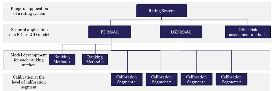
Note: This figure presents a schematic depiction of a possible rating system. The source is the EBA 2017 Guidelines on PD estimation, LGD estimation and the treatment of defaulted exposures.
3. Example Implementation of PuRA
3.1 Methodology
In this section, we describe how we implemented PD and LGD calculations for mortgage loans using data from the European Data Warehouse. The exercise is instructive as it shows what a bank may have to do to satisfy the PuRA rules and what additional guidance from the EBA may be helpful to industry modellers.
The methodology we follow in implementing the model is similar to many IRB models that we have observed in use in major banks. We have implemented this methodology in software that can be conveniently applied to large datasets of loan credit histories. It is interesting to review the steps involved in a typical IRB modelling exercise in order to understand the challenges involved in doing so for large numbers of different datasets in a dynamic way (as is required by PuRA). The steps in our methodology are as follows.
1. Data preparation
a. Retrieve and clean data b. Select samples - In this step, one can define different filtering criteria to remove irrelevant raw data and to generate a suitable dataset for modelling.
2. Formulate a regression model - Currently, our approach allows for 2 regression models, logistic and probit model. We are in the process of implementing a neural nets approach. a. Logistic regression b. By denoting default probability as PD and potential right-hand side explanatory variables as [x[1], … , xn], logistical model is expressed by equation (5). PD= 1+eβ0−∑xiβi (5)
3. Univariate Analysis
a. Coverage and distribution in relation to default events - In this step, one analyses, for each selected variable, coverage and distribution. Coverage provides information about the quality of individual variable.
b. Accuracy analysis - Logit models are estimated for each variable and their accuracy in forecasting defaults assessed. Here PD represents default probability. PD= (6) 1+eβ0−β1X
4. Data transformation
Variables are transformed in multiple ways. a. Winsorisation - This sets extreme values to given lower or upper limits. b. Accumulation points - Denote V as the dummy variables can be created for particular values of explanatory variables c. Power transformations - For some variables, power transformation result can be used to increase predictive power. One may consider a set of list of possible powers and assess the explanatory power of models with combinations of 1 or 2 power transformations.
5. Multivariate Analysis
Based on univariate analysis (coverage, distribution, accuracy ratio), one can decide an initial list of explanatory variables and then perform a multivariate logistic regression.
6. Variable selection based on Student’s t statistics
One may remove variables sequentially based on t-statistics.
7. Sign Test
One may check to see if the signs of coefficients equal prior expectations and if not remove the variable in question.
8. Combination of cohort models
Models may be estimated for each annual cohort and then coefficients averaged after a normalisation to obtain Z-scores. The process is: a. For each cohort, normalise Z-scores. b. Average normalised coefficients over different time periods. c. Adjust constant to match the last period’s sample average default probability or an extrapolated average default probability.
Figure 2 provides an overview of the modelling steps involved in our example IRB model.
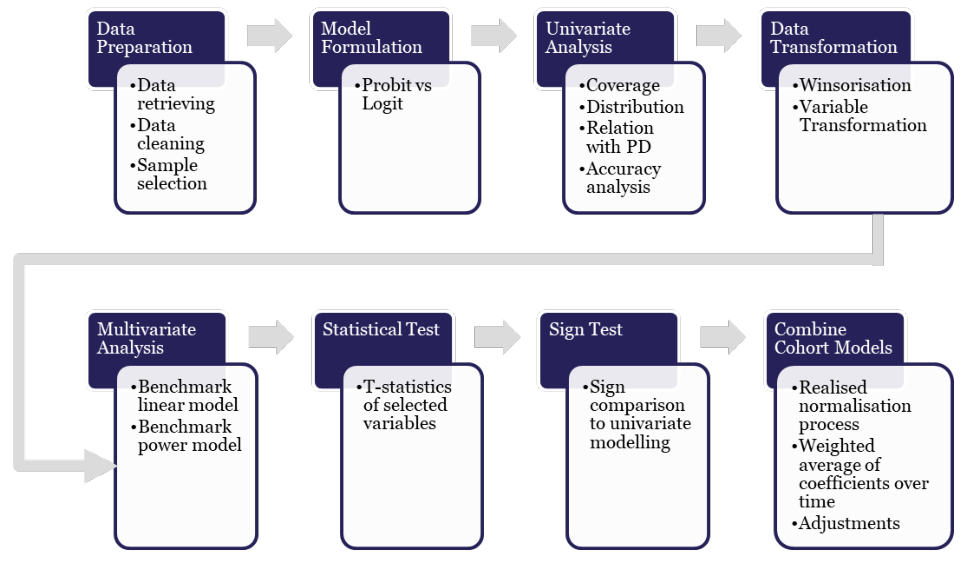
Note: This figure illustrates the general steps involved in the implementation of PuRA.
3.2 Data
Here we describe our data source for the example PuRA modelling exercise. The European Data Warehouse (ED) provides data warehousing services for loan level data of Asset-Backed Securities (ABS) transactions in Europe. The ED was established in 2012 as a part of the European Central Banks’s ABS Loan Level Data Initiative which aimed at standardising the data disclosure for ABS deals in the Eurosystem credit operations.
As of September 2018, the ED database covers 1219 deals covering 64.15 million loans and 54.85 million borrowers. The asset classes included in the ED database are RMBS, auto ABS, SME, consumer, leasing, credit card and CMBS. Figure 3 shows the distribution of the deals by asset class.
The ED 677 RMBS deals covers 15.67 million loans and 11.55 million borrowers. Figure 4 shows the country breakdown of the number of deals and number of loans respectively for the subcategory of RMBS deals.
We organised the RMBS data provided by the ED into a relational database. It was important to track the history of each individual loan across multiple snapshots of loan status and data provided by the ED. Figure 5 shows the breakdown of the number of loans that were performing at the beginning of each year by country and year. Figure 6 shows the breakdown by country and year of the number of loans that were performing in one year and then in default a year later. The default definition is consistent with the Basel definition of more than 90 days due or defaulted.
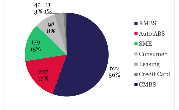
Note: This figure shows the distribution of the number of deals in ED database by asset class. The source is ED (2018).
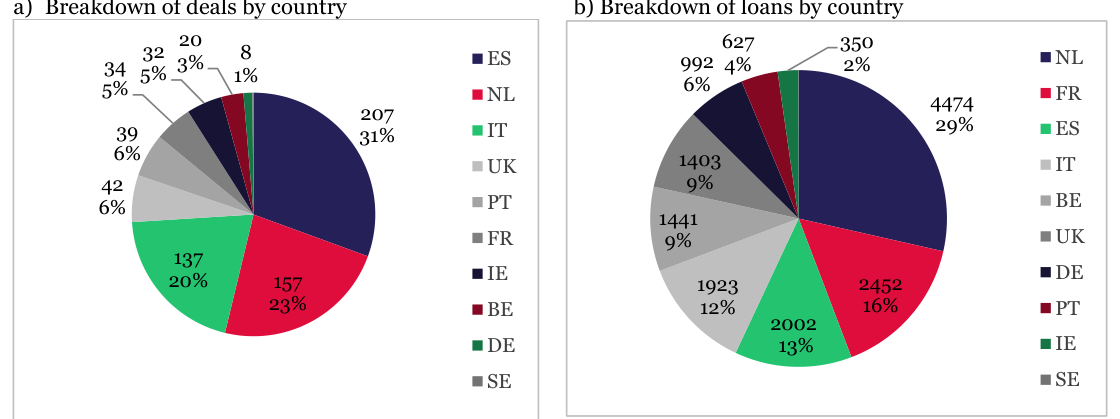
Note: The left hand panel shows the country breakdown of RMBS deals. The right-hand panel shows the country breakdown of loans in the corresponding pools. Number of loans expressed in 000s. The figures show ED has data for large number of deals for Spain, Netherlands and Italy. The individual loan data coverage is largest for Netherlands, France and Spain. The source is ED (2018).
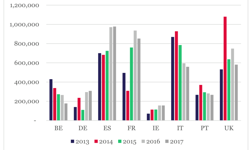
Note: This figure shows the breakdown of the number of performing loans at the beginning of each year by country and year. The source Risk Control calculations based on data provided by ED.
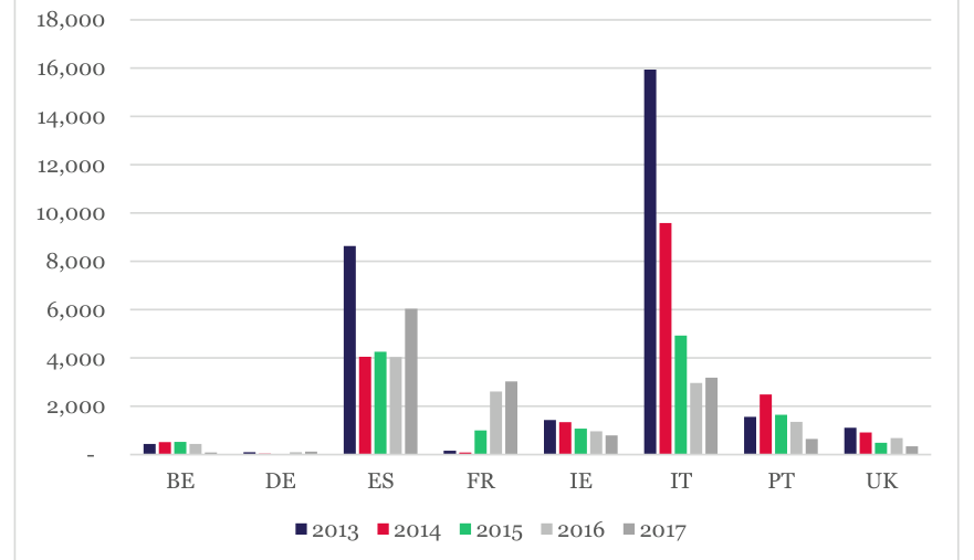
Note: This figure shows the breakdown of the number of defaulted loans by country and year. The source Risk Control calculations based on data provided by ED. This figure shows that the default observation count is largest for Italians and Spanish loans.
3.3 Results
This section presents the results for the PD and LGD models estimated using the ED data. We estimated PD models for eight individual countries employing all the useable observations available for the country in question. In each case, we employed as explanatory variables the debt to income ratio (x[1]) and the LTV ratio (x[2]) expressed in percentage. The fitted models for each country are presented below.
• PD model for BE
1 1 2 −β[3]x[2] y= c−β[1]x[1][3] −β[2]x[1] c= 6.32, β[1] = −5.47, β[2] = 2.77, β[3] = 0.03 (7)
• PD model for DE
y= c−β[1]x[1] −β[2]x[2] c= 8.33, β[1] = −0.06, β[2] = 0.01 (8)
• PD model for ES
y= c−β[1]x[1] −β[2]x[2] c= 7.4, β[1] = 0.09, β[2] = 0.04 (9)
• PD mode for FR
y= c−β[1]x[1] −β[2]x[2] c= 8.21, β[1] = 0.39, β[2] = 0.03 (10)
• PD model for IE
y= c−β[1]x[1]−3 −β[2] log(x[1]) −β[3]x[2] c= 3.44, β[1] = 0.03, β[2] = 0.03, β[3] = 0.004 (11)
• PD mode for IT
y= c−β[1]x[1] −β[2]x[2] c= 7.14, β[1] = 0.25, β[2] = 0.03 (12)
• PD model for PT
−3 −β[3]x[1] −1 −β[6]log(x[2]) y= c−β[1]x[1] −β[2]x[1] −1 −β[4]x[2] −β[5]x[2] c= 5.08, β[1] = 0.03, β[2] = 0.003, β[3] = 0.004, β[4] = 0.02, β[5] = −0.87, β[6] = −0.55 (13)
• PD model for UK
y= c−β[1]x[1] −β[2]x[2] c= 8.73, β[1] = −0.05, β[2] = 0.04 (14)
Note: This table presents the rank correlation between the estimated PDs and average PDs estimated from different country PD models based on country level data.
To understand how the models behaved differently across countries, we estimated PDs using each model for a set of 1000 randomly selected Spanish mortgages. By using the same loans and, therefore, the explanatory variables, we are able to focus on how the PD predictions of the models vary. Table 5 shows the results of this exercise for the models corresponding to the eight European countries. The table presents the correlation matrix of the PDs estimated using the different models and the average PD implied by each model. The results from Table 5 show that Spain and Portugal have the highest average PDs at 1.94% and 1.69% respectively. Germany is observed to have the lowest average PD of 0.06%.
Table 5 shows widely varying degrees of correlation between the PDs implied by the different models. PDs based on the UK model are strongly correlated with those implied by most of the other country models except those of Ireland and Italy. The Spanish and Portuguese model PDs are most closely correlated. PDs implied by the French model are somewhat lowly correlated with those from other countries.
We view these results not as serving as a basis for using a model based on one country’s mortgage loans to score the loans of another country. The structure and nature of these national mortgage markets and the approaches taken by the banks are too different. Our expectation is that a set of PuRA models will have at least one model per country for a given asset class.
To examine behaviour within a country, we focus on Spain. (We intend to look at additional countries and dimensions of variation but have not so far had time to pursue this.) We fit PD models to a set of Spanish datasets. These consist of all useable Spanish data (i.e., a country-level model), all data from individual Spanish banks (i.e., a bank-level model) and data from a single securitisation pool for a deal issued in 2013 (i.e., a deallevel model).
Table 6 shows the correlation matrix of the PDs and the averaged PDs estimated using these models.
Tables 7 shows the estimated models produced by using LTV ratio, debt to income ratio and smoothed odds ratio of loan origination year as explanatory variables.
Caja Rural de Caja Banco de Granada, ES Bancaja Madrid Valencia S.C.C. BBVA ES-deal LTV Ratio 0.04 0.04 0.05 0.05 0.05 0.03 0.001 Debt to Income Ratio 0.08 0.07 0.16 0.07 0.03 0.02 -0.11 Smoothed Odds Ratio of Loan Origination Year 0.49 1 1.17 0.8 0.7 1 1.47 0.83 Constant 7 .58 7 .69 11 7 .48 6.55 8.09 6.97 Turning to LGDs, we have estimated average LGDs by country but have not so far estimated defaulted-loanlevel regressions. Table 8 presents the count of default loans used for LGD calculation. The loan recoveries here satisfy Basel requirements in that it comes from the same mortgage loans for which we have identified default events.
We are aware that the data for several countries are scarce or indeed deficient. Most notably, the data for UK, Ireland and Germany are insufficient to produce reliable results. Clearly, more work would be necessary for these countries. For example, one could collect data directly from bank websites rather than from the ED. Some UK banks have offered to provide us with data to facilitate such an exercise but we have not so far been able to analyse them.
Table 9 presents the average LGDs estimated for the six European countries based on ED data alone. The LGD is calculated as the discounted loss divided by the default amount. If a particular loan returns to performing the LGD is set to 0. The LGDs for Italian and French loans are highest at 62% and 59%. The LGD for IE loans are the lowest at 13%. We have excluded UK and Germany due to the data deficiency.
The estimates in Table 9 underline the challenges. The range of estimates across countries does not align with prior expectations. The results for France and Ireland are, respectively, implausibly high and low. The challenges in calculating LGDs from public data might suggest that permitting banks to use regulatory LGDs would be advisable.
| BE | DE | ES | FR | IE | IT | PT | UK | |
|---|---|---|---|---|---|---|---|---|
| BE | 100 | 98 | 65 | 9 | 87 | 34 | 7 3 | 89 |
| DE | 98 | 100 | 7 0 | 15 | 89 | 40 | 7 8 | 93 |
| ES | 65 | 7 0 | 100 | 7 7 | 92 | 92 | 99 | 90 |
| FR | 9 | 15 | 7 7 | 100 | 52 | 96 | 69 | 46 |
| IE | 87 | 89 | 92 | 52 | 100 | 7 2 | 96 | 98 |
| IT | 34 | 40 | 92 | 96 | 7 2 | 100 | 86 | 67 |
| PT | 7 3 | 7 8 | 99 | 69 | 96 | 86 | 100 | 94 |
| UK | 89 | 93 | 90 | 46 | 98 | 67 | 94 | 100 |
| Mean PDs | 0.13% | 0.06% | 1.94% | 0.46% | 0.49% | 1.56% | 1.69% 0.27 | % |
| Caja | |||||||
|---|---|---|---|---|---|---|---|
| Rural de | |||||||
| Caja | Banco de | Granada, | |||||
| ES | Bancaja | Madrid | Valencia | S.C.C. | BBVA | ES-deal | |
| ES | 100 | 66 | 90 | 84 | 88 | 83 | 35 |
| Bancaja | 66 | 100 | 7 4 | 58 | 84 | 54 | 67 |
| Caja Madrid | 90 | 7 4 | 100 | 85 | 94 | 90 | 41 |
| Banco de Valencia | 84 | 58 | 85 | 100 | 7 8 | 7 4 | 14 |
| Caja Rural de Granada, S.C.C. | 88 | 84 | 94 | 7 8 | 100 | 87 | 54 |
| BBVA | 83 | 54 | 90 | 7 4 | 87 | 100 | 36 |
| ES-deal | 35 | 67 | 41 | 14 | 54 | 36 | 100 |
| Mean PDs 1.67 | % | 2.05% | 0.23% | 2.7 9% | 6.97 % | 1.7 5% | 0.26% |
Note: This table presents the rank correlation matrix of the PDs and the average PDs estimated using the models based on country level, bank level and deal level data. We estimated PD models for 5 Spanish banks: BBVA, Bancaja, Caja Madrid, Banco de Valencia, and Caja Rural de Granada SCC.
| Default | ||||||||
|---|---|---|---|---|---|---|---|---|
| year | BE | DE | ES | FR | IE | IT | PT | UK |
| 2013 | -- | -- | 10,338 | -- | 23 | -- | -- | -- |
| 2014 | 320 | -- | 2,368 | 131 | 526 | 924 | 223 | 114 |
| 2015 | 514 | -- | 942 | 114 | 639 | 1,544 | 434 | 98 |
| 2016 | 47 5 | -- | 953 | 114 | 341 | 1,038 | 383 | 92 |
| 2017 | 259 | 4 | 633 | 355 | 252 | 484 | 254 | 87 |
| 2018 | 9 | 3 | 17 5 | 400 | 21 | 209 | 17 4 | 2 |
| Total | 1,57 7 | 7 | 15,409 | 1,114 | 1,802 | 4,199 | 1,468 | 393 |
Note: This table shows the number of defaulted loans with valid loss data or recovery data or return to performing.

Note: The LGD is calculated as discounted loss/default amount. If the loan has returned to performing the LGD is set to 0.
4. IRB Models with an Inverted Data Hierarchy
4.1 Data hierarchy
Different IRB exercises, particularly those that rely on proxy data, require some combination of data. But the task of combining datasets becomes a central concern in the case of PuRA. The reason is that the usual data IRB hierarchy is inverted with the key data for calibration consisting of information about exposures closely related to the loan pool for which one seeks to estimate KIRB.
This means that instead of having a stable data source (such as a large volume of historical data on loans the bank has originated itself or some database provided by an external data vendor or data consortium), the modellers must use different datasets whenever they wish to calculate capital for a particular pool.
Thus, a PuRA model should be seen as a set of methodologies and procedures that are applied in a dynamic way to multiple deals as they arise and reapplied as long as the bank maintains its exposure to the positions in question. Such an approach must be sufficiently flexible that it is practical to apply to multiple, somewhat heterogeneous deals as they are presented to the bank. Yet, it must be sufficiently precise in formulation that regulators can be confident that the investor bank is approaching its securitisation risk in an orderly and prudent manner.
Figure 7 shows the data hierarchy that we envisage would actually apply for a bank implementing a PuRA model. At the bottom of the hierarchy is source 4 which consists of data on loans the bank has originated itself. Above that, we expect that the bank would access a ‘stable’ source of external securitisation pool data. This might take the form of loan level from the European Data Warehouse (ED). In some jurisdictions such as the UK, substantial volumes of data may be obtained from website maintained by large bank issuers (while data is also available from the ED). Also, data might be sought from other data providers like Intex. For this ‘stable’ external data, a distinction may be made between data from different originators (source 3) and data on loans issued by the originator of the deal in question (source 2). Lastly and at the top of the hierarchy is source 1 consisting of data directly relevant for the deal in question. If the loans are newly issued, performance data of the actual deal loans will not be available but the originator may possibly be able to supply data on closely comparable loans (which could be used in addition to the data from source 3).
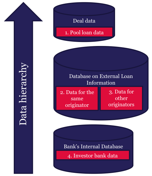
Note: This figure shows the different types of data a bank might employ while implementing rating system based on the PuRA.
4.2 Combining Data Sources
Given multiple datasets, the issue arises how in practice may a bank combine the information they each yield? One possibility would be to pool data from multiple sources. If this is done without some weighting in the combination will place a somewhat arbitrary emphasis on the different data sources and the results of the weighting will be opaque.
Potentially, models or forecasts may be combined using a formal statistical approach. Data is combined in some well-known area of risk management such as in the context of operational risk modelling. Typically, data from a small volume of internal loss observations is combined with a dataset obtained from a consortium of financial institutions. Guillen, Gustafsson and Nielsen (2008) present a model for operational losses that improves the internal loss distribution modelling by combining underreported internal and external data. Their model deals with the issue of combining data from different sources that have different collection threshold and reporting behaviours.[5]
Finally, Koh, Tan and Goh (2006) present data mining techniques for credit scoring and models and discuss how to combine these to obtain the best performance. Note that the models are assessed in their case by using combinations to score a single evaluation dataset. There is no similar evaluation dataset for the models that would be used in the combination required in a PuRA application.
Note that a broader statistical literature exists on combining forecasts from multiple models through so-called Model Averaging. The focus here, however, is not on different data sources but on applying different models to the same dataset.[6]
One useful way to combine information from different datasets is the method of “conflation” proposed by Hill
(2011) and Hill and Miller (2011). This method combines data from independent sources by consolidating a finite number of probability distributions, P[1], … , Pn into a single probability distribution denoted: &(P[1], … , Pn).
If the input distributions P[1], … , Pn have densities f[1], … , fn respectively, then the conflation &(P[1], … , Pn) is continuous with density given by:[7] f1(x)f2(x)…fn(x) f(x) = ∞ (15) ∫−∞f1(y)f2(y)…fn(y)dy
2, then the If P[1] and P[2] are two independent normal distributions with means μ[1] and μ[2] and variances σ[1][2] and σ[2] conflation &(P1,P[2]) is also a normal distribution with mean μ and variance σ[2] given by
μ1 σ12+μ2σ2 σ12μ2+σ2μ1 μ=[1] = (16) σ12+σ2 σ12+σ212
1 σ12σ2 σ[2] =[1] = σ[1][2]+σ[2][2]. (17) σ12+σ212
A number of papers use this method for combining datasets for a variety of applications. Touya, Coupé, Jollec, Dorie and Fuchs (2013) paper utilises conflation to combine geographic datasets. Principe et al. (2015) paper utilises the method of conflation for combining broadband thermal noise data.
In the case of PuRA, we can think of Pi(X)i=1,…,n as estimates of PDs for a given mortgage conditioned on mortgage characteristics described by a vector of variables X. The Pi (here suppressing the argument X) have a distribution fi reflecting sampling error and data quality issues. The may be biased estimates of the default probabilities of the pool loans in question in that they may be based on data for banks that apply different underwriting standards. To be prudent, a margin of conservatism (MoC) may also be employed.
Following the conflation approach, we would obtain an adjusted estimate of mortgage PDs based on the expression:
(18) P̃i = [Pi + biasadjustment(Pi) + MoC(Pi)]
Then, the final estimate might combine multiple PD estimates using the weighted average expression:
N Variance(Pi)P̃i ∑i=1 N 1 (19) ∑j=1 Variance(Pj)
Note that (18) includes a bias adjustment as well as a Margin of Conservatism (MoC). While the MoC as discussed in the EBA’s 2017 Guidelines does includes some allowance for underwriting standards, we interpret what is referred to there as an allowance for fluctuations in underwriting standards not an adjustment for a bias. In the context of PuRA, allowing for underwriting standards constitutes a central part of the modelling activity and represents more than just making an allowance for an additional source of noise or model risk.
Hence, we believe that it makes sense to make an explicit ‘bias adjustment’ for variation across banks and years in underwriting standards and then to reserve the term MoC for a buffer reflecting sampling errors or dataquality driven issues of parameter uncertainty. We discuss analysis of underwriting standards in the next section.
5. Adjusting for Underwriting Standards
Article 5 of the EBA draft RTS indicates that banks should reflect in their modelling variation in underwriting standards. This is challenging as empirical analysis of the effects on credit quality of underlying standards is limited.
Some academic studies have examined the issue. O’Keefe, Olin and Richardson (2003) study relationships between the riskiness of lending practices and subsequent changes in bank condition. They find that lower underwriting standards are generally associated with subsequent increases in nonperforming assets. Black, Chu, Cohen and Nichols (2012) find significant variations in the tendency to become delinquent depending upon whether a loan that was securitized into CMBS, was originated by a commercial bank, investment bank, insurance company, finance company, conduit lender, or foreign-owned entity. They argue that their results reflect the fact that the organizational structure of originators materially affects loan performance through their underwriting incentives.
Dell’Ariccia and Marquez (2006) suggest that, as banks obtain private information about borrowers and the information asymmetries across banks decrease, banks may loosen their lending standards. Asiedu, Freeman and Nti-Addae (2012) investigate discriminatory effects in the loan approval process. Their statistical exercise involves checking for robustness against differences and non-linearities in the underwriting standards of different lender types. Papers by Demyanyk and Van Hemert (2009) and An, Deng, Rosenblatt and Yao (2011) suggest the need to include cohort and cohort slope dummies in regressions in order to account for the effects of unmeasured changes in underwriting quality over time in the context of mortgage default risk.[8]
As well as the academic literature, official publications have focussed on underwriting standards. Financial Stability Board (2011) provides a thematic review of residential mortgage underwriting and origination practices. Subsequently, the FSB published a principles-based framework for sound underwriting practices. The Office of the Comptroller of the Currency (OCC) conducts annual surveys and assessments of credit underwriting standards and practices.
None of these papers provides what is necessary for PuRA modelling, however, which is a systematic analysis of how loans with identical performances vary in credit performance across countries, banks and origination years. Some investors we have encountered regard underwriting standards as more important in evaluating loan pools than the stage of the economic cycle and it is certainly the case that in certain European countries, loan pools issued under sound underwriting standards performed well even when loans originated by other banks experienced very poor credit outcomes.
Here, we sketch how, using the framework described in Section 3, we would go about analysing this issue. Given an extensive dataset of loan pool data such as we obtained from the European Data Warehouse (ED), one may estimate scoring models by country, bank, deal and origination year. We view the structure of the national mortgage markets that we have studies as so different that it is sensible to estimate models country by country. Within any given country, one may then estimate models by bank and origination year.
By including right hand side variables within a logit regression (for the PDs) or non-linear regression for the LGDs, one may allow for the fact that the composition of loans differs across banks and years. Differences in the average loan performance (in PD or LGD terms) for a given set of loans holding the right hand side variables constant, then reveals how much underwriting standards and macroeconomic conditions vary across banks. Variation across banks may be identified directly as an underwriting standard effect. Variation across time is more complex to interpret as it could reflect cyclical changes or changes in underwriting standards over time. Some judgment may be necessary to untangle these two influences. On the basis of the estimates and judgments, we would propose to develop bank and origination-year specific scaling factors for PDs. These would then be used to set the bias adjustments in equation (18).
6. Calculating Margins of Conservatism
As described in the EBA 2017 Guidelines (GL), the Margin of Conservatism (MoC) refers to the appropriate adjustments that an institution is required to incorporate in its estimation of the risk parameters in order to address any shortfalls in the estimation process.[9]
The EBA GL lists three broad categories of deficiencies that may occur:
• Category A: Identified data and methodological deficiencies;
• Category B: Relevant changes to underwriting standards, risk appetite, collection and recovery policies and any other source of additional uncertainty.
• Category C: General estimation error The final MoC is calculated as the sum of the MoCs under categories A, B and C[10] and is added to the best estimate of the risk parameter.
In our possible PuRA implementation approach (as described in equations (17) and (18)), we would seek to reflect these different influences in an estimate of the variances of the Pi estimates and then allow some prudent number of standard deviations as the MoC.[11] This short description leaves much to be settled as even calculating the effect of sampling error on Variance(Pi) is complex and demanding.
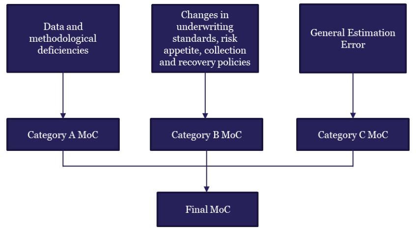
Note: This figure shows the different components of the MoC. The final MoC is obtained by taking the sum of MoC for categories A, B and C. Source is the EBA Guidelines on PD estimation, LGD estimation and the treatment of defaulted exposures.
7. Areas requiring clarification
The current draft RTS are helpful in clarifying a variety of issues including, for example, questions a bank may have about the operational requirements of the Purchased Receivables Approach (PuRA) as applied to securitisation exposures. Our focus in this paper is on the clarification that the RTS provide relative to the quantitative modelling tasks that banks will have to perform in implementing a PuRA model.
On this category of issues, we believe that the RTS have been useful in clarifying:
• That banks are eligible to seek permission to use a PuRA model for their securitisation exposures if they have an existing IRB permission in the regulatory relevant asset class.
• That regulators expect banks to develop a dedicated PuRA model rather than relying on an existing IRB model.
• That the usual IRB data hierarchy is inverted in the PuRA case.
• That the PuRA models should focus on variation in underwriting standards across originators.
However, some important issues affecting quantitative modelling aspects of PuRA remain less than fully clear and we would therefore suggest that the EBA provide further guidance on the following aspects:
• That PuRA models consist of methodologies that are applied in a dynamic way to different datasets as securitisation deals are presented to the bank. This appears to us a logical consequence of the inversion of the data hierarchy but we would like this to be confirmed.
• That banks may allow for underwriting standards by developing adjustments to PDs and LGDs based on analysis of how these quantities for mortgages with identical characteristics across (i) country, (ii) originator and (iii) period of origination.
• That Margins of Conservatism (MoCs) which will play a central role in PuRA modelling may be developed using quantitative analysis but with some element of prudent and evidence -based judgement.
We also believe that the EBA should be clear whether loan level analysis is essential or whether analysis based on aggregate performance measures (broken down by rep line or origination year) is acceptable. The latter approach is widely used by ratings agencies and securitisation market analysts.
8. Conclusion
This paper sets our responses to draft Regulatory Technical Standards (RTS) recently published by the EBA providing guidance to banks seeking to use the SEC-IRBA for calculating regulatory capital for banking book exposures to securitisations.
The RTS set out a number of requirements of banks using the SEC-IRBA, notably in their use of IRB models under the framework of the Purchased Receivables Approach (PuRA). Our focus in these comments is on the clarifications provided by the RTS on quantitative modellers within banks. We believe that the RTS are helpful in providing elements of a framework for PuRA modelling but that the guidance is overly concise and does not follow through on the logic of the points made.
First, PuRA modelling is very different from standard IRB modelling as it is implemented in many banks in Europe and elsewhere. IRB models are frequently very stable, being estimated off a stable dataset that may be periodically updated or even, in some cases, remains fixed in its estimation of relative credit quality rankings for some years. PuRA modelling in contrast consists of a dynamic activity in which modellers are authorised to develop a methodology that will be applied in an agile way to multiple datasets as and when deals are presented to an investor bank.
Second, the use of multiple data sources that is hinted at by the notion of an inverted data hierarchy suggests that banks will have to combine estimates of PDs and LGDs based on different datasets in potentially novel ways. In this paper, we sketch how this could be achieved but we believe that there is no guidance on this issue in the RTS and no usable information in the EBA’s 2017 guidelines on IRB modelling (GL).
Third, PuRA modelling requires a focus on differences in underwriting standards. The key significance of underwriting standards is familiar to those who take equity exposure to loan pools. The RTS emphasise in Article 5 the importance of modelling underwriting standards but provide few pointers as what is acceptable in this regard (beyond saying they should be regarded as a risk driver).
Fourth, Margins of Conservatism (MoC) discussed at some length in the EBA’s 2017 GL, would appear to be highly relevant for the PuRA. Yet, a fully statistical approach to the MoC in the PuRA case is highly challenging. Some recognition by the EBA that prudent, evidence-based MoCs with an element of judgments will be acceptable given the complex nature of the statistical task in formulating PuRA models.
Fifth, any bank implementing the PuRA will start with the issue of whether aggregate performance data (as standardly used for credit analysis by ratings agencies and used by investors to monitor deals) may subject to appropriate Margins of Conservatism be viewed as an acceptable basis for PuRA modelling or whether loan level analysis is required. To explain the point, starting from aggregate performance data, it is hard to track individual loans as is generally required in IRB modelling so that definitions of defaults and LGDs are consistent. Guidance from the EBA on this issue would be helpful.
9. References
An, X., Y. Deng, E. Rosenblatt and V.W. Yao (2012) “Model stability and the subprime mortgage crisis,” The Journal of Real Estate Finance and Economics, 45(3), pp.545-568.
Asiedu, E., J.A. Freeman and A. Nti-Addae (2012) “Access to credit by small businesses: How relevant are race, ethnicity, and gender?” American Economic Review, 102(3), pp.532-37.
Bank of England and European Central Bank (2014a) “The Impaired EU Securitisation Market: Causes, Roadblocks and How to Deal With Them,” Bank of England and European Central Bank Joint Statement, April, available at: https://www.ecb.europa.eu/pub/pdf/other/ecbboe_impaired_eu_securitisation_marketen.pdf?72fbdba6e14fbaa5d3497a4070e801ef
Bank of England and European Central Bank (2014b) “The Case for a Better Functioning Securitisation Market in the European Union: A Discussion Paper,” Bank of England and European Central Bank Joint Publication, May, available at: https://www.ecb.europa.eu/pub/pdf/other/ecbboe_case_better_functioning_securitisation_marketen.pdf
Basel Committee on Banking Supervision (2012) “Revisions to the Basel Securitisation Framework,” Consultative Document, Bank for International Settlements, December, (also known as BCBS 236), available at: http://www.bis.org/publ/bcbs236.pdf
Basel Committee on Banking Supervision (2013) “Revisions to the securitisation framework,” Consultative Document, Bank for International Settlements, December, (also known as BCBS 269), available at: http://www.bis.org/publ/bcbs269.pdf
Basel Committee on Banking Supervision (2014) “Revisions to the securitisation framework,” Basel III Document, Bank for International Settlements, December, (also known as BCBS 303), available at: http://www.bis.org/bcbs/publ/d303.pdf
Basel Committee on Banking Supervision (2017) “Basel III: Finalising post-crisis reforms, (also known as BCBS 424), available at: http://www.bis.org/bcbs/publ/d424.pdf
Board of Governors of the Federal Reserve System (2013), “Implementing the Supervisory Formula Approach for Securitization Exposures,” October, available at: http://www.federalreserve.gov/bankinforeg/basel/files/bcc1307.pdf
Black, L.K., C.S. Chu, A. Cohen and J.B. Nichols (2012) “Differences across originators in CMBS loan underwriting,” Journal of Financial Services Research, 42(1-2), pp.115-134.
de Jongh, R., T. Verster, E. Reynolds, M. Joubert, and H. Raubenheimer (2017) “A Critical Review Of The Basel Margin Of Conservatism Requirement In A Retail Credit Context,” The International Business & Economics Research Journal (Online), 16(4), p.257.
Dell'Ariccia, G. and R. Marquez (2006) "Lending booms and lending standards," The Journal of Finance, 61(5), pp.2511-2546.
Demyanyk, Y. and O. Van Hemert (2009) “Understanding the subprime mortgage crisis,” The Review of Financial Studies, 24(6), pp.1848-1880.
Duponcheele, G., W. Perraudin and D. Totouom-Tangho (2013a) “A Principles-Based Approach to Regulatory Capital for Securitisations,” BNP Paribas mimeo, April, available at: http://www.riskcontrollimited.com/wpcontent/uploads/2015/02/A_Principles-Based_Approach_to_Regulatory_Capital_for_Securitisations.pdf
Duponcheele, G. W. Perraudin and D. Totouom-Tangho (2013b) “Maturity Effects in Securitisation Capital: Total Capital Levels and Dispersion Across Tranches,” BNP Paribas mimeo, September, available at: http://www.riskcontrollimited.com/public/Maturity_Effects_in_Securitisation_Capital.pdf
Duponcheele, G., W. Perraudin and D. Totouom-Tangho (2014a) “Reducing the Reliance of Securitisation Capital on Agency Ratings,” BNP Paribas mimeo, February, available at: http://www.riskcontrollimited.com/wp-content/uploads/2015/02/Reducing_the_Reliance.pdf
Duponcheele, G., W. Perraudin and D. Totouom-Tangho (2014b) “Calibration of the Simplified Supervisory Formula Approach,” BNP Paribas mimeo, March, available at: http://www.riskcontrollimited.com/public/Calibration_of_SSFA.pdf
Duponcheele, G., A. Linden, W. Perraudin and D. Totouom-Tangho (2014c) “Calibration of the CMA and Regulatory Capital for Securitisations,” BNP Paribas mimeo, April, available at: http://www.riskcontrollimited.com/public/Calibration_of_CMA.pdf
Duponcheele, G., A. Linden and W. Perraudin (2014d) “How to Revive the European Securitisation Market: a Proposal for a European SSFA,” BNP Paribas mimeo, December, available at: http://www.riskcontrollimited.com/public/How_to_Revive_the_European_Securitisation_Market.pdf
Duponcheele, G., A. Linden and W. Perraudin (2015) “Comments on the Commission’s Proposals for Reviving the European Securitisation Market,” BNP Paribas mimeo, December, available at: http://www.riskcontrollimited.com/insights/comment-commission-proposals-securitisation/
Elul, R., (2015) “Securitization and Mortgage Default,” Working Paper 09-21R, Federal Reserve Bank of Philadelphia, May, available at: http://www.elul.org/papers/securitization.pdf
European Banking Authority (2014) “Discussion Paper on simple, standard and transparent securitisations,” (EBA/DP/2014/02), October, available at: https://www.eba.europa.eu/documents/10180/846157/EBA-DP- 2014-02+Discussion+Paper+on+simple+standard+and+transparent+securitisations.pdf
European Banking Authority (2015a), “EBA Technical Advice on Qualifying Securitisation”, Public Hearing Event, June, available at: https://www.eba.europa.eu/documents/10180/1116637/EBA+technical+advice+on+qualifying+securitisation +-Public+Hearing+Event+June+26+2015+%28final%29.pdf
European Banking Authority (2015b) “EBA Report on Qualifying Securitisation – Response to the Commission’s Call for Advice of January 2014 on Long-term Financing,” July, available at: https://www.eba.europa.eu/documents/10180/950548/EBA+report+on+qualifying+securitisation.pdf
European Union (2013) “‘Regulation (EU) No 575/2013 of the European Parliament and of the Council of 26 June 2013 on prudential requirements for credit institutions and investment firms and amending Regulation (EU) No 648/2012,” available at: https://eur-lex.europa.eu/legal-content/en/TXT/?uri=celex:32013R0575
European Union (2017) “Regulation (EU) 2017/2401 of the European Parliament and of the Council of 12 December 2017 amending Regulation (EU) No 575/2013 on prudential requirements for credit institutions and investment firms,” available at: https://eur-lex.europa.eu/legal-content/en/TXT/?uri=CELEX:32017R2401
European Banking Authority (2018) “Guidelines on PD estimation, LGD estimation and the treatment of defaulted exposures,” available at: https://www.eba.europa.eu/documents/10180/2033363/Guidelines+on+PD+and+LGD+estimation+%28EBA -GL-2017-16%29.pdf
European Banking Authority (2018) “Draft Regulatory Technical Standards on the conditions to allow institutions to calculate KIRB in accordance with the purchased receivables approach under Article 255 of [Regulation (EU) 2017/2401 amending Regulation (EU) No 575/2013],” June, available at: https://www.eba.europa.eu/documents/10180/2256128/Consultation+Paper+on+RTS+on+the+calculation+o f+Kirb+in+accordance+with+the+purchased+receivables+approach+%28EBA-CP-2018-10%29.pdf
European Data Warehouse (2018) “ABS Market Coverage – September 2018,” available at: https://eurodw.eu/wp-content/uploads/ABS-Market-Coverage.pdf
Financial Stability Board (2011) “Thematic Review on Mortgage Underwriting and Origination Practices: Peer Review Report,” March, available at: http://www.fsb.org/wp-content/uploads/r_110318a.pdf?page_moved=1
Financial Stability Board (2012) “FSB Principles for Sound Residential Mortgage Underwriting Practices,” April, available at: http://www.fsb.org/wp-content/uploads/r_110318a.pdf?page_moved=1
Fragoso, T.M., W. Bertoli and F. Louzada (2018) Bayesian model averaging: A systematic review and conceptual classification. International Statistical Review, 86(1), pp.1-28.
Guillen, M., J. Gustafsson and J.P. Nielsen (2008) “Combining underreported internal and external data for operational risk measurement,” available at: https://papers.ssrn.com/sol3/papers.cfm?abstract_id=1287068
Hansen, B.E. (2007) “Least squares model averaging,” Econometrica, 75(4), pp.1175-1189.
Hill, T.P. and J. Miller (2011) “How to combine independent data sets for the same quantity,” Chaos: An Interdisciplinary Journal of Nonlinear Science, 21(3), p.033102.
Hill, T. (2011) “Conflations of probability distributions,” Transactions of the American Mathematical Society, 363(6), pp.3351-3372.
Kaplan, D. and C. Lee (2018) “Optimizing Prediction Using Bayesian Model Averaging: Examples Using Large- Scale Educational Assessments,” Evaluation review.
Koh, H.C., W.C. Tan and C.P. Goh (2006) “A two-step method to construct credit scoring models with data mining techniques,” International Journal of Business and Information, 1(1).
Liu, C. and J.M. Maheu (2009) “Forecasting realized volatility: a Bayesian model‐averaging approach,” Journal of Applied Econometrics, 24(5), pp.709-733.
Moral‐Benito, E. (2015) “Model averaging in economics: An overview,” Journal of Economic Surveys, 29(1), pp.46-75.
Magnus, J.R., O. Powell and P. Prüfer (2010) “A comparison of two model averaging techniques with an application to growth empirics,” Journal of Econometrics, 154(2), pp.139-153.
Office of the Comptroller of the Currency (2016) “2016 Survey of Credit Underwriting Practices,” December, available at: https://www.occ.treas.gov/publications/publications-by-type/survey-credit-underwritingpractices-report/pub-survey-cred-under-2016.pdf
O'Keefe, J.P., V. Olin and C.A. Richardson (2003) “Bank Loan-Underwriting Practices: Can Examiners' Risk Assessments Contribute to Early-Warning Systems?”, available at: https://www.fdic.gov/bank/analytical/working/wp2003_06/wp2003_06.pdf
Perraudin, W. (2013) “Agency Cost Arguments for Non-Neutrality in Securitization Capital,” Risk Control 13- 81a 19-07-2013 v3
Perraudin, W. (2014a) “High Quality Securitisation: An Empirical Analysis of the PCS Definition,” July, available at: http://www.riskcontrollimited.com/wpcontent/uploads/2015/02/High_Quality_Securitisation.pdf
Perraudin, W. (2014b) “Quantitative Impacts of BCBS 269 Securitisation Capital Approaches,” Risk Control Limited Report, 14-73a, August, available at: http://www.riskcontrollimited.com/public/Quantitative_Impacts_of_BCBS_269_Securitisation_Capital_App roaches.pdf
Perraudin, W. (2015a) “Risk Control Comment on An EU framework for simple, transparent and standardised securitisation,” 15-53a Risk Control Limited Note, May, available at: http://www.riskcontrollimited.com/insights/consultation-eu-framework-securitisation/
Perraudin, W. (2015b) “Risk Control Comment on EBA Proposed Capital Rules,” 15-84a Risk Control Limited Note, August, available at: http://www.riskcontrollimited.com/wp-content/uploads/2015/09/Risk-Control- Comment-on-EBA-Proposed-Capital-Rules.pdf
Pesaran, M.H., C. Schleicher and P. Zaffaroni (2009) “Model averaging in risk management with an application to futures markets,” Journal of Empirical Finance, 16(2), pp.280-305.
Principe, M., I.M. Pinto, V. Pierro, R. DeSalvo, I. Taurasi, A.E. Villar, E.D. Black, K.G. Libbrecht, C. Michel, N. Morgado and L. Pinard (2015) “Material loss angles from direct measurements of broadband thermal noise,” Physical Review D, 91(2), p.022005.
Touya, G., A. Coupé, J.L. Jollec, O. Dorie and F. Fuchs (2013) “Conflation optimized by least squares to maintain geographic shapes,” ISPRS International Journal of Geo-Information, 2(3), pp.621-644.
Verma, V., F. Gagliardi and C. Ferretti (2009) “On pooling of data and measures,” Università di Siena, Dipartimento di metodi quantitativi.
Appendix: Data Quality
We employ loan level data on residential mortgages taken from the European Data Warehouse (ED) in this study. The data is delivered to the ED by individual banks. While the banks are supposed to adhere to ECB data definitions, there is considerable variation in the ways in which the banks interpret the definitions. Also, there are a significant number of cases in which the submissions of the reporting banks are subject to errors. Finally, use of the data is also complicated by different institutional features of national mortgage markets.
1. Some banks reported amounts in cents in some periods of 2013. Solution: If AR67(current balance) in Q1 2013 is 100 times of the amount in Q1 2014 we need to adjust the amounts reported in 2013 by dividing 100.
2. There are some 999 values. Solution: Check if there are any 999 values and replace with null.
3. BE data
i) Payment due data reported by Dexia in 2014 is 100 times or 10 times of the amount in 2013 and 2015. Solution: Divide payment due value by 100 or 10 ii) ING Belgium SA primary income data in 2014 is not consistent with 2013 and 2015. Solution: Replace 2014 primary income data with the average of 2013 and 2015 data
4. DE data
i) No default in 2015 ii) No PD model for 2015 iii) No primary income data for exposures in 2014 As we currently use LTV ratio and debt to income ratio (debt to income ratio=payment due/primary income) as the right-hand variables to fit the PD model, we are not able to fil a PD model if there is no primary income data. So no PD model for 2014. iv) Primary income data reported by Deutsche Bank PGK AG in 2016 is much lower than 2017 Solution: Deutsche Bank PGK AG started reporting from 2016, there is no way to replace 2016 income data with the average of 2015 and 2017. Simply replace the primary income data with 2017 data.
5. ES data
i) Santander deals report the loan balance in AR 67 until the number of months in arrears is 2, and from 3 onwards, they report the outstanding balance or the loan in the default amount field instead. Solution: In the LGD calculation, we use the default amount field if loan is in default (number of months is greater than 3). This issue won’t affect our calculation. There is no adjustment needed. ii) When BBVA deals report that a loan is 1 month in arrears, this means actually that the loan has crossed the 90 days already. For RURALPYME deals, there is the same issue as for BBVAs. Solution: Adjust number of months in arrears by adding 3.
6. NL data In Netherlands, for tax reasons, there are a lot of interest only loans (AR69 = 1) since the paid interest is tax deductible. Properties are therefore often financed with several loans, some amortizing, some interest only. Solution: Combine multi-loans financing the same property.
Risk Control 13-14 Dean Street London W1D 3RS +44(0)2033070730 www.riskcontrollimited.com
Notes
[1] See BCBS (2014) (also known as BCBS 303) for the Basel rules and European Union (2017) for the implementation of these rules in Europe in the form of the Capital Requirements Regulation (CRR).
[2] The Basel 3 rules involve a significant increase in conservatism comparted to the Basel 2 approach. While justified because of the role played by the subprime securitisations in the recent financial crisis, regulators have equivocated about whether the degree of the conservatism should be so great as effectively to preclude participation in the market by banks acting as investors. Early suggested rule changes such as BCBS (2012) and (2013) implied prohibitively conservative levels of capital. These proposals were extensively analysed in a series of papers on securitisation risk and capital, namely Perraudin (2013), (2014a), (2014b), (2015a), (2015b) and Duponcheele et al. ( (2013a) (2013b), (2014a), (2014b), (2014c), (2014d) and (2015). BoE and ECB (2014a) and (2014b) signalled in Europe a willingness to see the European securitisation revive at least in a modified form. EBA (2014), (2015a) and (2015b) developed modifications in capital rules for qualifying securitisations that would permit a partial revival for plain vanilla securitisations. The current EBA RTS specifying how European banks might use the SEC-IRBA by implementation of the PuRA is another step in facilitating the return of a prudent and stable level of securitisation activity in Europe.
[3] The operational requirements include monitoring the quality of securitized exposures and the financial condition of the institutions from which banks purchase the receivables. Legal requirements regarding ownership and control of the cash receivables must also be met. These requirements are described in an expanded form in Article 4.
[4] Such as that the pool is sufficiently granular. Note: This table summarizes the main regulatory requirements for developing an IRB PD model. Source is the Regulation (EU) No 575/2013 of the European Parliament and The Council of 26 June 2013 on prudential requirements for credit institutions and investment firms and amending Regulation (EU) No 648/2012. Note: This table summarizes the main regulatory requirements for developing an IRB LGD model. Source is the Regulation (EU) No 575/2013 of the European Parliament and The Council of 26 June 2013 on prudential requirements for credit institutions and investment firms and amending Regulation (EU) No 648/2012.
[5] Numerous other papers that deal with merging different datasets in other scientific disciplines. For example, Verma, Gagliardi and Ferretti (2009) discuss pooling of data over space and time from repeated multi-country surveys, taking illustrations from two major European social surveys. Ma and Bendersen (2014) present a statistical method for performing the joint analyses of multiple correlated astronomical data sets, in which the weights of data sets are determined by their own statistical properties.
[6] Fragoso, Bertoli and Louzada (2018) presents a review of trends in the development of Bayesian Model Averaging for application in model selection, combined estimation and prediction. Kaplan and Lee (2018) review Bayesian model averaging as a means of optimizing the predictive performance of common statistical models applied to large-scale educational assessments. Liu and Maheu (2009) paper presents a Bayesian model averaging approach applied to forecast realized volatility. Moral-Benito (2015) present a review of the literature on model averaging with special emphasis on applications to economics. Pesaran, Schleicher and Zaffaroni (2009) considers the problem of model uncertainty in the case of multi-asset volatility models and discusses the use of model averaging techniques as a way of dealing with the risk of inadvertently using false models in portfolio management. The Magnus, Powell and Prüfer (2010) paper presents a comparison of the Bayesian model averaging method with a Weighted-Average Least Squares (WALS) method. The authors argue that the WALS method is computationally less burdensome and is based on a more transparent definition of prior ignorance. Hansen (2007) discusses the WALS technique, selecting weights by minimizing a criterion based on the estimated average squared error from the model average fit.
[7] Here, it is assumed that the denominator equals neither zero nor infinity.
[8] In a related study not directly about underwriting standards, Elul (2015) compares the credit performance of US residential mortgages that were securitised and others that were retained on balance sheets and finds significant although not major differences in default rates.
[9] The notion of a Margin of Conservatism may of course be found earlier in Basel II. De Jongh et al (2017) list the various mentioned of conservatism and the MoC in the 2006 Basel II documents.
[10] Category A deficiencies includes issues such as missing, inaccurate or outdated default data, rating criteria and assignment, default triggers and future recoveries. It could also include issues related to inadequate data representativeness or bias arising from the choice of approach to calculating the average observed default rates. Category B deficiencies includes issues related to changes to underwriting standards, collection or recovery policies, risk appetite or other relevant internal processes, market or legal environment and unjustified deviations in the ranges of values of the key risk characteristics of the application portfolio compared with those of the dataset used for risk quantification. The MoC pertaining to general estimation errors are calculated to reflect the dispersion of the distribution of the statistical estimator. Category C deficiencies refers to sampling errors.
[11] How to estimate some components of the MoC is discussed in de Jongh et al (2017).