Hedging and Asset Allocation for Structured Products

Research Paper

Date:2005 Reference Number:5/2

HEDGING AND ASSET ALLOCATION FOR STRUCTURED PRODUCTS

Robert Lamb Vladislav Peretyatkin William Perraudin Imperial College Imperial College Imperial College, London London London

First version: September 2005 This version: December 2005∗

Abstract

This paper presents techniques for hedging structured products in incomplete markets. Under actual distributions, we simulate correlated ratings histories for pool exposures up to the hedging horizon and then employ conditional pricing functions estimated from a preliminary Monte Carlo based on risk adjusted distributions. The approach is very ﬂexible. We apply it to a realistic multi-period CDO transaction.

Keywords: Structured Products, Hedging, Pricing, Regression, Conditional Pricing Functions.

JEL classiﬁcation: D82, G13, C73.

1 Introduction

There is a substantial and growing literature on the valuation of structured products (see, amongst others, Li (2000), Duﬃe and Garleanu (2001), Hull, Predescu, and White (2005), Laurent and Gregory (2003) and the survey by Burtschell, Gregory, and Laurent (2005)). Less attention has been devoted to the hedging and asset allocation of these securities.

But, for many ﬁnancial institutions, controlling the risks they face in their structured exposure portfolios, either by hedging or suitable diversiﬁcation is an important priority. Anecdotes of ﬁnancial ﬁrms discovering that apparently low risk structured product exposures have suddenly become volatile as pool credit quality deteriorates are common. Perraudin and Van Landschoot (2004) show that investments in ABS behave very diﬀerently from those in standard bonds in that the former are more correlated and prone to episodes in which an entire market segment suﬀers a simultaneous fall in credit quality.

Analyzing risk and designing hedges for tranches of Collateralized Debt Obligations (CDOs) or Structured Products more generally is complicated by the fact that returns on such exposures depend in a complex way on (i) the performance of an underlying pool of assets, and (ii) the rules of the structured product waterfall. In eﬀect, they are highly non-linear functions of a large number of correlated state variables.

To analyze hedges or asset allocation decisions for structured product tranches is therefore a diﬃcult numerical task. In this paper, we describe a novel numerical technique that permits one to evaluate hedging strategies for individual structured products and to make asset allocation decisions for sets of exposures that include structured products.

Our approach involves estimating a statistical pricing functions for each individual tranche conditional on variables that describe the aggregate credit standing of the pool. Once these pricing functions have been estimated in a preliminary Monte Carlo, they are employed in a second Monte Carlo that yields risk measures such as volatilities and correlations with returns on other assets. Using these statistics, one may calculate Minimum Variance hedges and calculate mean-variance eﬃcient portfolios.

Our approach supplies accurate and stable estimates of appropriate hedges for a wide variety of structures with realistically complex cash ﬂow waterfalls. We illustrate its use for a CDO with a pool portfolio comprising 50 ﬁxed rate bonds and a waterfall structure that includes four tranches (one senior, two mezzanine and equity).

Our study may be related to several branches of the literature. First, numerous recent studies have investigated the modelling of correlated credit portfolios. General discussions may be found in Embrechts, Lindskog, and McNeil (2003), Frey and Mc- Neil (2003), and Kiesel and Schmidt (2004). Applications to CDO valuation include the studies cited above.

Most of these papers either discuss static, one-period models, or where a dynamic model is developed the approach taken consists of generating correlated times to default for the exposure in the pool (following Li (2000)). This latter approach to introducing dynamics has the disadvantage that it does not yield tractable conditional distributions as one steps forward in time so it is diﬃcult to investigate the behavior of prices and returns on tranches over multiple periods in a consistent fashion. One exception is Duﬃe and Garleanu (2001) which proposes a fully dynamic model of pool credit quality and pricing.

Our approach to simulating credit exposures resembles Duﬃe and Garleanu (2001) not in the detail of the modelling but in the one respect that it provides a fully dynamic framework. We simulate ratings changes for individual credit exposures period-byperiod into the future. Our model may be thought of as a multivariate version of the ratings-based credit derivative pricing models suggested by Jarrow, Lando, and Turnbull (1997) and Kijima and Komoribayashi (1998). Unlike these authors, we suppose that the risk-adjusted transition matrix for ratings is time-homogeneous. We incorporate correlation between rating changes for diﬀerent exposures by adopting the ordered probit approach that has become an industry standard in ratings-based credit risk modelling. See, for example, Gupton, Finger, and Bhatia (1997).

Our study is also related to the literature on hedging in incomplete markets as surveyed by Schweizer (2001). In this paper, we are mainly concerned with explaining how conditional pricing functions may be used in hedging and asset allocation of complex credit derivatives such as CDOs. We therefore take a simple approach to hedging in that we consider how positions in bonds may be used to oﬀset risk in

CDO tranches over a ﬁxed hedged horizon. Our hedging approach is therefore a static, one-period hedge designed to minimize the variance of the hedging error. We leave for future research the analysis of dynamic hedging over multiple periods as suggested in Cerny (2004) or issue of how static hedges can be implemented using multiple non-linear claims as in Carr, Ellis, and Gupta (1998).

2 Portfolio Modelling

2.1 Individual Exposures and Their Ratings Histories

In this subsection, we describe our approach to simulating dependent changes in the credit quality of simple exposures like bonds and loans. Consider a set of I such exposures denoted i = 1, 2, . . ., I. Suppose that, at date t, exposure i has a rating, Rit, which can take one of K values, 1, 2, . . ., K. Here, K corresponds to default, while state 1 indicates the highest credit quality category.

Since we wish both to price and to study the dynamics of ratings, we must distinguish between actual and risk-adjusted distributions of ratings changes. Assume that under both actual and risk-adjusted probability measures, Rit evolves as a timehomogeneous Markov chain. The actual and risk-adjusted K × K transition matrices are denoted: M and M∗ respectively. The (i, j)-elements of M and M∗ are mi,j and m∗i,j, respectively. Let mi,j,τ and m∗i,j,τ denote the (i, j)-elements of the τ-fold products of the matrices M and M∗, i.e., Mτ and (M∗)τ.

The actual transition matrix, M may be estimated from historical data on bond ratings transitions. We employ as our estimate the Standard and Poor’s historical, all-issuer transition matrix for the sample period 1970-2005 (see Table 1).

The risk-adjusted transition matrix M∗ may be deduced from bond market prices, in particular, from spread data on notional pure discount bonds with given ratings. To see how one may achieve this, note that if credit risk and interest rate risk are independent and spreads only reﬂect credit risk (i.e., there are no tax or liquidity eﬀects), the τ-maturity spread on a pure discount bond with initial rating i, denoted

Sτ(i), satisﬁes: exp −Sτ(i)τ = m∗i,K,τγ + (1 − m∗i,K,τ) . (1) where γ is the expected recovery rate in the event of default.

Let T ≡ τ[1], τ[2], . . . , τd denote a set of integer-year maturities. To infer the riskadjusted matrix, we may choose m∗i,j,t for i, j = 1, 2, . . .K − 1 and t ∈T to minimize: K−1 S(i) m∗ min τ − i,K,τγ + (1 − m∗i,K,τ) (2) m∗i,j,τ X X [2] . τ∈T i=1 Here, note that the m∗i,K,τ are implicitly functions of the mi,k∗ . (Note, we attach penalties to the objective function if entries in the transition matrix become negative in the course of minimization . This ensures the resulting risk adjusted matrix is well-behaved.)

In performing this calculation, we assume that the recovery rate γ is 50% and that the maturities in T are 1, 2, 3, 4, 5, 6, 7, and 8 years. The spread data we employ are time averages of pure discount bond spreads calculated by Bloomberg based on price quotes for bonds of diﬀerent ratings and maturities issued by industrial borrowers (see Table 2). The risk-adjusted transition matrix obtained in this way is given in Table 1.

2.2 Bond Ratings Histories and Values

The last section describes a theoretically consistent set of actual and risk-adjusted distributions governing the dynamics of ratings for our set of I exposures. Now consider how one may simulate changes in ratings building in dependence between ratings changes for diﬀerent obligors.

We employ the ordered probit approach widely used in ratings-based portfolio credit risk models. For any row of M (say the jth row), one may deduce a set of cutoﬀpoints Zj,k for k = 1, 2, . . ., K − 1 by recursively solving the equations:

= mj,1 Φ(Zj,1) mj,[2] = Φ(Zj,[2]) − Φ(Zj,[1]) ... ... ...

= (3) mj,K 1 − Φ(Zj,K−[1]) where Φ(.) is the standard normal cumulative distribution function. Doing this, we obtain a set of ordered cut oﬀpoints Zj,[1] ≤ Zj,[2] ≤ ... ≤ Zj,K−[1].

Given an initial rating j, to simulate a change in the rating from t to t + 1 for exposure i, we draw a random variable Xi,t+1. If Zj,k−[1] < Xi,t+1 ≤ Zj,k (where by convention Zj,[1] = −∞ and Zj,K = ∞), exposure i’s rating at t + 1 is k.

The latent variables Xi,t that determine changes in ratings are assumed to be standard normals. To include dependency between the ratings changes of diﬀerent exposures, assume that the Xi,t’s, for the exposures i = 1, 2, . . ., I, possess a factor structure, in that: J 1 − β[2] (4) Xi,t = q i X αi,jfj,t + βiǫi,t . j=1 Here, the fj,t are factors common to the latent variables associated with the diﬀerent credit exposures and the ǫi,t are idiosyncratic shocks. The fj,t and the ǫi,t are standard j=1 αi,jfj,t, is normalso standardand the weightsnormal. αi,j are chosen so that the factor component, PJ

If one knows the risk-adjusted probabilities of default for individual exposures and assumes that defaults, recovery rates and shocks to interest rates are independent, the valuation of individual exposures at some future date conditional on ratings is straightforward. For example, under these assumptions, the price Vt,R of a defaultable ﬁxed rate bond with initial rating R, coupons c, and principal Q is:

N = 1 − m∗ + γm∗ Vt,R c exp [−rt,t+ii] R,K,i R,K,i X i=1 . +Q exp [−rt,t+NN] 1 − m∗R,K,N + γm∗R,K,N (5)

It is simple to derive pricing Here, rt,t+i is the i-period interest rate at date t. expressions for ﬂoating rate loans and many other exposures including Credit Default Swaps (CDS), guarantees, letters of credit etc, under these assumptions as well.

Drawing together the various elements described above, one may simulate dependent ratings histories for all I exposures. The steps involved are:

1. Draw the fj,t and ǫi,t and calculate the latent variables for each exposure and each period using equation (4).

2. Deduce the time path followed by the ratings by comparing the latent variable realizations with the cut oﬀpoint intervals Zj,k−[1] < Xi,t+1 ≤ Zj,k.

3. Conditional on the rating at the chosen future date, price the I exposures.

4. Repeat the exercise many times to build up a data set of value and rating realizations.

2.3 Conditional Pricing Functions

The payoﬀon a structured exposure depends in a complex way on the performance of the pool of underlying exposures, typically bonds or loans. It is apparent from the above subsections how one may simulate the values of the individual exposures in the pool. To analyze hedging or asset allocation for a structured exposure, however, one must be able to simulate its price which is clearly much more complicated.

To put the task in context, one might consider simulating the underlying exposures up to the horizon of interest and then by simulating repeatedly from that date on, price the exposure at the hedge horizon through a Monte Carlo. This eﬀectively amounts to performing a pricing Monte Carlo for each replication of the initial hedge Monte Carlo. But, this approach is clearly infeasible however since it is computationally too costly.

Our alternative approach, which is much more eﬃcient computationally, consists of performing an initial valuation Monte Carlo (denoted Monte Carlo 1) that serves to estimate conditional pricing functions. These pricing functions are then used in a second risk management Monte Carlo (denoted Monte Carlo 2) in which we deduce appropriate hedges or analyze diﬀerent asset allocations.

To describe more precisely Monte Carlo 1 and the pricing functions it yields, consider, as before, a set of credit exposures, i = 1, 2, . . ., I with ratings histories Ri,t for t = 0, 1, . . ., T where T is the maturity date of the CDO.

For a given structure, we deﬁne the cash ﬂow waterfall to be a set of rules that determine the cash ﬂows to each tranche in the structure conditional on the evolution of ratings Ri,t for t = 0, 1, . . ., T and i = 1, 2, . . ., I.[1]

The waterfall rules may be described formally by a set of functions for dates t = 0, 1, 2, . . ., T that map the ratings histories up to t into cash ﬂows on the individual tranches, j = 1, 2, . . ., J, at that date:

= (6) cj,t Fj,t ({Ri,τ ; τ = 0, 2, . . ., t; i = 1, 2, . . ., I}) .

To estimate the pricing functions, we follow the steps:

1. Simulate correlated ratings histories starting from the initial values at t = 0 to the terminal date T . This simulation is performed using the ordered probit method described above but with the risk adjusted transition matrix, M∗, rather than the actual matrix, M.

2. Repeat the simulation M times. If c(j,tm) is the cash ﬂow in period t on tranche j in the mth simulation, we can deﬁne the summed discounted cash ﬂow at date t[1] (where 0 < t[1] < T ) on tranche j and for replication m, denoted DCFt,j,t(m)[1], as:

T DCFt,j,t(m)[1] = c(j,im)Pt,t[1],i. (7) X i=t[1]+1

Here, Pt,t[1],i is the forward discount factor at date t for discounting a cash ﬂow at date i back to date t[1]. The quantity DCFt,j,t(m)[1] in equation (7) is the cash ﬂows on a given tranche from t[1] onwards discounted back to that date using forward interest rates implied by the term structure at the initial date t.

3. We wish to obtain pricing functions for the tranches conditional on information at date t[1]. To represent that information, we deﬁne a set of S statistics h(t[1]m,s) (indexed s = 1, 2, . . ., S) of the individual obligor ratings Ri,τ up to the t[1] date.

h(t[1]m,s) = Ht[1],s ({Ri,τ ; τ = 0, 1, . . ., t; i = 1, 2, . . ., I}) s = 1, 2, . . ., S. (8)

The superscript m shows that statistic s is observed in simulation m. In principal, there are many variables observable at t[1] that one might expect would aﬀect cash ﬂows on the tranches subsequent to that date. A good example is the fraction of pool value in each of the rating categories at date t[1]. Such fractions are likely to be associated with systematically high or low outcomes for the subsequent cash ﬂows on the tranches.

4. To derive a pricing function, we regress the discounted, summed cash ﬂows DCFt,j,t(m)[1] on the information variables, ht([1]m,s). (The regression function we employ is more complicated than a simple linear regression. We discuss the regression we use in the next subsection.)

To understand why this yields a pricing function, suppose that t[1] = 0 and one performed a simple linear regression on a unit constant. This would be the same as averaging the discounted cash ﬂows DCF (m) t,j,t[1] over m. Given that the simulations have been performed using risk neutral distributions, this would yield an estimate of the price of the tranche at date 0 since we would simply be conducting a risk neutral Monte Carlo valuation of the claim.

By regressing the discounted summed cash ﬂows, simulated using risk neutral distributions on the information variables, we obtain a conditional pricing model. Evaluating the regression function at given levels of the information variables yields the prices of the tranche when the information variables take the values speciﬁed.

2.4 Estimating Conditional Prices

We described above how we derive a conditional pricing function by regressing the summed, discounted cash ﬂows on the information variables but were unspeciﬁc about what form the regression should take. In this subsection, we discuss for the form of the regression that it is advisable given the nature of payoﬀs on tranches.

In general, the regression model one employs should reﬂect the stochastic behavior of discounted payoﬀs on that tranche. Consider the density of discounted payoﬀs on a given tranche. A low credit quality tranche is likely to have an atom of probability associated with a zero payoﬀ. A very senior tranche may have an atom associated with full repayment (although even a senior tranche may have a state dependent payoﬀif poor performance of the pool triggers early substantial amortization). A mezzanine tranche may have atoms associated with zero payoﬀs and another associated with full repayment.

In light of this, we use diﬀerent regression functions for diﬀerent tranches depending on the number of replications in the Monte Carlo 1 for which the tranche in question either (a) defaults or (b) returns a zero discounted payoﬀ. We say that a tranche “defaults” if it pays less than the maximum contractual amount by the maturity date of the structure. (If a coupon payment is missed before this maturity date, the unpaid coupon is added to principal. A tranche is said to default if the full principal including unpaid coupons added to principal during the life of the structure cannot be fully paid at the maturity date.)

To be speciﬁc, a tranche is allocated to one of the following types of regressions depending upon its default behavior.

1. Equity Tranche A tranche is treated as an equity tranche if it is the most junior tranche in the structure or if it defaults more than 80% of the time. Equity tranches are valued using a linear regression of the discounted future payoﬀon the state variables. So the valuation expression is:

Equity value = Xtβ (9)

where β is a vector of regression coeﬃcients and Xt is a row vector of state variables.

2. Senior Mezzanine Variable Tranche A tranche is treated as a mezzanine variable tranche if it defaults more than 0.05% of the time and more than 10% of payoﬀs observations in the Monte Carlo diﬀer from the payoﬀin the previous replication. The pricing expression is:

exp (X′β[1]) Mezzanine variable value = Xtβ[2] + dtXtβ[3] 1 + exp (X′β[1]) 1 + exp (X′β[1]) (10) Here, β[1] is a vector parameter values for a logit model of the dummy variable that, for a given Monte Carlo replication, equals unity if the tranche defaults in the sense that it has a zero discounted payoﬀand otherwise is zero. The logit model is estimated by Maximum Likelihood. Xtβ[2] is the ﬁtted value from an ordinary least squares regression of the discounted tranche payoﬀs on the state variables, Xt, conditional on a default (in the sense just given) having occurred. dtXtβ[3] is the ﬁtted value from a linear regression of the discounted tranche payoﬀs on dtXt conditional on no default where dt is the outstanding par at the time of valuation.

3. Senior Mezzanine Constant Tranche A tranche is treated as a mezzanine variable tranche if it defaults more than 0.05% of the time and less than 10% of payoﬀs observations in the Monte Carlo diﬀer from the payoﬀin the previous replication. The pricing expression is:

exp (X′β[1]) Mezzanine variable value = Xtβ[2] + β[3],[0] 1 + exp (X′β[1]) 1 + exp (X′β[1]) (11) Here, β[1] is a vector parameter values for a logit model of the dummy variable that, for a given Monte Carlo replication, equals unity if the tranche defaults in the sense that it has a zero discounted payoﬀand otherwise is zero. The logit model is estimated by Maximum Likelihood. Xtβ[2] is the ﬁtted value from an ordinary least squares regression of the discounted tranche payoﬀs on the state variables, Xt, conditional on a default having occurred. β[3],[0] is mean of the discounted tranche payoﬀs conditional on no default.

4. Senior Variable Tranche A tranche is treated as senior variable if it defaults less than 0.05% of the time and discounted payoﬀs in successive Monte Carlo replications diﬀer more than 10% of the time. Such tranches are valued as:

Senior variable value = dtXtβ (12)

where dtXtβ is the ﬁtted value from a regression of the discounted payoﬀon dtXt.

5. Senior Constant Tranche A tranche is treated as senior constant if it defaults less than 0.05% of the time and discounted payoﬀs in successive Monte Carlo replications diﬀer on fewer than 10% of occasions. Such tranches are valued as:

Senior variable value = β[0] (13)

where β[0] is the mean discounted payoﬀ.

An important issue is: what “state” or “explanatory” variables should be included in the statistical pricing models? Examples of statistics that one may sensibly choose for the S(m) k,t[1] are the fractions of the value of the pool in diﬀerent rating categories and interest rate levels for diﬀerent maturities and exchange rates. If the model is simulated without interest and exchange rate risk, then the ratings fractions alone may be used.

3 Results

3.1 Example Structures

We consider a structure with a total pool par value of $65mn. The structure consists of: (i) a Senior Tranche with a par of $40mn, (ii) a Senior Mezzanine Tranche with par $20mn, (iii) a Junior Mezzanine Tranche with par of $2mn, and (iv) an Equity Tranche that has the residual claim.

The pool contains 50 bonds. Five bonds have a par of $6mn each and forty-ﬁve bonds have par equal to $0.875mn. We assume that there is a single risk factor and the correlation of latent variables for diﬀerent exposures is 0.2. (We also experimented with two risk factor portfolios but found results that were almost identical to the one-risk-factor case.) All bonds are rated BB.

We perform risk management simulations with a one-year holding period. When we perform Monte Carlos, we employ 200,000 replications.

3.2 On/OﬀBalance Sheet Comparisons

To assess whether the pricing functions are ﬁtting accurate conditional prices, we performed two exercises. In the ﬁrst, we ran a portfolio containing example CDOs (i) as described above. In this we assume that the investor is holding all four tranches of the deal. We estimate the conditional pricing functions in an initial Monte Carlo 1 and then in Monte Carlo 2 simulate the ratings up to a one-year horizon and then calculate the portfolio value using the conditional pricing functions.

In the second exercise, we suppose that the investor is holding the four tranches of the CDO as before but, in addition, has short positions in the underlying pool assets. Holding all the tranches should yield the same value as holding all the underlying assets, so an investment long in the tranches and short in the underlying assets should have zero value and volatility. Only if the conditional pricing functions are inaccurate would one ﬁnd that the hedged position was risky and had a mean far from zero.

The results of the two exercises are shown in Table 3. The mean value of the hedged position is $44,000 which is about 6 basis points of the value of the gross position in all the tranches ($65.09 million). The volatility of the hedged position is about a tenth of that of the unhedged position. The hedged position exhibits marked excess kurtosis but the VaR’s are about a twentieth of the magnitude of the VaR’s of the unhedged position.

These results are reassuring and suggest the conditional pricing functions, when evaluated at their rating-statistic arguments, are accurately mimicking the distribution of the tranche prices.

3.3 Hedging with Linked Bonds

We now turn to the ﬁrst substantive application of our methodology. Suppose an investor holds a CDO tranche and wishes to hedge it by trading in conventional bonds. These bonds might be claims of obligors whose debt is represented in the CDO pool (we refer to these as linked bonds) or they might be benchmark defaultable debt unconnected with the pool obligors (we refer to these as unlinked bonds). We investigate what bond holdings, the investor must acquire to implement a hedge that minimizes the variance of one unit of the tranche minus a hedge position.

We focus on CDOs with pools consisting of ﬁfty BB-rated or B-rated exposures of equal size. We consider the return variance-minimizing position made up of one unit of the tranche minus a hedge position in bonds issued by the same obligors as those represented in the pool (i.e., linked bonds).

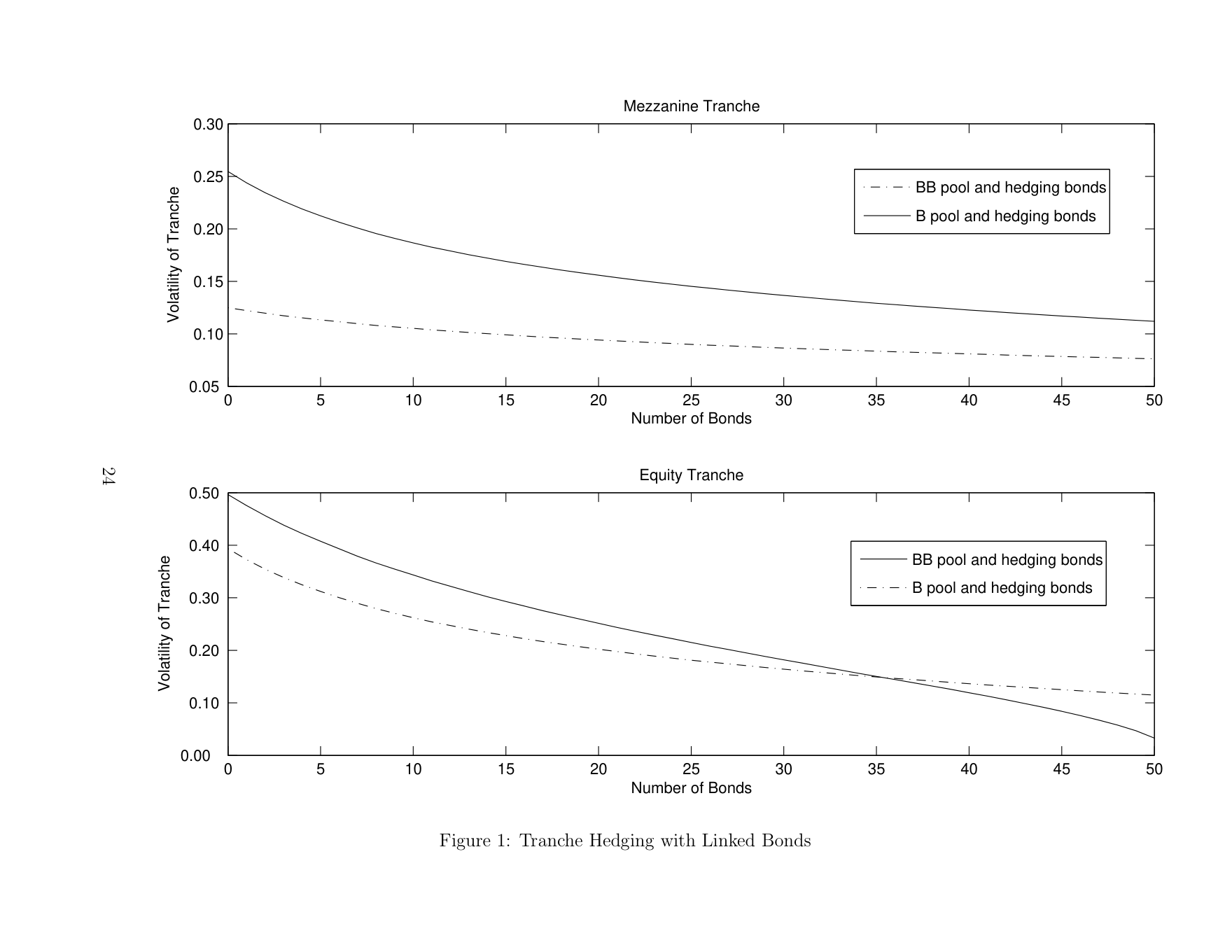
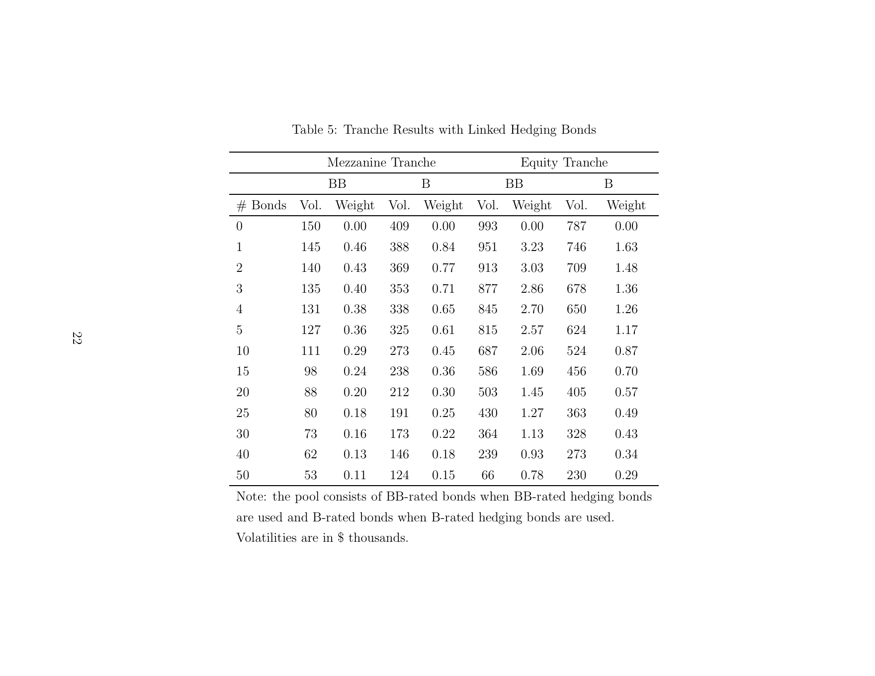
For CDOs with BB- and B-rated pools, Figure 1 and Table 5 show the volatility of the hedged net position (calculated using the the conditional pricing function approach) for the junior of the two mezzanine tranches and for the equity tranche. In each case the volatility is plotted against the number of bonds used in constructing the hedge.

The upper part of Figure 1 shows the volatility of the hedged mezzanine tranche payoﬀ. With no hedging, the volatility is 150 for the BB-rated pool transaction and 409 when the pool is B-rated. (Results here and in the tables are quoted in $ thousands.) When ﬁve bonds are employed the volatility drops to 127 and 325 for the two cases. When twenty bonds are used to construct a hedge, the hedged volatility falls to 88 for the BB-rated pool case and 212 in the B-rated pool case.

The lower part of Figure 1 shows the corresponding results for the equity tranche. When ﬁve bonds are used to hedge the equity tranche, the exposure volatility drops from the unhedged levels of 993 and 787 for the BB-rated pool and B-rated pool cases to 815 and 624 respectively. When twenty bonds are used for hedging, the payoﬀvolatility drops to 503 and 405 respectively.

3.4 Hedging with Unlinked Bonds

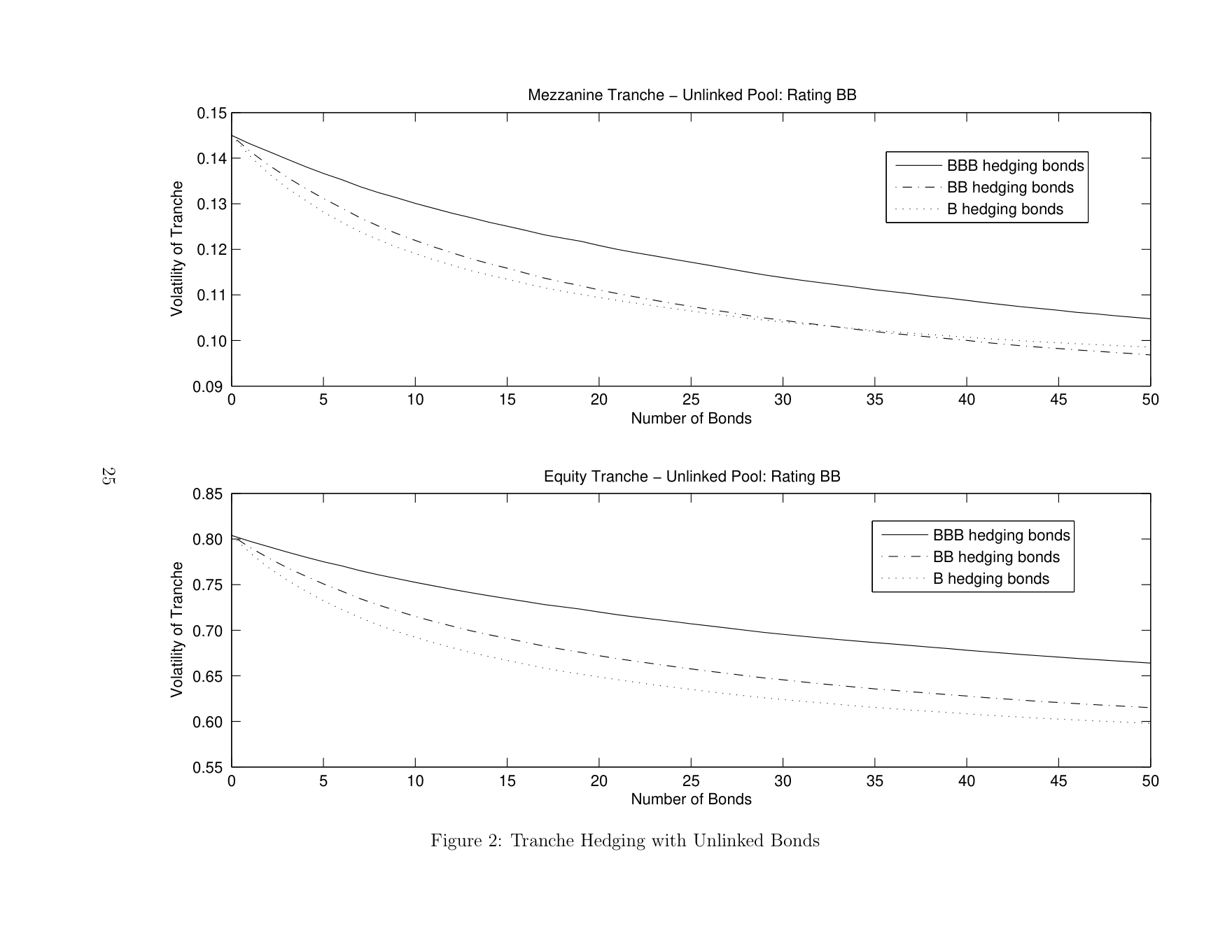
Hedging with linked bonds is likely to result in lower volatilities than hedging with unlinked securities. The reason is that unlinked hedging securities may assist in oﬀsetting factor risk in the structured product but introduce their own idiosyncratic risk.

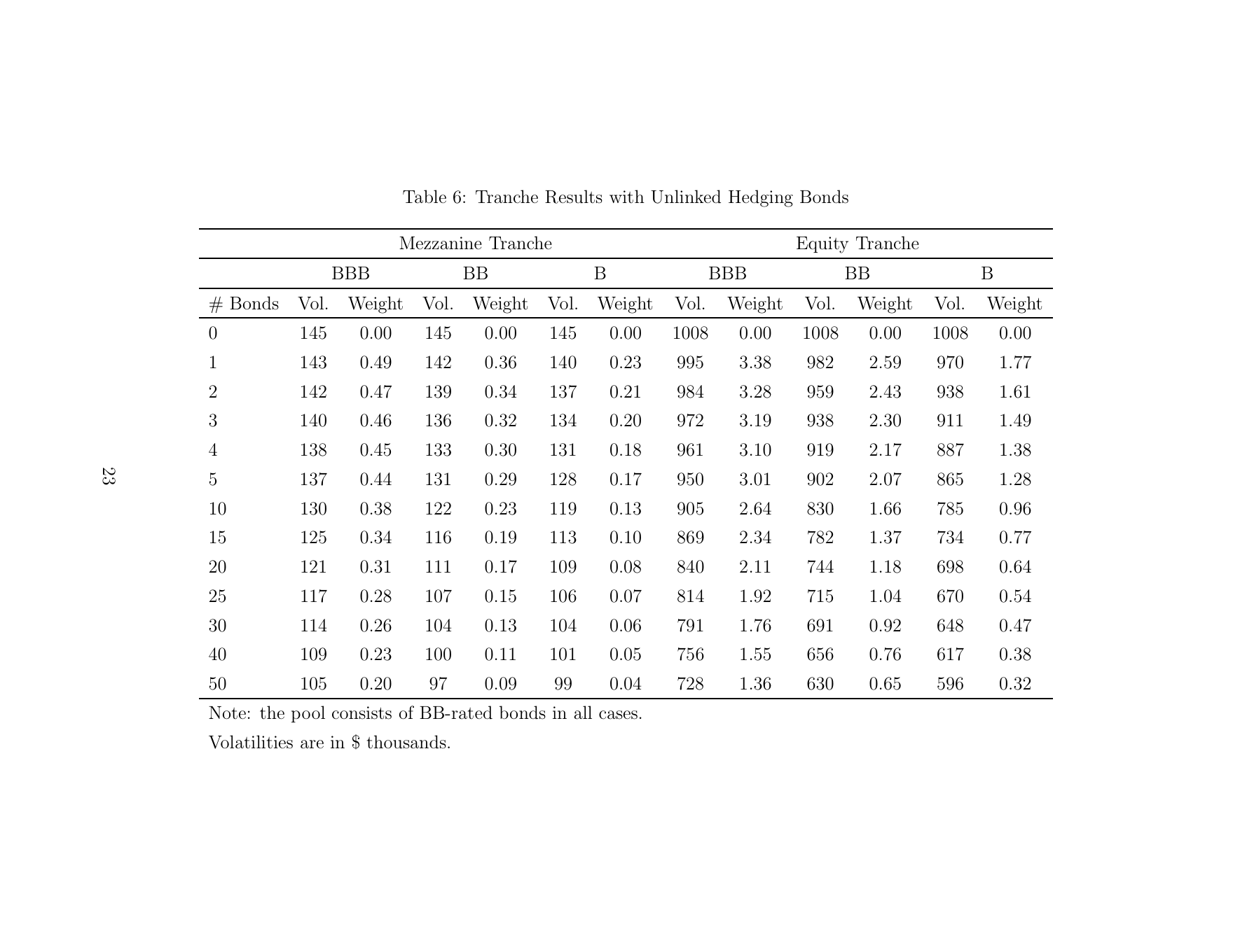
Figure 2 and Table 6 show results when unlined hedging bonds are employed. For the junior mezzanine and equity tranches, we report hedging results using BBB-, BB- and B-rated bonds. Volatility is reduced by hedging by between 30% and 40% depending on whether mezzanine or equity tranches are being hedged and on the rating of the hedging bonds. The best results are obtained in the case of equity tranche hedging using B-rated bonds.

3.5 Asset Allocation

The approach we have taken to designing hedges for CDO tranches, choosing the hedge to reduce volatility, immediately suggests extensions to mean-variance analysis and risk return tradeoﬀs. It is straightforward to calculate the mean-variance eﬃcient frontier for portfolios comprising bonds and CDO tranches using our approach and and this may be used to make decisions about asset allocation.

Figures 3 and 4 show eﬃcient frontiers for portfolios consisting of respectively (i) ten identical BB-rated bonds plus two mezzanine tranches and an equity tranche, and

(ii) ﬁve identical BB-rated bonds, bonds rated AA, A, BBB, B and CCC plus two mezzanine tranches and an equity tranche. The portfolio made up of the bonds and the tranches appears in the ﬁgures with the corresponding eﬃcient-frontier points (i.e., the point with the same volatility but higher mean and the point with same mean but lower volatility) also indicated.

The CDO tranches exhibit a quasi-linear trade-oﬀbetween volatility risk and expected return, with the senior mezzanine, having the lowest volatility and equity having the highest. In the case of the identical bonds (shown in Figure 3), the points corresponding to the identical bonds of course coincide and are further from the eﬃcient frontier than the points corresponding to the tranches.

In Figure 4, the diﬀerently rated bonds provide a wider dispersion of points as one would expect. The lower credit quality bonds appear with high volatility and vertically and horizontally far from the eﬃcient frontier.

4 Conclusion

This paper has described a fully dynamic credit risk model suitable for simulating portfolios of bonds and loans over multiple periods. We have described novel numerical techniques involving the development of conditional pricing functions which can be used to analyze consistently hedge positions in complex basket credit derivatives such as CDOs. Our study shows that hedges constructed with exposures to the names underlying the CDO may be used to reduce the return volatility of a CDO tranche position signiﬁcantly. Our hedging framework may be readily extended to analyzing asset allocation decisions involving CDOs, bonds and loans by calculation of eﬃcient frontiers.

References

Burtschell, X., J. Gregory, and J.-P. Laurent (2005): “A Comparative Analysis of CDO Pricing Models,” Working paper, BNP Paribas.

Carr, P., K. Ellis, and V. Gupta (1998): “Static Hedging of Exotic Options,” Journal of Finance, 53(3), 1165–1190.

Cerny, A. (2004): “Dynamic Programming and Mean-Variance Hedging in Discrete Time,” Applied Mathematical Finance, 11(1), 1–25.

Duffie, D., and N. Garleanu (2001): “Risk and valuation of collateralized debt obligations,” Financial Analysts Journal, 57, 41–59.

Embrechts, P., F. Lindskog, and A. McNeil (2003): “Modelling Dependence with Copulas and Applications to Risk Management,” in Handbook of Heavy Tailed Distributions in Finance, ed. by S. Rachev. Elsevier/North-Holland, Amsterdam.

Frey, R., and A. McNeil (2003): “Dependent Defaults in Models of Portfolio Credit Risk,” Journal of Risk, 6(1), 59–92.

Gupton, G. M., C. C. Finger, and M. Bhatia (1997): “Creditmetrics: Technical Document,” Discussion paper, J.P. Morgan, New York.

Hull, J., M. Predescu, and A. White (2005): “The Valuation of Correlation- Dependent Credit Derivatives Using a Structural Model,” Working paper, Joseph L. Rotman School of Management, University of Toronto.

Jarrow, R. A., D. Lando, and S. M. Turnbull (1997): “A Markov Model for the Term Structure of Credit Spreads,” Review of Financial Studies, 10, 481–523.

Kiesel, R., and R. Schmidt (2004): “A Survey of Dependency Modelling: Copula, Tail Dependence and Estimation,” in Structured Credit Products: Pricing, Rating, Risk Management and Basel II, ed. by W. Perraudin, pp. 3–34. Risk Books, London.

Kijima, M., and K. Komoribayashi (1998): “A Markov Chain Model for Valuing Credit Risk Derivatives,” Journal of Derivatives, 5(Fall), 97–108.

Laurent, J.-P., and J. Gregory (2003): “Basket Default Swaps, CDOs and Factor Copulas,” Working paper, ISFA Actuarial School, University of Lyon, Lyon.

Li, D. X. (2000): “On Default Correlation: A Copula Approach,” Journal of Fixed Income, 9, 43–54.

Perraudin, W., and A. Van Landschoot (2004): “How Risky Are Structured Exposures Compared with Corporate Bonds?,” in Structured Credit Products: Pricing, Rating, Risk Management and Basel II, ed. by W. Perraudin, pp. 283–303. Risk Books, London.

Schweizer, M. (2001): “A Guided Tour Through Quadratic Hedging Approaches,” in Option Pricing, Interest Rates and Risk Management, ed. by E. Jouini, J. Cvitanic, and M. Musiela, pp. 538–574. Cambridge University Press, Cambridge, UK.

Table 1: Transition Matrices

Historical* AAA AA A BBB BB B CCC D AAA 93.09 6.26 0.45 0.14 0.06 0.00 0.00 0.00 AA 0.59 91.06 7.54 0.61 0.05 0.11 0.02 0.01 A 0.05 2.10 91.49 5.61 0.47 0.19 0.04 0.05 BBB 0.03 0.23 4.34 89.22 4.64 0.92 0.28 0.36 BB 0.04 0.08 0.43 5.96 83.10 7.72 1.20 1.47 B 0.00 0.08 0.28 0.40 5.23 82.45 4.84 6.72 CCC 0.11 0.00 0.32 0.63 1.58 9.89 56.53 30.95 D 0.00 0.00 0.00 0.00 0.00 0.00 0.00 100.00 Risk-Adjusted† AAA AA A BBB BB B CCC D AAA 92.37 6.26 0.45 0.14 0.05 0.02 0.19 0.52 AA 0.59 90.58 7.53 0.59 0.01 0.02 0.06 0.62 A 0.06 2.10 90.47 5.60 0.43 0.18 0.36 0.81 BBB 0.08 0.27 4.37 88.35 4.52 0.72 0.49 1.21 BB 0.10 0.15 0.50 6.06 81.37 7.79 1.58 2.44 B 0.16 0.19 0.37 0.41 4.62 83.63 4.23 6.39 CCC 0.01 0.01 0.01 0.62 2.48 9.89 58.81 28.18 D 0.00 0.00 0.00 0.00 0.00 0.00 0.00 100.00 Note: entries are in %. * Source: Standard & Poor’s. † Fitted to spreads with maturities: 1, 2, 3, 4, 5, 6, 7, and 8 years.

Table 2: Spreads in Basis Points

Maturity AAA AA A BBB BB B CCC 1 26 31 41 60 123 325 1519 2 28 32 44 65 138 337 1289 3 29 33 47 70 150 342 1103 4 30 34 49 74 158 341 955 5 31 35 51 77 164 337 837 6 31 35 53 80 169 331 742 7 32 36 54 83 172 324 666 8 32 37 56 85 174 315 604

Table 3: On/OﬀBalance Sheet Results

Long structure Statistics short pool Long structure Mean value $ mn -0.044 65.69 Volatility of value $ mn 0.15 1.43 Skewness coeﬃcient 4.14 -2.71 Kurtosis coeﬃcient 41.26 13.62 Value-at-Risk 50bp, $ mn 0.34 6.68 Value-at-Risk 40bp, $ mn 0.35 7.05 Value-at-Risk 20bp, $ mn 0.39 8.22 Value-at-Risk 10bp, $ mn 0.42 9.36 Expected shortfall 50bp, $ mn 0.39 8.35 Expected shortfall 40bp, $ mn 0.40 8.72 Expected shortfall 20bp, $ mn 0.43 9.89 Expected shortfall 10bp, $ mn 0.45 11.06

Table 4: Statistics of Tranches

Mean Risk-free Volatility Exposure value value of value Senior tranche 40.00 40.00 0.00 Senior mezzanine 19.83 20.00 0.26 Junior mezzanine 1.83 2.00 0.18 Equity 4.08 3.00 1.06

Tranche Results with Linked Hedging Bonds

Tranche Results with Unlinked Hedging Bonds

Notes

∗The authors’ address is Tanaka Business School, Imperial College, London SW7 2AZ. Emails should be sent to rlamb@imperial.ac.uk, vperetyatkin@imperial.ac.uk or wper- raudin@imperial.ac.uk. 1The cash ﬂows may depend on a set of K other state variables (for example, interest rates or exchange rates) that we denote Skt for k = 1, 2, . . . , K. The may be introduced into the pricing functions without problem but we omit them here to simplify the notation.