

Abstract
This paper examines the effects of granularity and heterogeneity on capital requirements for securitisation transactions. For securitisation portfolios exhibiting a low number of obligors, a granularity adjustment to the Arbitrage Free Approach (AFA) (proposed by Duponcheele et al (2013a)) is derived in detail.
The adjustment is based on a second-order moment matching of the loss distribution under the Vasicek approximation. Capital based on the AFA inclusive of granularity adjustments is compared with the capital implied by a Monte Carlo model.
Similarly, for securitisation possessing heterogeneous pools (including barbell deals), the tranche capital implied by the AFA is compared with that obtained using a Monte Carlo model.
We conclude (i) that a simple version of the AFA, using pool level parameters, supplies accurate capital estimates even for extreme barbell deals, (ii) that the AFA, inclusive of granularity adjustments in the correlation, gives accurate capital measures for all except the few securitisation deals that have pools with fewer than 10 effective assets, and (iii) that for such deals, the AFA, inclusive of granularity adjustments to both the correlation and the lossgiven-default rates gives a capital distribution that is compatible with the situation in which recovery rates of individual assets are stochastic.
SECTION 1 – INTRODUCTION
The Arbitrage Free Approach (AFA) and Simplified Arbitrage Free Approach (SAFA) are detailed in Duponcheele et al. (2013a) and (2013b). Both are based on the Vasicek approximation for portfolio losses, as derived by Vasicek (2002). The simple Vasicek approximation is derived for homogeneous and infinitely grained portfolios. The approximation is the limiting distribution, which converges by the weak law of large numbers as the number of homogeneous obligors becomes arbitrarily large.
For the majority of underlying securitisation asset classes, particularly those with underlying retail exposures such as mortgages, consumer loans etc., the portfolio is granular enough for convergence of the approximation to hold without any adjustments. However, other types of securitisations with a lower number of distinct obligors, for example CMBS and some CLO securitisations, need special attention to compensate for the resultant lack of complete convergence of the approximation.
For non-granular portfolios, Vasicek (2002) proposes a granularity adjustment. This adjustment considers the non-zero second moment of the loss distribution, and uses secondorder moment matching to the granular case to arrive at a simple additive adjustment to the correlation. Since the moment matching does not consider higher order moments, and the matching of the second moment itself requires a further approximation[3], it is prudent to question how accurate the method is for realistic cases.
In its simplest form, the AFA is derived for securitisations possessing homogeneous pools of loans. A simple way of generalising the model to heterogeneous pools consists of calculating pool level inputs which are port-folio-share-weighted equivalents of the inputs for the model with homogeneous inputs. Again, it is an open question how accurate is this approximation.
In this paper, we evaluate the accuracy of different approximations within the AFA, with imperfectly granular and heterogeneous asset pools. We consider sequences of portfolios with decreasing granularity down to granularity level of 4 effective exposures. We also examine how pool level inputs perform (i) with extreme barbell pools and (ii) with pools that exhibit commonly observed probabilities of rating transition (having started with homogeneous ratings).
These issues are important because the Basel Committee’s recent proposals on capital for securitisations (See BCBS (2012), (2013a) and (2013b)), particularly as they relate to the Modified Supervisory Formula Approach (MSFA), make great play of the need to allow for imperfectly granular and heterogeneous pools. A question we seek to address here is whether an intrinsically simpler and more transparent approach, the AFA, can cope with the complications of imperfect granularity and heterogeneity.
The paper is organised as follows. Section 2 reviews the Vasicek loss distribution and the AFA. Section 3 considers the application of the Vasicek granularity approximation to the AFA and the SAFA. Section 4 compares the capital implied by the granularity adjusted AFA to the “true” capital implied by a Monte Carlo model. Section 5 discusses capital for deals with heterogeneous pools based on a version of the AFA with pool level inputs and on the Monte Carlo model. Section 6 concludes and an Appendix supplies a detailed step-by-step derivation of the Vasicek granularity adjustment.
SECTION 2 –REVIEW OF LOSS DISTRIBUTIONS AND THE AFA
In this section, we briefly review the Arbitrage Free Approach (AFA) proposed by Duponcheele et al (2012a).
The model is based on a simple two-factor formulation of the latent variables driving the credit quality of exposures in a securitisation pool. Suppose a pool of assets is securitised in an SPV (Special Purpose Vehicle). Assume that each individual loan defaults when a Gaussian latent variable falls below a threshold. We express the latent variables as:
(1) √ √ (2) √ √
In (2), is a factor common to all the exposures in the securitisation pool but is uncorrelated with the common factor driving the bank portfolio: .
Substitution yields:
(3) √ √ (4) √ (√ √ √ ) (5) ( )
We shall assume that the correlation parameter, , takes the value prescribed for exposures of this asset class by Basel II. If the latent variables of individual exposures within the pool have higher pairwise correlations than with those of exposures in the wider bank portfolio. Note that this two-factor, latent variable model is formally identical, under certain conditions on the correlation structure, to the Pykhtin-Dev model exposited in Pykhtin and Dev (2002) and (2003) and surveyed in Pykhtin (2004).
Consider a pool of one-year, homogeneous, infinitely granular, non-interest-bearing loans with individual default probabilities of , fractional expected losses of , and total par equal to unity held by an SPV. Suppose that the securitisation SPV has issued pure discount notes also with a total par value equal to unity. Suppose the notes consist of a continuum of thin tranches.
Under these assumptions, the expected losses of a discretely thick tranche with attachment point A and detachment point D equals:
1(− A)× ELSeniorTranche(A) − 1(− D)× ELSeniorTranche(D) ELThickTranche(A, D) = (6) D − A
where LGD× N[2] − X × PDTranche(X ) ELSeniorTranche(X ) = 1− X −1 −1 N[2] ≡ N[2] (N (PD), N (PDTranche(X )) , ρPool ) (7)
![Equation: −[1] −[1] X](/api/media/file/eq-92-300x30.png?prefix=media)
N (PD) − 1−ρ ⋅ N

LGD

PDTranche(X ) = N

ρPool

To calculate the marginal VaR (at an α-confidence level) of a thin tranche held within a wider bank portfolio, following the Gourieroux-Scaillet insight, one may calculate expected losses conditional on the common factor driving the bank portfolio, , equalling its αquantile.
Conditional on equalling its α-quantile, the default probability of individual pool exposures is: −1 −1

PDα= N (8)

1− ρ

Conditional on equalling its α-quantile, the pairwise correlation between pool assets is:
−1 Cov(Zi ,Z j | YBank = N ()α) * (9) ρPool,α ≡ −1 −1 = ρ σ(Zi |YBank = N ()α)⋅σ(Z j |YBank = N ()α)
Replacing and where they appear in equation (7) with and , respectively, yields expressions for the thin and thick tranche marginal VaRs.
SECTION 3 –GRANULARITY ADJUSTMENTS APPLIED TO THE AFA
The presentation of the AFA in the last section assumed a granular and homogeneous securitisation pool. Duponcheele et al (2013a) consider two ways of implementing the AFA, one based on pool-level inputs (their ‘Option 1’) and the other based on individual exposurelevel inputs (their ‘Option 2’). Both of these approaches may be adjusted for granularity. In the case of Option 1, one may employ the granularity adjustment suggested by Vasicek (2002). In the case of Option 2, the relevant granularity adjustment is slightly different.
In this section, we review in more detail the granularity adjustment relevant for Option 1 developed by Vasicek (2002) and then explain how granularity adjustments may be performed when Option 2 is employed.
Consider a portfolio of loans homogeneous in all aspects except their par values. Suppose they have weights in the portfolio summing to unity. Vasicek (2002) proposes a granularity adjustment based on a parameter, , defined follows:
∑ (10)
Let total portfolio losses be denoted, , where:
∑ (11)
Here, is an indicator variable, equalling unity when obligor i defaults and zero otherwise.
Following the derivation in Vasicek (2002), one may show that the variance of total losses equals:
(12) ( ) ( ( ) ( ) ( )) ( ( ))
One may fit the mean and variance of total losses with imperfect granularity to those that apply with perfect granularity by adjusting the latent variable correlation parameter, . This yields the granularity adjusted correlation parameter:
( ) (13)
Option 1 described in Duponcheele et al (2013) employs pool-level inputs. Calculating the parameter and then replacing correlation parameters where they appear in capital expressions with granularity-adjusted equivalents as in equation (13) yields a granularityadjusted version of the Option 1 AFA model.
As mentioned above, Duponcheele et al (2013) present an alternative approach to implementing the AFA, denoted Option 2, potentially applicable to deals with heterogeneous pools. Under Option 2, one implements the AFA by forming a theoretical pool consisting of notional assets identical to the consolidated sub-portfolio of exposures to the same obligor as asset .
If is the set of indices for exposures to the same obligor as exposure i, the portfolio weight, , for exposures to this obligor is:
(14) ∑
One may consider a notional portfolio of 1/ homogeneous, equally correlated obligors with correlation parameter: (assuming, for simplicity, that is an integer value). Then we have: (15) ∑ ∑
Hence, a slightly different granularity adjustment to the correlation is appropriate in this case, i.e.: (16) ∑ ( )
SECTION 4 –MONTE CARLO ANALYSIS OF GRANULARITY
In this section, we present comparisons of the capital implied by the Option 1 version of the AFA, inclusive of granularity adjustments, with the results of a Monte Carlo estimation of the “true” underlying capital charge. The Monte Carlo estimations may be regarded as an implementation of the ratings based model of portfolio risk proposed by J.P. Morgan (1997).
We examine two cases of imperfect granularity.
1. As a first exercise, consider an initial portfolio of 128 equally sized, homogeneous, 1-year loans. We create a sequence of securitisation pool portfolios by successively halving the number of exposures (while doubling their par values) until we arrive at 4 exposures. For each of the pools we consider (with 128, 64, 32, 16, 8 and 4 exposures), we compare the capital implied by the AFA inclusive of the granularity adjustment of Vasicek (2002) with ‘true’ values obtained from Monte Carlo estimation.
2. As a second exercise, we again consider a sequence of portfolios comprising two subportfolios of equal par value. The first sub-portfolio consists of 64 homogeneous loans. In the second sub-portfolio, an initial set of 64 loans is successively altered by halving the number of loans while doubling the par value until there remains a single dominant exposure. This exercise is motivated by the fact that the quality of approximation as convergence proceeds may be impaired by exposures that dominate the portfolio.[4]
In each of the two exercises, the rating of the underlying pool exposures is BB and the maturity of the pool exposures and structured exposures is one-year. Recovery rates are assumed to be constant and equal to 55%. In performing the Monte Carlo analysis, we suppose that each securitisation tranche that we are considering is held within a wider portfolio of 200 BBB-rated loans all with equal par values and maturities of 1 year. The number of replication completed in each Monte Carlo exercise is 5 million.
The securitisation pool is scaled so that its par value equals 7% of the par value of the onbalance-sheet loans. When we consider securisation tranches with 8 or fewer exposures, we reduce the relative size of the pool further, assuming that the par value of the pool is in that case 0.7% of that of the on-balance-sheet loans. We do this because otherwise the idiosyncratic risk of the individual pool loans could be significant to influence the estimated Unexpected Losses of the securitisation tranche exposures.
The calculations are performed using default probabilities implied by a rating transition matrix for US industrials reported in Standard & Poor’s (2008).
The pairwise correlations, denoted ρ, between the latent variables driving the credit quality of individual assets in the bank’s portfolio are given by the Basel formula. We assume that the * additional correlation between the latent variables for loans within the securitisation pool,ρ , is 10%. This is a reasonable benchmark value according to the calibration exercise reported by Duponcheele et al (2013a).
Table 1 shows the tranche structure of the securitisations we study. Below a single extremely thick tranche, we suppose there are 16 mezzanine tranches each comprising 2.5% of the total deal par value. Below the mezzanine tranches in seniority, we assume there are 10 junior tranches each with thickness equal to 1% of the total deal par.
Table 2 shows the total capital for all the tranches implied by the AFA model and the Monte Carlo approach. As one may observe, the AFA total capital is independent of the number of loans in the pool (and equal to KIRB, the capital the pool loans would attract if they were held on-balance sheet). This reflects the fact that the granularity of the pool is immaterial for total capital since the pool is assumed to be negligibly small compared to wider bank portfolio under the assumptions of the AFA. Granularity of the pool should only affect the distribution of capital across tranches of different seniorities, not the total level of capital allocated to all the tranches.
Also apparent from Table 2 is the fact that the Monte Carlo-based capital is slightly higher than the theoretical capital and gradually increases as granularity decreases. This reflects the fact that the Monte Carlo capital estimates are slightly boosted by idiosyncratic risk in individual loans that is only partially diversified away when the securitisation pool is assumed to be 7% of the bank’s wider portfolio and 0.7% when the pool contains 8 and 4 exposures.
Note that what limits scope for cutting the relative size of the securitisation pool further is that the precision of Marginal VaR and Unexpected Loss calculations is reduced when they become negligibly small. Hence, there is a trade-off between accepting (i) a slight upward bias through imperfect diversification and (ii) lower precision in the MVaRs and Unexpected Losses of each tranche. From looking at the distribution of capital across tranches of different seniority, it is important to have reasonably high precision in the MVaR and Unexpected Loss estimates.
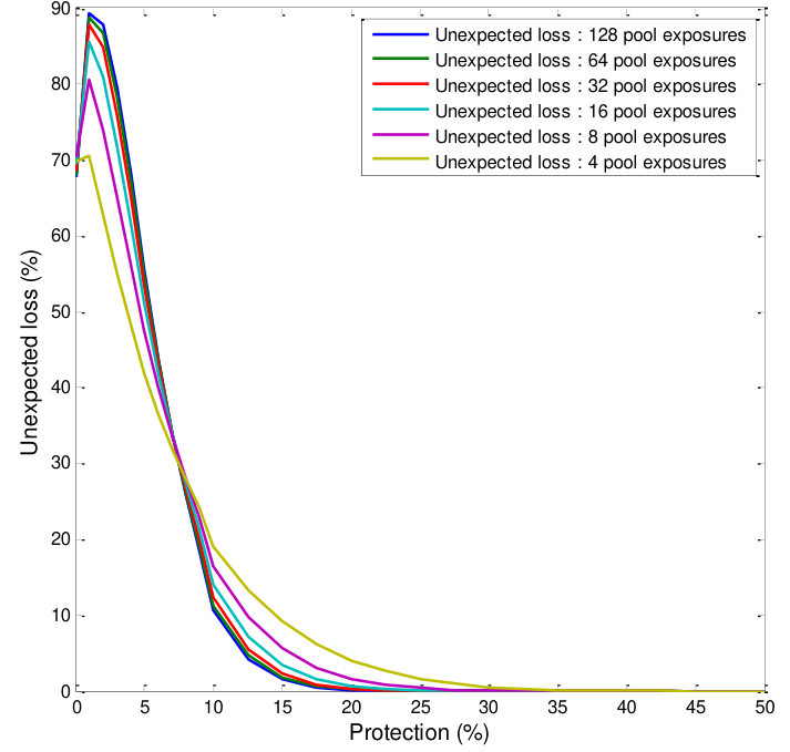
Figure 1 shows how the Vasicek (2002) granularity adjustments affect the distribution of Unexpected Loss-based capital across tranches of different seniority. As one may observe, the granularity adjustment shifts capital from the junior and lower mezzanine area towards senior and senior mezzanine tranches.
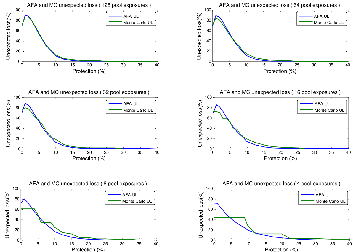
Figure 2 shows the same capital AFA-based capital inclusive of granularity adjustments and compares it to the capital implied by the Monte Carlo estimations. The six sub-plots corresponding to 128, 64, 32, 16, 8 and 4-loan pools show a good agreement between the two approaches for cases in which the number of pool exposures exceeds 16.
The assumption that we adopt in performing the Monte Carlo analysis of fixed recovery rates leads to flat areas in the Unexpected Loss plots in Figure 2 and makes it difficult to compare the compare the two sets of results in a meaningful way for very low granular pools. We could have assumed random recoveries in which case the Monte Carlo capital estimates would have appeared smoother but this would have introduced an inconsistency with the modelling assumptions employed in the AFA.
We believe it is fair to conclude from the comparisons that for granularity levels of more than 20 effective exposures, the AFA inclusive of Vasicek-style granularity adjustments provides a good approximation to the true capital that thin tranches of securitisations with imperfectly granular pools should attract. For thick tranches of securitisations, which correspond to reallife transactions, this number could be lowered to 10 effective exposures. The choice of 20 and 10 mentioned here are orders of magnitude rather than exact values.
When the granularity of the portfolio drops to very low levels, i.e. below 10, the effects of randomness in the loss given default of individual assets cannot be ignored. In Basel II, the LGD of an individual asset is not linked to the systemic risk factor when determining the Marginal Value at Risk. In consequence, only its mean matters for capital calculations. However, in the context of securitisations, randomness in recoveries alters the allocation of capital across tranches.
One may allow for this in the AFA by increasing the level of LGD where it appears in the AFA formulae. Specifically, one may replace the expression ( ) in equation (7) with a geometric interpolation ( ( )) where is the granularity parameter in equation (10). Illustrations of such adjustments are provided in Appendix 2.
Such an adjustment would lead to an increase in the amount of capital if the probability of default of the pool is not adjusted. In order to maintain the principle of neutrality, one should adjust the pool probability of default in equation (7) by multiplying it by ( ).
There are, of course, other solutions for dealing with the allocation of capital across tranches for those rare securitisations that exhibit very low levels of granularity. We intend to examine these alternatives in future work.
We now turn to the second exercise we perform to assess the accuracy of Vasicek-style granularity adjustments within the Option 1 version of the AFA. Recall that in this exercise, we consider a sequence of portfolios starting with 128 homogeneous pool exposures. To proceed along the sequence, we hold 64 of the 128 exposures unchanged which successively halving the number and doubling the par value of the exposures that make up the other half of the pool. In this way, we consider pools that contain 128, 96, 80, 72, 68, 66 and 65 exposures. In the 65 exposure pool, a single exposure has the same par value as all the rest of the exposures combined.
Table 3 shows the corresponding AFA and MC capital for all the tranches in the deal. Again, there appears to be some slight upward bias in the Monte Carlo estimates of total capital as the cost of achieving reasonable precision in the Unexpected Loss estimates for individual tranches.
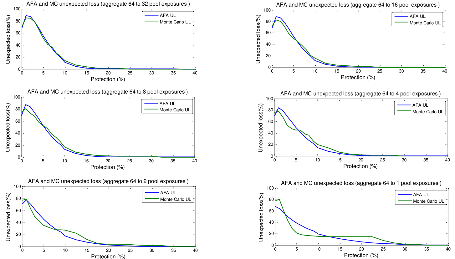
To save space, we do not present the equivalent of Figure 1 in this case but the effect of the granularity adjustment in the AFA is very similar in that capital is shifted from junior and junior mezzanine to senior and senior mezzanine tranches. Figure 4 shows the equivalent of Figure 2, i.e., a comparison of AFA capital for different tranches with the Monte Carloestimation-based capital for each of the different pool compositions assumed. In this case, the results suggest that the AFA supplies accurate capital values for portfolios of granularity equal or greater than the portfolio with 64 small and 8 concentrated exposures.
SECTION 5 –MONTE CARLO ANALYSIS OF HETEROGENEITY
In this section, we compare for heterogeneous pools the capital implied by the Option 1 version of the AFA with that obtained using the Monte Carlo approach described above. We examine two cases of heterogeneity.
1. In the first exercise, we consider a sequence of portfolios starting with 100 BBB-rated loans of equal par value. We work out, using a historical ratings transition matrix, the portfolio shares that the pool is likely to have in different rating categories after 1, 2, 3 and 4 years conditional on not defaulting. This provides an idea of how capital behaves as an initially homogeneous pool follows a ‘natural’ process of becoming more heterogeneous through the evolution of credit quality.[5]
2. In the second exercise, we examine a sequence of portfolios with different so-called ‘barbell’ structures. Specifically, we consider portfolios of 100 loans of equal par but with percentages 90% BBB-rated and 10% CCC rated, 80% BBB-rated and 20% CCC-rated and so on until we have a portfolio with 50% BBB rates and the remainder CCC-rated.
We begin by considering the first exercise. Table 4 shows the number of exposures in each rating bucket for the sequence of portfolios. Moving along the sequence, increasing numbers of exposures are in the ratings categories further from the initial rating of BBB.
Table 5 shows the total capital for all the securitisation tranches for the different deals. The total capital as measured by both the AFA and the Monte Carlo model increase as the distribution across ratings buckets increases. The growth is reasonably consistent across the two approaches.
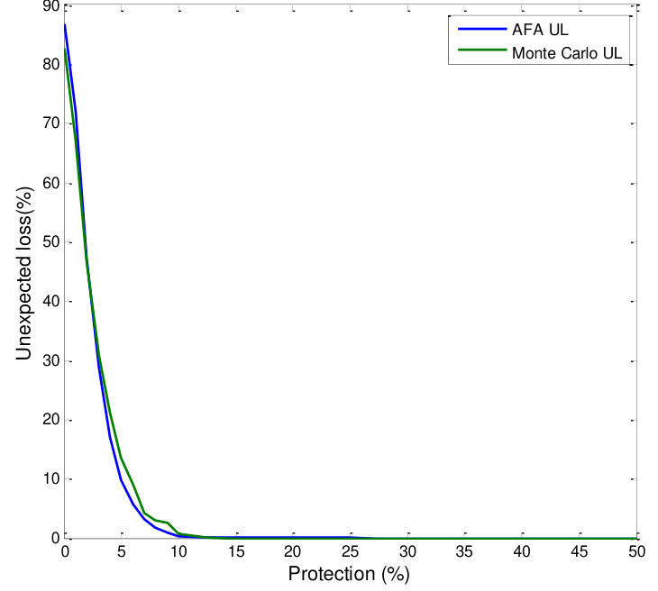
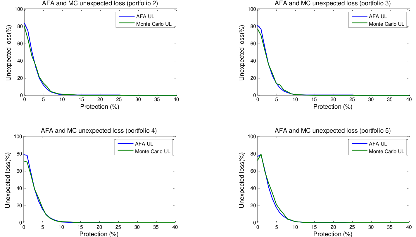
Figure 5 shows the capital implied by the AFA and the Monte Carlo-based capital estimates for portfolio 1, i.e., the case in which all the loans are rated BBB. Figure 6 shows the results for portfolios 2, 3, 4 and 5, corresponding to cases in which the pool ratings have evolved to equal those that would be implied by the natural evolution of the ratings starting at BBB after 1, 2, 3 and 4 years. It is striking how closely the AFA capital shown in Figure 6 matches the capital implied by the Monte Carlo estimates.
We now turn to the second heterogeneity exercise. Recall that this involves calculating capital for a sequence of portfolios, each consisting of 100 1-year maturity loans. The loans are split into BBB- and CCC-rated categories as shown in Table 6. Table 7 shows the total Unexpected Loss (UL) and the total Expected Loss (EL) implied by the AFA under Option 1 and by the Monte Carlo estimates for each of the portfolios.
One may observe that the total ELs implied by the two approaches are almost exactly equal while the total ULs are very good approximations. This is perhaps not surprising since despite the barbell nature of the portfolio, the capital implied by the AFA equals the capital attracted by the underlying pool, KIRB, which is the theoretically correct under these assumptions.
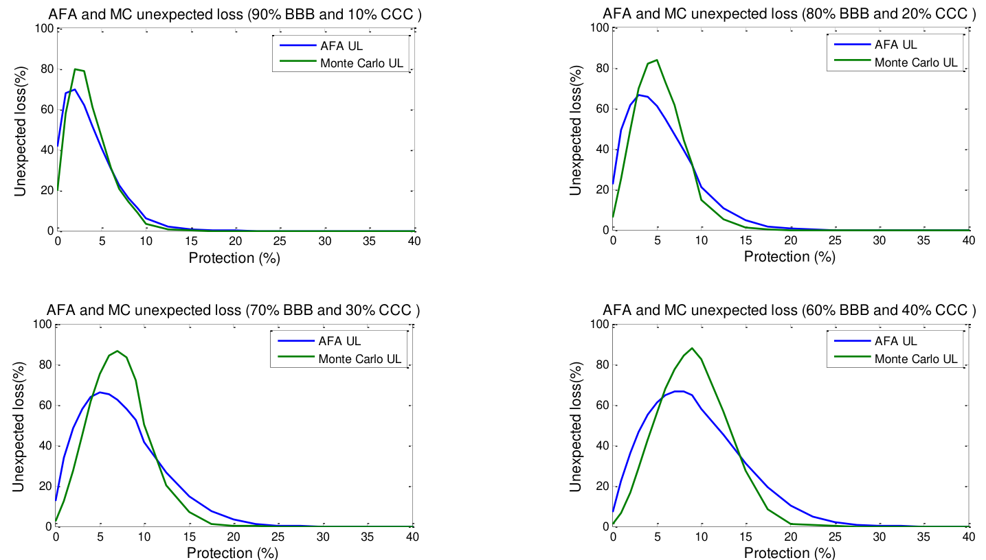
The distribution of capital across tranches implied by the Option 1 AFA and by the Monte Carlo approach is shown for portfolios 2, 3, 4 and 5 in Figure 7. As one may observe, from Figure 7, the distribution of capital implied by the AFA is a reasonable approximation to that yielded by the Monte Carlo approach even in these cases of barbell portfolios. There are some regions of the mezzanine area of the deals in which the Monte Carlo capital exceeds that implied by the AFA. The AFA capital is more conservative for senior tranches and junior mezzanine tranches on the other hand.
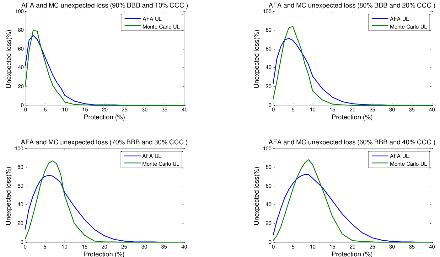
One way to mitigate the fact that the AFA is less than completely conservative for tranches in a particular range of seniorities (although it is more conservative than the Monte Carlo approach in other ranges) is just to increase the conservatism of the approach globally. Figure 8 shows the distribution of capital implied by the AFA if its KIRB input is boosted by 20%. (One might note that the first Basel Working Paper on securitisation capital (see BCBS (2001)) suggested that capital after securitisation should equal 20% more than capital prior to securitisation.)
As shown in Figure 8, the boost of 20% in the KIRB input has the effect of increasing capital for tranches throughout the seniority range. This reduces the area of seniorities in which the AFA is less conservative than the Monte Carlo estimates.
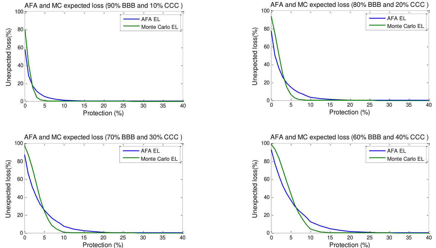
Lastly, in Figure 9 we show the distribution of Expected Losses (EL) for tranches of different seniorities. One may observe discrepancies between the Option 1 AFA ELs and the Monte Carlos-based ELs. In particular, the AFA is much more conservative about the levels of ELs experienced by senior tranches in the structures. However, the curves may be viewed as reasonable approximations. For capital rules that involve deduction for more junior tranches, being more conservative for senior and less conservative for junior tranches is not a serious failing.
Overall, we think it is reasonable to conclude from the above analysis that the Option 1 AFA performs very well in approximating the ‘true’ capital levels implied by the Monte Carlo estimates. Even in the case of barbell portfolios, the Option 1 AFA appears to be a reasonable and appealing simple way to calculate capital.
SECTION 6 –CONCLUSION
This paper has investigated the effects of granularity and heterogeneity on the appropriate capital for securitisation tranches. We do this by comparing capital implied by the Arbitrage Free Approach (AFA) of Duponcheele et al (2013a) with capital estimates based on Monte Carlo estimations. The AFA model allows for granularity by including an adjustment to correlation and can be implemented for deals with heterogeneous pools by use of pool-level inputs such as KIRB and weighted averages of other parameters such as LGD.
For the 1-year maturity deals on which we focus, the total capital for all the tranches in a securitisation should under our assumptions equal the on-balance sheet capital given by the Basel notion of KIRB. Unsurprisingly, we find close correspondence between total capital measured by the two approaches.
We find that the granularity adjustments in Option 1 of the AFA which are based on Vasicek
(2002) perform well for portfolios with more than 10 effective assets in that the AFA capital distribution and that implied by the Monte Carlo estimates are very similar. For the rare situations of less than 10 effective assets, we find that an additional granularity adjustment to the LGD yields reasonable results.
The AFA also yields accurate approximations to the ‘true’ distribution of capital for the heterogeneous pool deals we examine. This is particularly the case for the ‘natural’ heterogeneity one observes in deals that start homogeneous but become heterogeneous as the credit quality of the pool evolves over time. Even for so-called barbell pools, the AFA seems to offer a reasonable approximation to the capital implied by the Monte Carlo.
| Percentage | Number of | |
|---|---|---|
| Category | of total par | tranches |
| Junior tranches | 10% | 10 |
| Mezzanine tranches | 40% | 16 |
| Senior tranches | 50% | 1 |
| Total | 100% | 27 |
| of | ||
|---|---|---|
| pool AFA | total | |
| capital MC | capital | |
| 128 | 6.13% | 6.28% |
| 64 | 6.13% | 6.32% |
| 32 | 6.13% | 6.52% |
| 16 | 6.13% | 6.36% |
| 8 | 6.13% | 6.64% |
| 4 | 6.13% | 6.77% |
| Aggregated | ||
|---|---|---|
| pool AFA | total | |
| exposures | capital MC | capital |
| 32 | 6.13% | 6.28% |
| 16 | 6.13% | 6.27% |
| 8 | 6.13% | 6.48% |
| 4 | 6.13% | 6.42% |
| 2 | 6.13% | 6.63% |
| 1 | 6.13% | 6.42% |
| Portfolio | 1 Portfolio | 2 Portfolio | 3 Portfolio | 4 Portfolio | 5 |
|---|---|---|---|---|---|
| AAA | 0 | 1 | 1 | 1 | 1 |
| AA | 0 | 1 | 1 | 1 | 1 |
| A | 0 | 3 | 7 | 10 | 13 |
| BBB | 100 | 90 | 81 | 75 | 69 |
| BB | 0 | 3 | 7 | 10 | 12 |
| B | 0 | 1 | 2 | 2 | 3 |
| Cs | 0 | 1 | 1 | 1 | 1 |
| Total | 100 | 100 | 100 | 100 | 100 |
| AFA | capital MC | capital | |||
|---|---|---|---|---|---|
| Portfolio | 1 | 2.75% | 2.83% | ||
| Portfolio | 2 | 2.91% | 2.83% | ||
| Portfolio | 3 | 3.05% | 2.98% | ||
| Portfolio | 4 | 3.18% | 3.04% | ||
| Portfolio | 5 | 3.30% | 3.47% | ||
| 5 | |||||
| Mathematically, | the | portfolio shares are | derived for | portfolios 2, 3, 4, and 5 in the | sequence |
| BBB row in | the historical | transition matrix | taken to the | powers 1, 2 , 3 and 4, deleting | the last |
| row and then | dividing the | remaining elements | by their | sum so the final weights sum | to unity. |
| 6 | |||||
| The AFA | capital increases | with the maturity | due to | the IRBA maturity adjustment. |
| Portfolio | 1 Portfolio | 2 Portfolio | 3 Portfolio | 4 |
|---|---|---|---|---|
| BBB | 90 | 80 | 70 | 60 |
| CCC | 10 | 20 | 30 | 40 |
| Total | 100 | 100 | 100 | 100 |
| AFA | UL AFA | EL MC | UL | MC EL | |
|---|---|---|---|---|---|
| Portfolio | 1 | 4.36% | 1.43% | 4.30% | 1.43% |
| Portfolio | 2 | 5.97% | 2.76% | 5.83% | 2.76% |
| Portfolio | 3 | 7.59% | 4.08% | 7.49% | 4.08% |
| Portfolio | 4 | 9.20% | 5.40% | 9.13% | 5.40% |
References
Basel Committee on Bank Supervision (2001) “Treatment of Asset Securitisation,” Bank for International Settlements, BCBS Working Paper 10, October.
Basel Committee on Bank Supervision (2012) “Revisions to the Basel Securitisation Framework,” Bank for International Settlements, BCBS No.236, December.
Basel Committee on Bank Supervision (2013a) “Foundations of the Proposed Modified Supervisory Formula Approach,” Bank for International Settlements, Working Paper 22, January.
Basel Committee on Bank Supervision (2013b) “The Proposed Revised Ratings-Based Approach,” Bank for International Settlements, Working Paper 23, January.
Duponcheele, Georges, William Perraudin and Daniel Totouom-Tangho (2013a) “A Principles-Based Approach to Regulatory Capital for Securitisations,” BNP-Paribas mimeo, April.
Duponcheele, Georges, William Perraudin and Daniel Totouom-Tangho (2013b) “The Simplified Arbitrage-Free Approach: Calculating Securitisation Capital based on Risk Weights Alone,” BNP-Paribas mimeo, July.
JP Morgan (1997) “Creditmetrics – technical document,” Discussion paper, JP Morgan, New York.
Standard and Poor’s (2008) “Default, Transition, and Recovery: 2007 Annual Global Corporate Default Study and Rating Transitions (Premium),” February.
Vasicek, Oldrich (2002) “The Distribution of Loan Portfolio Value,” Risk, December.
Appendix 1
For completeness, we provide, in this Appendix, a simplified exposition of the granularity adjustments proposed by Vasicek (2002).
Assume a homogeneous portfolio of borrowers, each with probability of default , and pairwise correlation . Assuming no recoveries (i.e. loss-given default ), denote the loss on each borrower as { }. Assume portfolio weights such that:
∑
and hence the total portfolio loss is given by:
∑
Vasicek (2002) derives the loss distribution of , without granularity adjustment, as the number of borrowers , as:
[ ] ( √ ( ) ( )) (A1) √
This is derived by firstly assuming a stochastic process with correlated Brownian motions for the value of the th borrower’s assets, and decomposing each into two factors, namely:
(A2) √ √
where represents the macroeconomic common factor, and represent the idiosyncratic factors of each borrower. are mutually independent standard Gaussian variables. Since the are independent and identically distributed, then given a fixed value of , so are the . This allows us to apply the weak law of large numbers in the limit as , and hence the result follows.
Vasicek states that a necessary and sufficient[7] condition for convergence is:
∑
The proof of the adjustment for granularity uses moment matching of the first two moments (that is, expectation and variance) to the limiting distribution of the portfolio loss . This is designed to compensate for incomplete convergence under the weak law. The steps are as follows:
(i) Derive the loss distribution for the infinitely granular case using the weak law of large numbers;
(ii) Derive expressions for the expectation and variance of ;
(iii) For the non-granular portfolio loss distribution ̃ , compute [ ̃ | ] and non-zero [ ̃| ];
(iv) Compute the unconditional expectation [ ̃ ] and the unconditional variance [ ̃ ];
(v) Match expectation and variance of distribution of non-granular ̃ to those of the limit distribution for the granular .
• Step (i), the loss distribution for the infinitely granular
This is already defined in Vasicek (2002):
( ( ) √ ) √ with a standard Gaussian.
• Step (ii): expectation [ ] and variance [ ] of infinitely granular
Under the infinitely granular base case, the expectation is given by:
( ) √ [ ] [ ( )] √
( ) √ [ ] [ [ | ]] √
[ ] [ [ √ ( ) √ | ]]
[ ] [ [ √ √ ( )| ]]
(A3) [ ] [ √ √ ( )]
Here, is a standard Gaussian random variable. The last equality follows from the identity [ [ | ]] [ ]. Setting √ √ , we have that is standard Gaussian, as and are both independent standard Gaussian. Hence,
[ ] [ ( )] ( ( )) (A4)
The second moment of is given by: ( ) √ [ ] [ ( ) ] (A5) √
( ) √ ( ) √ | ]] (A6) [ ] [ [ | ] [ √ √
(A7) [ ] [ [ √ √ ( )| ] [ √ √ ( )| ]]
(A8) [ ] [ [ √ √ ( )| √ √ ( )| ]]
(A9) [ ] [ √ √ ( ) √ √ ( )]
(for , independent standard Gaussian random variables).
Where (A8) follows since and are independent, and (A9) follows the identity [ [ | ]] [ ] as before. Setting √ √ and √ √ we have:
[ ] [ ( ) ( )]
(A10) [ ] ( ( ) ( ) )
where ( ) are standard bivariate Gaussian correlated with .
Hence, from (A10), we have: [ ] [ ] ( [ ])
(A11) [ ] ( ( ) ( ) )
where ( ) denotes the cumulative distribution function of a standard bivariate Gaussian with correlation .
• Step (iii): expectation [ ̃| ] and variance [ ̃| ] of non-granular ̃
Turning now to the non-granular loss distribution ̃, we calculate moments of ̃| , to condition out the common correlated factor .
The conditional expectation [ ̃| ] is non zero under the assumption of non-complete convergence. This is given by:
[ ̃| ] ∑ [ ̃ | ]
[ ̃| ] ∑ ( )
[ ̃| ] ( ) ∑
( ) √ [ ̃| ] ( ) ( ) (A12) √
Here, ( ) ( ) ( ̃ | ), and [ ̃ | ] [ ̃ | ] ( ).
The conditional variance [ ̃| ] is given by:
] [ ̃| ] [∑ ̃ |
[ ̃ | ] [ ̃| ] ∑
) ( [( ̃ | ) ] ( [ ̃ | ]) [ ̃| ] ∑
) ( [( { }| ) ] ( [ { }| ]) [ ̃| ] ∑
Since ( { }) { }
) ( [ { }| ] ( [ { }| ]) [ ̃| ] ∑
) ( ( ) ( ( )) [ ̃| ] ∑
( ( ) ( ( )) ) [ ̃| ] ∑
[ ̃| ] ( ( ) ( ( )) ) ∑
[ ̃| ] ( ( ) ( ( )) ) (A13) Here:
∑
• Step (iv): unconditional expectation [ ̃] and variance [ ̃] for non-granular ̃
To calculate the unconditional expectation [ ̃]
( ) √ [ ̃] [ ( )] √
[ ̃] [ ( )]
[ ̃] ( ( ))
[ ̃]
To calculate the unconditional variance, we use the law of total variance,
[ ̃] [ [ ̃| ]] [ [ ̃| ]] (A14) where [ [ ̃| ]] represents the variance of ̃ explained by the common factor (on average), and [ [ ̃| ]] represents the expected portion of the variance of ̃ which is not explained by . The sum of explained and unexplained parts equals the total variance of ̃.
Beginning with the explained part,
( ) √ [ [ ̃| ]] [ [ ( )]] √
(A15) [ [ ̃| ]] ( ( ) ( ) )
While for the unexplained part,
[ [ ̃| ]] [( ( ) ( ( )) ) ]
[ [ ̃| ]] ( [ ( )] [( ( )) ])
( ) √ ( ) √ [ [ ̃| ]] ( [ ( )] [( ( )) ]) √ √
(A16) [ [ ̃| ]] ( ( ( ) ( ) ))
by substitution of (A2) and (A5).
Aggregating these two equations gives:
[ ̃] ( ( ( ) ( ) )) ( ( ) ( ) ) ( ) ( ( ) ( ) ) (A17) ( ( )) ( ) ( ( ) ( ) ) (A18) ( ( ) ( ) ) ( ) ( ( ) ( ) ) [( ( ( ))) ( ( ( ))) ] ( ) [( ( ( ))) ( ( ( ))) ] (A19)
[ ( ( ( ))) ] ( ) [ ( ( ( ))) ] ( ( ( ))) ( ) ( ( ( )))
( ) ( ( ( )))
( ( )) ( ( ( )))
(A20) ( ( ) ( ) ( )) ( ( ( ))) (A21) ( ( ) ( ) ( ))
where (A17) and (A21) follow since: ( ( ))
where (A18) follows from the correlated bivariate normal identity: ( ( )) ( ( ) ( ) )
Defining ( ) as the standard Gaussian density function, (A19) and (A20) follow from the first two terms of the series expansion identity. ( ( )) ( ) ( ( ))
• Step (v): Match expectation and variance of distribution of non-granular ̃ to those of the limit distribution for the granular
Comparing the expectation and variance of the granular loss distribution to the non-granular distribution ̃ gives:
[ ]
[ ̃]
[ ] ( ( ) ( ) )
[ ̃] ( ( ) ( ) ( ))
The expectations match exactly, [ ̃] [ ] , and the variance differs by only one parameter: namely the correlation parameter of the bivariate normal function.
Hence it is appropriate to adjust for non granular portfolios by varying the original correlation by an additive component: ( ).
Appendix 2
In this appendix, we provide illustrative calculations of the geometric interpolation of the LGD cap in the formula for determining the probability of default of a tranche, using as input the LGD of the underlying pool. is the number of effective assets.
Figure A1: Illustrative LGD Adjustments LGD Pool LGD Pool LGD Pool 25% 45% 75%
( ) ( ) ( )
1 100.00% 100.00% 100.00% 100.00% 2 50.00% 50.00% 67.08% 86.60% 3 33.33% 39.69% 58.72% 82.55% 4 25.00% 35.36% 54.94% 80.59% 5 20.00% 32.99% 52.79% 79.44% 6 16.67% 31.50% 51.41% 78.68% 7 14.29% 30.48% 50.44% 78.15% 8 12.50% 29.73% 49.72% 77.75% 9 11.11% 29.16% 49.18% 77.44% 10 10.00% 28.72% 48.74% 77.19% 15 6.67% 27.42% 47.46% 76.45% 20 5.00% 26.79% 46.83% 76.09% 25 4.00% 26.43% 46.46% 75.87% 30 3.33% 26.18% 46.21% 75.72% 50 2.00% 25.70% 45.72% 75.43% 75 1.33% 25.47% 45.48% 75.29% 100 1.00% 25.35% 45.36% 75.22% 150 0.67% 25.23% 45.24% 75.14% 200 0.50% 25.17% 45.18% 75.11% 1000 0.10% 25.03% 45.04% 75.02% 1000000 0.00% 25.00% 45.00% 75.00%
Figures A2 and A3 show the AFA and Monte Carlo capital for tranches for the same BB-rated pool and tranche structure employed in the examples described in the text. In this case, however, we suppose in the Monte Carlo calculations that pool-loan recovery rates are stochastic with independent beta distributions and the AFA calculations are performed using a granularity adjusted LGD rate. The mean recovery rate is assumed to be 55% with a volatility of 25%. The results suggest our proposed LGD adjustment functions satisfactorily for very low granularity deals.
Figure A2: AFA capital without LGD adjustment for BB pool
AFA and MC unexpected loss ( 32 pool exposures ) AFA and MC unexpected loss ( 16 pool exposures ) 100 100 AFA UL AFA UL 80 Monte Carlo UL 80 Monte Carlo UL KIRB = 0.061279 KIRB = 0.061279 60 60
40 40
20 20 Unexpected loss(%) Unexpected loss(%) 0 0 0 10 20 30 40 50 0 10 20 30 40 50 Protection (%) Protection (%) AFA and MC unexpected loss ( 8 pool exposures ) AFA and MC unexpected loss ( 4 pool exposures ) 100 100 AFA UL AFA UL 80 Monte Carlo UL 80 Monte Carlo UL KIRB = 0.061279 KIRB = 0.061279 60 60
40 40
20 20 Unexpected loss(%) Unexpected loss(%) 0 0 0 10 20 30 40 50 0 10 20 30 40 50 Protection (%) Protection (%) AFA and MC unexpected loss ( 2 pool exposures ) AFA and MC unexpected loss ( 1 pool exposures ) 100 100 AFA UL AFA UL 80 Monte Carlo UL 80 Monte Carlo UL KIRB = 0.061279 KIRB = 0.061279 60 60
40 40
20 20 Unexpected loss(%) Unexpected loss(%) 0 0 0 10 20 30 40 50 0 10 20 30 40 50 Protection (%) Protection (%)
Figure A3: AFA capital with LGD adjustment for BB pool
AFA and MC unexpected loss ( 32 pool exposures ) AFA and MC unexpected loss ( 16 pool exposures ) 100 100 AFA UL AFA UL 80 Monte Carlo UL 80 Monte Carlo UL KIRB = 0.062827 KIRB = 0.064414 60 60
40 40
20 20 Unexpected loss(%) Unexpected loss(%) 0 0 0 10 20 30 40 50 0 10 20 30 40 50 Protection (%) Protection (%) AFA and MC unexpected loss ( 8 pool exposures ) AFA and MC unexpected loss ( 4 pool exposures ) 100 100 AFA UL AFA UL 80 Monte Carlo UL 80 Monte Carlo UL KIRB = 0.067711 KIRB = 0.074818 60 60
40 40
20 20 Unexpected loss(%) Unexpected loss(%) 0 0 0 10 20 30 40 50 0 10 20 30 40 50 Protection (%) Protection (%) AFA and MC unexpected loss ( 2 pool exposures ) AFA and MC unexpected loss ( 1 pool exposures ) 100 100 AFA UL AFA UL 80 Monte Carlo UL 80 Monte Carlo UL KIRB = 0.091349 KIRB = 0.13617 60 60
40 40
20 20 Unexpected loss(%) Unexpected loss(%) 0 0 0 10 20 30 40 50 0 10 20 30 40 50 Protection (%) Protection (%)
Notes
[1] Dr. Georges Duponcheele is Head of Banking Solutions Private Side, BNP Paribas. Dr. William Perraudin is a Director of RCL and Adjunct Professor of Imperial College, London. Dr. Alastair Pickett is a Director in the Risk & Capital Solutions team, RBS. Dr. Daniel Totouom-Tangho is in Credit Quantitative Research, BNP Paribas and Adjunct Associate Professor of Financial Engineering at New-York University (NYU-Poly). Correspondence should be addressed to the authors at georges.duponcheele@bnpparibas.com, william.perraudin@riskcontrollimited.com, alastair.pickett@rbs.com or daniel.totouom-tangho@bnpparibas.com.
[2] The authors thank from BNP Paribas, Fabrice Susini, Antoine Chausson, Duc Dam Hieu, Alexandre Linden, and Jean Saglio and from other institutions Alexander Batchvarov, Shalom Benaim and Stephan Meili for their contribution, their numerous and helpful comments. William Perraudin thanks Peng Yang for excellent research assistance and many insightful comments and suggestions. Totouom-Tangho thanks Kaiwen Xu for ensuring that time was made available to develop this solution. All errors are ours. The views expressed are the authors’ own and not necessarily those of BNP Paribas or RBS nor those with whom we had discussions or their firms.
[3] See the Appendix for more details n
[4] This is due to the obligor weights wi being required to satisfy limn→∞ ∑ wi[2] → 0 in the approximation. i=1
[7] To show sufficiency, as the variance is finite and non-zero, use Chebyshev’s inequality – that is, for a random variable such that [ ] and the variance [ ] such that we have [| | ] for In our case, [ | ] ∑ [ | ] ( ) and ( ) Choosing [ | ] ∑ [ | ] ( ) ∑ ( )√ gives that [| | ( )| ] ( ) for all if . Therefore, convergence in probability, and hence weak convergence in distribution, is achieved. Thus the weak law of large numbers holds. Conversely, if convergence, then [ | ] => [∑ | ] => ∑ [ | ] => ∑ as [ | ] ( ) .