

Recent studies have advanced widely differing views on the state of liquidity in the European corporate bond market. This report aims to provide comprehensive empirical evidence on how liquidity in this market has evolved. We show that turnover ratios and mean trade numbers have declined. We also show that an increasing number of bonds are hardly traded at all, presumably gravitating towards the portfolios of long-term or even buy-and-hold investors. We demonstrate that transactions cost indicators (bid-ask and effective spreads, round trip measures and market depth indicators) exhibit noticeable upward trends since 2014. Holding risk constant at the individual bond level, we demonstrate that costs of trading which rose in the crisis never subsequently decreased. Among long-run structural influences on liquidity, we discuss technological innovations in the bond market and the growth of Electronic Trading Platforms (ETPs) as trading venues. We also discuss the implications for bond market liquidity of transparency rules, both pre- and post-trade. Finally, we examine influences on proxies for market-maker profitability including dealer inventories and compare the timing of changes in these proxies with regulatory changes. We provide evidence that dealer inventories may have an impact on the secondary market pricing of debt.
Front matter
DISCLAIMER
The information and views set out in this study are those of the authors and do not necessarily reflect the official opinion of the European Commission. The European Commission does not guarantee the accuracy of the data included in this study. Neither the European Commission nor any person acting on the European Commission’s behalf may be held responsible for the use which may be made of the information contained therein.
doi:10.2874/499825 ISBN 978-92-79-59845-6
© European Union, 2017.
Reproduction is authorised provided the source is acknowledged.
About Risk Control Limited
Risk Control Limited is a leading independent firm of quantitative risk specialists based in London. Risk Control assists major international institutions by advising on risk methodology and implementation and by supplying bespoke risk software. We aim to increase the transparency of the business environment our clients face and to assist them in reducing the likelihood and costs of potential adverse events. To achieve these objectives, we deploy multi-disciplinary teams of risk and finance specialists, statistical and mathematical modellers and experts in strategy and financial planning. Our analyses of financial risk and liquidity have shaped the thinking of regulators and industry participants.
For more information, please visit www.riskcontrollimited.com.
Head office: 13-14 Dean Street, London, W1D 3RS, UK
w: www.riskcontrollimited.com t: +44 (0)20 3307 0730 e: enquiries@riskcontrollimited.com
Table of Contents
Abstrait
De récentes études ont soutenu des points de vue très différents concernant la liquidité du marché européen des obligations d’entreprises. Ce rapport a pour but de fournir des explications complètes sur les récentes évolutions de la liquidité de ce marché.
On documente la diminution du nombre de transactions négociées, les fractions d’obligations négociées ainsi que les taux de renouvellement des obligations du secteur non-financier. Les obligations ont tendance à finir rapidement dans les portefeuilles d’investisseurs long-terme et cessent ensuite d’être négociées.
On démontre que les indicateurs de coûts des transactions (notamment l’écart de cours vendeur-acheteur ainsi que la marge effective, les mesures d’allers-retours et les indicateurs de profondeur du marché), montrent de notables augmentations depuis
2014. En gardant le risque constant au niveau des obligations individuelles, on démontre que les coûts de transaction négociée, qui furent augmentés en temps de crise, ne sont par la suite jamais redescendus.
Parmi les influences structurelles sur la liquidité sur le long terme, on discute des innovations technologiques sur le marché des obligations ainsi que du développement des Plates-formes de Négociation Électronique (PNEs) comme lieux de négociation. On discute aussi des conséquences sur la liquidité du marché des obligations qu’ont les règles de transparence, pré- et post-transaction.
Pour finir, on examine les indicateurs influant la profitabilité des teneurs de marché et on analyse comment le niveau des positions détenues par les opérateurs de marché peut affecter le prix de la dette.
Executive Summary
This report on corporate bond market liquidity in the European Union was prepared for the European Commission by Risk Control. The report aims to provide a thorough analysis of the factors that influence market liquidity in corporate bonds, both financial and non-financial. The report considers both cyclical factors that drive liquidity and changes underway in the European corporate bond market, including the development of new trading mechanisms.
Our study addresses the following questions:
1. What are the drivers of liquidity in the EU corporate bond market and how does liquidity reflect such factors as buy or sell side incentives, security design or trading technology?
2. Could efforts to develop trading platforms substitute for reduced market-maker driven trading in supplying liquidity in the corporate bond market? What are the extent and the drivers of electronic trading in corporate bonds? What affects the suitability of bonds for electronic trading (e.g. whether standardisation of features is desirable)?
3. What is the importance of pre-trade and post-trade transparency obligations for efficient price formation for different types of corporate bond and the implications for trading behaviour and liquidity?
4. Who are the holders of EU corporate bonds? How has the composition of holdings evolved over time?
5. What factors determine dealers’ return on market making, how does this affect the supply of liquidity to the market?
6. What is the sensitivity of EU corporate bond credit spreads to changes in dealer inventories for different market segments?
The report is organised as follows. Section 2 gives an overview of developments in the corporate bond market since the onset of the global financial crisis and considers arguments advanced by past studies on whether corporate bond market liquidity has diminished. Section 3 examines the drivers of liquidity in the EU corporate bond market. It describes datasets we have collected and presents analysis of both activityand price-based measures of liquidity.
Section 4 analyses the changes that have occurred in corporate bond market microstructure, distinguishing this market from those in equities and sovereign bonds. It discusses the effects of Electronic Trading Platforms (ETPs) on corporate bond liquidity. Section 5 explores the issue of market transparency and shows how this is sensitive to details of market structure. It assesses the evidence on the influence of regulatory transparency regimes on liquidity.
Section 6 explores primary demand for corporate bonds and presents data on holders of EU corporate bonds. Section 7 examines drivers of dealer profitability. Section 8 analyses the impact of changes in dealer inventories and hence liquidity on credit spreads. Section 9 concludes.
The highlights of our report may be summarised as follows.
1. The main empirical studies of bond market liquidity to date have not resolved the claims of market participants that liquidity remains difficult to obtain for many types of European corporate bonds. The primary limitation of existing studies is that analysis relies on unconditional time-series evidence of market liquidity indicators measured on an aggregative basis. This conflates the influences of risk and liquidity, masking the influence of other factors.
Furthermore, existing studies have not allowed for the changing distribution of bonds by characteristics (such as High Yield vs Investment Grade or old versus young bonds) which may affect aggregate liquidity.
2. We analyse datasets that permit one to investigate the issues neglected by past studies just described. Using Markets in Financial Instruments Directive (MiFID) 1 data from the Financial Conduct Authority (FCA), clearing data from Euroclear, transactions data from a prominent Electronic Trading Platform (ETP) and quote and characteristic data from Bloomberg and Thomson Reuters, we analyse activity-based and price-based indicators of European corporate bond liquidity in detail. The dataset examined here constitutes the most comprehensive yet constructed for analysing European corporate bonds’ liquidity.
We provide strong evidence of a slowdown in a variety of activity-based liquidity indicators. To illustrate, for non-financial bonds over the 2011-16 period for which we have FCA data, while the number of bonds increases, mean daily turnover rates for individual International Securities Identification Numbers (ISINs) fall by about a third. The fraction of bonds traded at least once a month declines from about 80% to 70%, while the mean number of daily transactions by ISIN drops from about 2.3 to about 1.3. A theme that appears in multiple aspects of our empirical findings is that, while new bonds continue to be traded older bonds tend to a greater extent to be “siloed” in the portfolios of long-term investors, ceasing to trade unless they become information sensitive.
We show, in line with previous studies, that price-based measures of liquidity (such as effective spreads, bid-ask spreads, round trip costs and market depth indicators such as Amihud ratios) decline following the 2011-12 crisis. In most cases, however, these measures exhibit a marked upward trend after 2014. This fact has been remarked by the most recent regulatory studies including FCA (2017) but is omitted from some influential official summaries of the state of bond market liquidity like International Organization of Securities Commissions (IOSCO) (2017). We show that the recent upward trend holds for financial and non-financial issues, for young issues and seasoned issues, for big and small ticket trades, and for trades involving large issues and small issues.
One may “condition” price-based measures of liquidity on risk by calculating trading costs for bonds with given levels of return volatility. This provides a very different view of how liquidity has evolved in recent years. Plots suggest that trading costs for bonds of given volatility levels rose sharply in the crisis and have barely recovered since then. This observation suggests that trading costs may fail to be resilient in a possible future period of market stress.
3. Our analysis confirms the observation of earlier studies that bond markets are moving towards greater use of electronic trading. This is documented by the activity-based indicators we present and supported by discussions with market participants. Most platform trading relies on venues in which multiple dealers respond to clients’ Requests for Quotations. All-to-all trading appears slow to take hold. For this to change may require cultural changes among primary issuers and/or the portfolio managers. New efforts employing smart technologies for pre-trade market discovery might permit some institutional investors to gravitate from being liquidity-demanders to being, in part, liquiditysuppliers.
4. We argue that the new MiFID 2 corporate bond reporting regime will be felt, at least initially, through the post-trade publication obligation rather than the pretrade transparency regime. This assumes that few bonds will be designated as liquid. Post-trade price and quantity dissemination will provide coarse information with a significant delay. It will nevertheless significantly increase post-trade transparency enabling institutional investors and their data providers to better identify bonds likely to be in dealer inventories or otherwise available for trade. It will also give help to anchor the market-wide price discovery process. This could stimulate greater use of batch auction trading mechanisms and, therefore, indirectly boost pre-trade transparency as well.
5. Our analysis of holdings of European corporate bonds reveals interesting patterns that have not been emphasised in past studies. First, bank holding of financial corporate bonds is much higher in Europe than in the US and much exceeds bank holding of European non-financial issues. This may be linked to the unique ownership structure of many European banking groups. Unlike the US, holdings by pension funds are relatively small in Europe, reflecting the continuing dependence on Pay-as-You-Go retirement finance in many European countries. Holdings by investment funds including Undertakings for Collective Investment in Transferable Securities (UCITS) have grown to be very important in Europe, especially for non-financial issues.
6. To assess drivers of market-making profitability in the European corporate bond market, we analyse profitability indicators including dealer inventories, carry spreads (yields minus funding costs) and measures of round trip returns. We relate these indicators to the evolution of potential drivers including capital costs and the implementation of Basel 3 liquidity rules. We find that the periods of sharpest contraction in dealer inventories coincide with periods in which banks were struggling to become consistent with Basel 3 Liquidity Coverage Ratio (LCR) and Net Stable Funding Ratio (NSFR) rules.
7. Through panel data analysis, we provide evidence consistent with the notion that changes in dealer inventories have a significant impact on secondary market yield spreads (over treasury yields). The results should be interpreted with caution because the analysis is based on relatively few observations in the time series dimension. But, the economic significance of the effects we measure is considerable in that, for example, a €10 billion drop in non-financial bond market-maker inventories translates into a rise in yield spreads for these bonds of between 15 basis points.
Résumé
Ce rapport sur la liquidité du marché des obligations d’entreprises dans l’Union Européenne (UE) a été préparé pour la Commission Européenne par Risk Control. Le rapport a pour but de fournir une analyse approfondie des facteurs influençant la liquidité du marché des obligations d’entreprises, pour les secteurs financier et nonfinancier. Les facteurs cycliques régissant la liquidité du, et les changements actuels sur le, marché européen des obligations d’entreprises ont été considérés dans ce rapport, notamment le développement de nouveaux mécanismes de négociation.
Notre étude aborde les questions suivantes :
1. Quels sont les facteurs régissant la liquidité du marché des obligations d’entreprises dans l’UE et comment la liquidité reflète-t-elle des facteurs tels que les motivations des acteurs côté vente et côté achat, ou tels que les technologies de négociation ?
2. Les efforts de développement des Plates-formes de Négociation Électronique (PNEs) peuvent-ils compenser la réduction de liquidité fournie par les teneurs de marché d’obligations d’entreprises ? Quelle est l’ampleur et quels sont les facteurs régissant l’utilisation des transactions électroniques pour les obligations d’entreprises ?
3. Quelle est l’importance des règles de transparence pré-transaction et posttransaction pour déterminer efficacement les prix en fonction des différents types d’obligations d’entreprises et quelles en sont les implications sur les stratégies de négociation et sur la liquidité ?
4. Qui sont les détenteurs d’obligations d’entreprises européennes ? Comment la composition des portefeuilles de ces détenteurs a-t-elle évoluée dans le temps ?
5. Quels sont les facteurs déterminant la profitabilité des teneurs de marché, et comment cela impacte l’offre de liquidité sur les marchés ?
6. Quelle est la sensibilité sur les marges de crédit des obligations d’entreprises européennes des positions détenues par les teneurs de marché sur les différents segments de marché ?
Le rapport est organisé comme suit. À la Section 2, on donne une vue d’ensemble du développement du marché des obligations d’entreprises depuis le début de la crise financière mondiale, et on examine les arguments soutenus dans de précédentes études sur la façon dont le marché des obligations d’entreprises s’est détérioré. À la Section 3, on examine les facteurs régissant la liquidité du marché européen des obligations d’entreprises. Celle-ci décrit les différentes données que l’on a pu collecter et on présente une analyse des mesures de liquidité fondée sur l’activité et les prix.
La Section 4 porte sur l’analyse des changements survenus sur la microstructure du marché des obligations d’entreprises, tout en distinguant ce marché de ceux des actions et des obligations souveraines. Sont aussi discutés les effets des Plates-formes de Négociation Électronique (PNEs) sur la liquidité des obligations d’entreprises. À la Section 5, on explore les problèmes de transparence du marché et sa sensibilité aux détails de la structure de marché. On évalue l’impact des régimes de transparence réglementaire sur la liquidité.
À la Section 6, on explore la demande primaire des obligations d’entreprises et les données présentes sur les détenteurs d’obligations d’entreprises dans l’UE. À la Section 7, on examine les facteurs régissant la profitabilité des teneurs de marché. À la Section 8, on analyse l’impact sur les marges de crédit des changements sur les positions détenues par les teneurs de marché. La Section 9 conclue.
Les points importants de ce rapport peuvent être résumés ainsi :
1. Les principales études empiriques sur la liquidité du marché des obligations n’ont pour le moment pas apporté de justification à la plainte des acteurs de marché concernant le manque de liquidité sur beaucoup de types d’obligations d’entreprises européennes. La première limite des études existantes est que les analyses reposent sur des séries chronologiques inconditionnelles d’indicateurs de liquidité du marché mesurés sur une base globale. Cela mélange les influences du risque et de la liquidité, masquant l’influence d’autres facteurs. De plus, les études existantes n’ont pas pris en compte la variation au cours du temps de la distribution des obligations en fonction de leurs caractéristiques (comme les obligations à haut rendement par rapport aux obligations à notation élevée « Investment grade », ou pour les obligations anciennes par rapport aux récentes en fonction de leur date d’émission) qui pourrait affecter la liquidité dans sa globalité.
2. On analyse des données permettant d’examiner les problématiques nonabordées par les études précédentes qui viennent d’être mentionnées. Utilisant les données de la « Directive sur les marchés d’instruments financiers (MIFID 1) » provenant du« Financial Conduct Authority (FCA) », les données de compensation des règlements provenant d’Euroclear, les données de transactions provenant d’une importante Plate-forme de Négociation Électronique (PNE), et les données sur les prix et les caractéristiques provenant de Bloomberg et Thomson-Reuters, on a analysé en détail des indicateurs de liquidité pour les obligations d’entreprises européennes fondés sur l’activité et les prix. La base de données construite pour cette étude est actuellement la plus complète jamais construite pour l’analyse de la liquidité des obligations d’entreprises européennes.
On fournit des preuves solides d’un ralentissement dans une multitude d’indicateurs de liquidité fondés sur l’activité. Par exemple, pour les obligations du secteur non-financier sur la période 2011-16 pour laquelle on a les données du FCA, alors que le nombre d’obligations augmente, le taux de rotation moyen journalier pour les titres avec ISINs (numéro international d'identification des valeurs mobilières) chute d’environ un tiers. La part d’obligations négociées au moins une fois par mois a approximativement diminué de 80% à 70%, alors que le nombre moyen de transactions journalières donné par ISIN a chuté d’environ 2,3 à environ 1,3. Une thématique qui apparait sous différentes formes dans nos résultats empiriques est que, alors que les nouvelles obligations continuent à être négociées, les plus anciennes ont tendance à être détenues « en silo » dans les portefeuilles d’investisseurs long-terme, cessant d’être négociées à moins qu’elles ne deviennent l’objet d’informations sensibles.
On montre, en conformité avec des études précédentes, que les mesures de liquidité fondées sur le prix (comme la marge effective, l’écart de cours vendeur acheteur, les coûts d’allers-retours et les indicateurs de profondeur du marché tel le ratio d’Amihud) décroissent après la crise de 2011-12. Dans la plupart des cas, toutefois, ces mesures montrent une nette augmentation après 2014. Ce fait a été noté par les études réglementaires les plus récentes, comme celle du FCA (2017), mais est ignoré par certains sondages officiels influents sur la liquidité du marché des obligations, comme celui de l'Organisation Internationale des Commissions de Valeurs (OICV-IOSCO) (2017). On montre que la récente tendance à la hausse est valable pour les émissions des secteurs financier et non-financier, pour les nouvelles et anciennes obligations, pour des négociations de grosse et petite taille, et des négociations portant sur les grandes et petites émissions.
On peut "conditionner" sur le risque les mesures de liquidité fondées sur les prix en calculant les coûts de transaction pour les obligations en fonction des niveaux de volatilité du rendement. Cela donne une vue très différente de la façon dont la liquidité a évolué ces dernières années. Les courbes montrent que les coûts de transaction pour les obligations ayant un niveau de volatilité donné ont augmenté significativement durant la crise et sont loin d’avoir retrouvé leur niveau initial. Cette observation montre que les coûts de transaction pourraient ne pas tenir leurs niveaux actuels lors d’une future période éventuelle de stress sur les marchés.
3. Notre analyse confirme les observations d’études précédentes indiquant que le marché se dirige vers une utilisation plus importante de la négociation électronique. Ce point est documenté par les indicateurs fondés sur l’activité que l’on présente et est confirmé par les discussions avec des acteurs de ce marché. La plupart des négociations sur plate-forme dépendent d’un système dans lequel plusieurs teneurs de marché répondent aux demandes de cotation des clients. Les négociations sur un autre système « Tout-à-tous » prennent du temps à s’imposer. Pour que cela change, il faudrait peut-être un changement culturel des émetteurs primaires et/ou des gestionnaires de portefeuille. De nouveaux efforts utilisant des technologies intelligentes pour la découverte du marché pré-négociation pourraient permettre à certains investisseurs institutionnels de passer de demandeurs de liquidité à, en partie, fournisseurs de liquidité.
4. On soutient que le nouveau régime de déclaration du MiFID 2 sur les obligations d’entreprises va se ressentir, au moins initialement, au travers de l’obligation de publication post-transaction plutôt que par le régime de transparence prétransaction. Ceci implique que peu d’obligations vont être désignées comme liquides. La diffusion des prix et des quantités post-transactions fournira des informations approximatives sur les cours avec un retard important. Cela va néanmoins augmenter significativement la transparence post-transaction permettant aux investisseurs institutionnels et à leurs fournisseurs de données de mieux identifier les obligations susceptibles d’être dans les positions détenues par les teneurs de marché ou disponibles d’une manière ou d’une autre à la vente. Cela aidera également à ancrer le processus de découverte de prix pour l’ensemble du marché. Ceci pourrait stimuler une plus grande utilisation des mécanismes de négociation sous forme d'enchères groupées et, donc, indirectement renforcer la transparence pré-transaction.
5. Notre analyse sur la détention d’obligations d’entreprises européennes a révélé d’intéressants modèles sur lesquels les études précédentes n’ont pas mis l’accent. Premièrement, la détention par les banques en Europe d’obligations d’entreprises du secteur financier est bien plus élevée que celle des banques aux Etats-Unis et dépasse largement la détention par les banques d’Europe d’obligations émises par les entreprises européennes du secteur non-financier. Ceci est peut-être lié à la structure unique de capital de nombreux groupes bancaires européens. Contrairement aux États-Unis, les détentions par des fonds de pension sont relativement faibles en Europe, ce qui reflète la dépendance continue de la finance au système de retraite par répartition dans de nombreux pays européens. Les détentions des fonds d'investissement, incluant les organismes de placement collectif en valeurs mobilières (OPCVM), sont devenues très importantes en Europe, en particulier pour les émissions de titres du secteur non-financier.
6. Pour évaluer les facteurs régissant la profitabilité des teneurs de marché du marché européen des obligations d’entreprises, on analyse des indicateurs de profitabilité tels que les rendements sur les allers-retours, les positions détenues par les teneurs de marché et la marge de portage (c.-à-d. les rendements moins les coûts de financement). On met en concordance ces indicateurs avec l'évolution de potentiels facteurs, y compris les coûts du capital et la mise en œuvre des règles de liquidité de Bâle 3. On trouve que les rendements sur les allers-retours ont tendance à diminuer sur la période étudiée, et que les périodes ayant les contractions les plus fortes en positions détenues par les teneurs de marché coïncident avec les périodes durant lesquelles les banques avaient des difficultés pour respecter les règles du « Ratio de Couverture des Besoins de Liquidité (LCR) » et « Ratio de Financement Stable Net (NSFR) » de Bâle 3.
7. Au travers de l’analyse des données par échantillon, on apporte des preuves en ligne avec le fait que les changements dans les positions détenues par les teneurs de marché ont un impact important sur les différentiels de rendement du marché secondaire (au-dessus du rendement des bons du trésor). Les résultats sont à interpréter avec précaution car l’analyse est fondée sur relativement peu d’observations temporelles. Cependant, la signification économique des effets que l’on mesure est considérable, par exemple, une chute de 10 milliards d’euros dans le marché des obligations du secteur nonfinancier dans les positions des teneurs de marché se traduit par une augmentation du différentiel de rendement pour ces obligations de 15 points de base.
1. Introduction
A market may be said to be liquid if participants are able to buy and sell securities for similar prices without delay and without their actions affecting prevailing prices even for large orders. Clearly, liquidity is a complex and multi-faceted notion and difficult to measure in a simple fashion. But, a lack of liquidity is likely to impose significant costs on investors and hence, ultimately on savers and the real economy.
Hence, preserving liquidity is an important objective for policy-makers who aim to ensure the efficient functioning of financial markets. Since poor liquidity is often associated with sharp declines in financial prices and can exacerbate panics and financial crises, fostering market liquidity is an important financial stability objective as well.
The state of liquidity in fixed income markets has recently been the subject of intense discussion and, indeed, disagreement. Several studies by researchers in regulatory institutions have examined how liquidity has evolved since the crisis. The consensus reached by most of these studies is that liquidity fell sharply in the crisis but has since largely recovered.
Practitioners have disputed this view, arguing that declining participation by traditional over-the-counter market-makers (typically banks) has impaired market liquidity. In line with this view, turnover ratios have declined in some markets and dealer inventories have fallen substantially. However, price and market-impact indicators of trading costs have been much lower than during the crisis.
A particularly crucial area of the fixed income market is the trading of corporate bonds. Since the crisis, banks have struggled to maintain their lending to corporates. Nonfinancial firms have accessed wholesale funding markets directly by increasing their bond issuance.[1] As bond finance has increased in importance for corporations, ensuring the efficiency of the secondary market has become a priority.
Some corporate treasurers down play the significance of market liquidity, arguing that they want their debt to be acquired by buy-and-hold investors. The more conventional view, however, is that low market liquidity is likely to increase secondary market spreads and worsen the borrowing terms of the original issuer.
Within Europe, policy-makers currently place a high emphasis on facilitating the funding of investment by non-financial corporations. If a lack of secondary market liquidity has the potential to increase the cost of corporate borrowing, it may undercut this policy objective.
This report attempts to shed light on the state of liquidity in the European corporate bond market. Our approach is empirical. We bring to bear statistical evidence, by studying liquidity indicators and their drivers.
Our approach differs from that of the earlier regulatory studies in that we emphasise more conditional analysis, seeking to examine liquidity indicators over time, holding constant other factors such as bond characteristics (age, sector, currency, seniority, rating etc.) and, specifically, conditioning on the level of risk at a given moment in time.
Bond markets, more than equity markets, exhibit long run fluctuations in the risk of individual securities. As credit conditions worsen, credit spreads widen and return volatility rises for prolonged periods before falling back as the general credit standing of bond issuers recovers. Failing to allow for this feature of bond markets in measuring liquidity misses much of what is going on. The costs of trading may fall as a crisis dissipates but the underlying efficiency of the market in providing intermediation services may not have recovered. By conditioning on risk in some of the exercises we perform, we aim to measure the underlying state of liquidity.
We have formed an extensive collection of datasets. This permits us to investigate secondary market liquidity for European corporate bonds more thoroughly than has been possible in earlier work.
The data we employ comprises regulatory MiFID 1 data reported by market participants to the FCA. The central role of the City of London in European bond trading means that these data provide a panorama of trading activity in bonds issued by entities across the continent. Our data also includes (i) settlement data from one of the two major clearing houses in Europe, Euroclear, (ii) transactions data from one of the main Electronic Trading Platforms (ETPs) operating in the European corporate bond market and (iii) bond price, bid-ask spread and characteristics data collected from Bloomberg and Thomson-Reuters.
We employ these data in a variety of ways. First, we study trends in liquidity indicators. We distinguish between “activity-based” and “price-based” indicators. Activity-based indicators include volume, turnover, trade numbers, ticket size and fractions of bonds that trade within a day or a month. Price-based indicators include bid ask spreads, effective spreads (from the ETP data), simple round trip indicators (Imputed Round-trip Costs or IRTC), several Amihud-ratio-style market impact measures, and an autocorrelation liquidity indicator in the style of the Roll measure. We estimate these measures for all bonds and for numerous sub-categories.
Second, we perform panel regressions to examine drivers of these indicators. We are interested in the behaviour of the indicators over time, holding constant crosssectional characteristics such as bond age, and holding risk constant. We proxy for risk using ISIN level rolling volatility estimates and aggregate measures constructed using averages of the individual bond level estimates.
Following our initial empirical analysis of liquidity, we turn to discussions of the roles of
(i) market mechanisms and (ii) pre- and post-trade transparency in affecting liquidity.
Our discussion of market mechanisms draws on what the FCA data shows about trends in the market share of different trading platforms but also on interviews we conducted with representatives of trading platforms and recent start-ups aiming to enhance pretrade transparency in European corporate bonds.
On pre- and post-trade transparency, we review the literature, drawing lessons, in particular, from the experience of corporate bond markets in the U.S., where extensive changes occurred in transparency in recent years.
The last three sections of the report further develop some of the issues raised above. First, we use ECB data to examine the distribution of European corporate debt across holders and issuers.
Second, we examine the drivers of profitability in market-making. In this, we employ the FCA data to calculate rigorous round trip returns by individual dealer banks and by particular ISINs, tracking the profits that institutions obtain from single purchases of given bond. We report averages of these returns, studying how they behave over time, both in gross form and when adjusted for funding costs and interest rate risk. By performing regressions, we allow for book-wide hedging.
Third, we study statistically the effects of variations in market-maker inventory on corporate bond yield spreads. The estimates should be interpreted with caution since the length of the sample in the time series dimension is quite limited. But, they suggest that changes in inventories produce statistically and economically significant effects on the cost of issuing corporate bonds.
2. Developments in EU Corporate Bond Liquidity
Summary of findings:
1. The background to our study is a series of regulatory studies examining the state of liquidity in US and European corporate bond markets. These studies present a consistent account according to which corporate bond market liquidity deteriorated in the crisis period but then recovered. By 2015, some indicators suggested liquidity was lower than in the years preceding the crisis while others suggested it was the same or higher.
2. The only regulatory analysis to depart from this consensus is FCA (2017) which looks at data extending up to 2016 and which points to a significant deterioration in price-based liquidity measures since 2014.
3. Industry commentators. Meanwhile, have argued that rises in volumes reflect new issuance, that turnover rates per bond have dropped and that marketmakers and buy-side institutions have had to change their business models in the face of impaired liquidity.
4. All agree that dealer inventories in several fixed income markets, including those for corporate bonds, have fallen markedly.
5. We argue that past studies have not conditioned on the changing nature of bonds in the market, have conflated risk and liquidity in their analysis and focus too much on bonds that trade.
2.1 Introduction
The state of liquidity in international bond markets has been the subject of intense, recent discussion among regulators and industry participants. All agree that the financial crisis commencing in 2007-2008, which originated in the US but soon spread to Europe, resulted in a major disruption in the functioning of credit markets. Furthermore, there is wide agreement that the major banking and regulatory changes undertaken since the crisis have changed the conditions in which market participants operate. Subject to debate, however, are the implications for fixed income market liquidity in general and corporate bond market liquidity in particular.
In this section, we review the main lines of argument that have been put forward and present the evidence that the two sides of the debate have presented in favour of their arguments. The analysis of this section can be summarised as follows.
Both buy-side and sell-side practitioners have argued that market liquidity worsened with the onset of the crisis and that as late as 2015 at least some aspects of market liquidity remain far worse than before the crisis. In particular, they argue that it is much more difficult to sell a large position quickly than was previously the case. Little clear evidence, however, has been put forward to support these claims. For example, no practitioner or industry group has shown that a given corporate bond portfolio shift is harder today than in the past.
On the other hand, regulatory and supervisory organisations (and in some cases individual regulators expressing their own views) have published empirical studies examining corporate bond market liquidity. These organisations include the Federal Reserve Bank of New York (FRBNY), the Autorité des Marchés Financiers (AMF), the Financial Conduct Authority (FCA), the European Securities and Markets Authority (ESMA), the International Organisation of Securities Commissions (IOSCO), and the European Systemic Risk Board (ESRB).
We present and comment on their more striking findings below, but one may summarise these regulatory studies, in general, as (i) employing a variety of measures based on market quotes and transaction quantities and prices in several different national market segments and (ii) reaching the following broadly similar conclusions:
a) Corporate bond market liquidity worsened severely with the crisis but improved as market conditions returned to normal (as reflected, for example, in credit spread levels)
b) By some measures market liquidity was still worse in 2015 than in the pre-crisis period 2002-2006. By others, liquidity had returned to pre-crisis levels. In still others, recent liquidity indicators have been better than pre-crisis levels.
c) Dealer inventories of corporate bonds appear to have fallen permanently even though the size of the market expanded as corporations took advantage of low rates and, in Europe, moved away from bank financing.
d) There is little evidence to support the views expressed by the industry that a significant and persistent deterioration in European corporate bond market liquidity has occurred.
The studies add some qualifications to these conclusions, pointing out that (i) some particular segments of the market exhibit deterioration in liquidity and (ii) conclusions should be tentative because of the lack of good quality data, (iii) findings should be revisited as more and better data become available.
Nevertheless, the regulatory studies suggest that the market is successfully adapting to new regulatory and technical conditions. It may also be argued that the immediate pre-crisis conditions are not the benchmark for “normal liquidity” since pre-crisis dealers’ costs of market making reflected unrealistically low pricing of credit risk. Based on these views, the only remaining concern for public policy might be that fixed income markets including corporate bond markets could prove fragile in the event of a sudden shift in risk appetite or a sharp change in market expectations.
In our opinion, the evidence advanced by the regulatory studies (further discussed below) is insufficient to support this benign view, however. The primary evidence they advance is the sharp rise and subsequent decline in several standard measures of illiquidity as the financial crisis came and went. These liquidity measures reflect risk as well as liquidity and changes over time in the distribution of bonds by characteristics like age. The rise and fall of the measure does not, therefore, of itself reveal what has happened to structural aspects of market liquidity. To assess whether there has been a structural change in liquidity, one should perform a conditional analysis holding constant cyclical factors such as risk and the distribution of bonds by characteristics such as age.
Furthermore, most of the liquidity measures used in the regulatory studies are based on examining bonds that trade. They do not shed light on the bonds that fail to trade on a regular basis. As a result, segments of the bond market may have been become dormant because trading costs for the bonds affected are viewed as prohibitive. Liquidity measures for bonds that do trade may continue to appear favourable.
We now review arguments put forward by industry and regulatory commentators and look in detail at the evidence provided by the regulatory studies.
2.2 Pressures on bond market liquidity
Achieving an integrated and efficient corporate bond market is an important component of the European Union’s policies of diversifying funding sources and promoting growth. The EU’s Capital Markets Union (CMU) Action plan argues that improving the liquidity of secondary market trading in corporate bonds could reduce the costs of capital faced by European enterprises (see European Commission (2015)). Encouraging a deeper more integrated market is also likely to reduce market fragmentation by providing access to funding to firms in a broader set of sectors and member states.[2] The importance of the corporate bond market for European growth is all the greater because Figure 2.1 shows for the Euro area, there has been a noticeable switch from bank to bond market financing.
Encouraging liquidity in corporate bond markets is a complex objective, however. Corporate bonds are very heterogeneous. Firms issue new bonds intermittently as old bonds mature and new capital investment or other financing needs arise. As a result, firms often have a very large number of bonds outstanding (sometimes more than a thousand issues for a single large corporate group). In this regard, the bond market is very different from those in equities or derivatives where instruments are far less numerous or otherwise standardised.
The contrasting natures of equity and bond markets importantly affect how these instruments trade in secondary markets. Unlike equities, for which trading on centralised stock exchanges is the dominant approach, corporate bonds are typically bought and sold via large dealer banks which make prices to buy (bids) or sell (offers) as principals. To serve this function, dealers maintain inventories of the securities they cover.[3]
The differences in structure of equity and bond markets in part reflect the different roles these kinds of securities play in the economy.[4] By their nature, equities are relatively more “information sensitive” than bonds. Their valuation requires informed judgements about the prospects of the firm’s market, management quality and the broader economic context where they operate. Bonds, in contrast, are relatively “information insensitive” securities.[5] They promise streams of cash flows on which, for firms with good credit quality, a long-term investor can count without constantly monitoring the issuer’s health.
The different nature of the securities affects how they trade. Equities tend to trade through exchanges, accessible to a wide range of participants who adjust their holding as information arrives. Bonds tend to trade in over-the-counter (OTC) markets where a relatively small number of very large dealers play a central role in market making and where trading is primarily performed in large lots at irregular intervals.[6][7]
Regulatory changes implemented since the crisis do appear to have increased banks’ costs of maintaining inventories of securities for the purpose of market making. The increases have been particularly high for the largest banks (G-SIFIs) which have been the most active players in debt capital markets. These changes have included higher risk-based capital requirements for bank trading books, additional non-risk-based capital requirements (the leverage ratio), liquidity requirements (notably, the Liquidity Coverage Ratio (LCR) and the Net Stable Funding Ratio (NSFR)), and prohibitions or penalisation of proprietary trading (Volcker Rule, Ring Fencing).[8]
Higher inventory costs for market-making banks, caused by regulatory changes and extraordinary monetary policy, may have impaired bond market liquidity. As we shall see below, it is undoubtedly true that some large banks have reduced their presence as principals in fixed income markets and reported in surveys that this is a response to regulatory pressures.
Industry commentators (see for example Goldman Sachs (2015)) have argued that banks have changed their business models to make markets on an agency basis and vacated some market segments altogether. A recent study by the International Capital Market Association (ICMA) (see ICMA (2014)) based on extensive interviews with buyside and sell-side participants in the European corporate bond market found a broad consensus among industry participants that the secondary market for European credit has been substantially impaired and is no longer able to fulfil its essential functions.
While the traditional role of bond market-making has been under pressure, new entry by alternative trading platforms including electronic exchanges has occurred. The impact of these disruptions to traditional bond market-making has been widely debated. Some observers suggest that, through electronic markets, alternative, nonbank liquidity providers are emerging. Others argue that new trading technologies have made little difference for corporate bond trading, merely providing alternative routes for communication between the same players.[9]
Anecdotal evidence (both published[10] and that we obtained through interviews with large buy side firms) suggests that institutional investors have become more passive in their trading strategies. The presence of buy-and-hold investors can be negative for market liquidity if it reduces the free-float of securities.
The ECB’s corporate bond purchase policy initiated in 2016 also has implications for market liquidity. The bank’s actions have led to an aggressive diminution of credit spreads. Since reversing the purchases would result in a price collapse and losses for the central bank, it appears likely that the ECB will hold its corporate bond purchases to maturity. Hence, its program represents the arrival in the market of a major new investor following a passive, buy-and-hold strategy.[11]
A weakening of traditional market-making and an increase in the prevalence of buyand-hold strategies on the buy side have clearly challenged bond market liquidity. However, some commentators have argued that the market may evolve toward a new mode of operation without increasing the costs of trading for buy side institutions or the ultimate costs of raising funding for bond issuers. There have been calls for a collective effort on the part of all the players in financial markets to adapt to changing conditions by changing their behaviour but also by embracing structural changes that will help modernise markets.[12]
Buy side players could potentially become liquidity providers if they develop their capacity for more active portfolio management. Issuers and their investment bankers can help by rationalising their issuance strategies, thereby helping to create deeper markets. Regulators can provide the catalyst for change by ensuring that regulation does not discourage the adoption of new trading protocols and trading standards.
A more sceptical view is that buy side institutions will never be able to offer substantial liquidity to the market since they are constrained by the role they play as managers of other people’s assets. An important function of asset manager compliance departments is to police the prices at which fund managers trade, limiting trading that departs too far from prevailing market quotes. This policing is a consequence of the mandates under which asset managers operate and the principal-agent problems that lie at the heart of asset management. It is hard to imagine that asset managers operating under standard mandates could start to make prices themselves in an active way.
In the view of some market analysts, the most convincing evidence that liquidity of secondary markets for corporate bonds has declined since the crisis can be found in the divergence between trends in turnover and trends in new issues.[13] Figure 2.2 shows that, while new issues of corporate bonds have grown since pre-crisis levels, turnover has declined.
The same analysts argue that the decline in some bid-ask spreads from the high levels seen in the crisis does not indicate an improvement in market liquidity. In their view, the lower spreads in part reflect the fact that the market has shifted from a principal model with greater immediacy to an agency model with less immediacy.[14]
They also contend that the decline in the reported inventories of primary dealers does not fully capture developments in corporate bond market liquidity. Market depth primarily depends on the size of position in a single name that a dealer can take on if he or she wishes to do so. This depends on the costs of hedging and holding the security.
They argue that these have clearly increased because of the decline of the single-name CDS market, the loss of capital relief from hedges (under changed Basel rules), the increased capital costs of carrying risk (due to changed Basel rules and regulatory stress tests), increased post trade transparency (due to TRACE in the US plus technological developments) and tighter limits on the choice of off-setting single-name positions that the market-maker can enter into (under the Volcker Rule in the US).[15]
The view that the buyers and sellers in secondary markets are being challenged to find liquidity for at least some kinds of trades has found support in a study by the Committee on the Global Financial System (CGFS). The CGFS is a committee that monitors developments in financial markets for central bank presidents. CGFS (2014) finds that there is evidence in a variety of fixed income markets that dealers have a reduced capacity and/or willingness to take on risk and have focussed on a narrower set of core markets. This development has been reinforced by the fact that there has been diminished proprietary trading by large banks.
Electronic trading has had a limited effect on counter-balancing the retreat of dealers from providing market liquidity according to CGFS (2014). They argue that existing electronic venues cover a limited range of standardised and small-sized deals. The venues aimed to provide immediacy services through the same broker/dealers that otherwise offer liquidity outside of these platforms.
A follow-on study from the CGFS (see CGFS (2016)) finds further evidence of problems of market liquidity in some fixed income segments including continuing evidence of a reduction of the supply of liquidity by traditional broker/dealers. There is evidence of bifurcation in markets in that sovereign bond market liquidity has recovered but that segments that have traditionally been illiquid, such as corporate bond markets, liquidity conditions have deteriorated.
CGFS (2016) argues that the effects of lower liquidity have been more evident in quantity- rather than price-based measures (such as bid-ask spreads).[16] Some kinds of securities either do not trade or do so in small transactions worked in the market over prolonged periods. The study finds evidence that electronic trading and automated trade processing are helping to mitigate the impact on liquidity of reduced activity by broker/dealers. However, markets may be more fragile than in the past and there are indications of declining depth.[17]
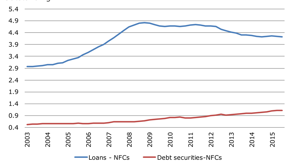
Note: The source is European Central Bank. All variables are in Euros trillions.
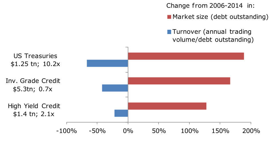
Note: The sources are SIFMA, FINRA TRACE and Goldman Sachs Global Investment Research.
2.3 Evidence from some key regulatory studies
We now turn to the empirical studies of market liquidity published by several prominent regulatory organisations or their employees. The most widely cited contributions are by researchers at the Federal Reserve Bank of New York (FRBNY).[18] They summarize their findings as follows:
“In conclusion, the price-based liquidity measures—bid-ask spreads and price impact— are very low by historical standards, indicating ample liquidity in corporate bond markets. This is a remarkable finding, given that dealer ownership of corporate bonds has declined markedly as dealers have shifted from a “principal” to an “agency” model of trading. These findings suggest a shift in market structure, in which liquidity provision is not exclusively provided by dealers but also by other market participants, including hedge funds and high-frequency-trading firms.”
They arrive at this conclusion by looking at a variety of standard measures of market liquidity. First, they document the decline in broker/dealer inventories by using the reports of primary dealers routinely reporting to the New York Fed (see Figure 2.3.1).[19] This decline has coincided with a period of very strong growth of both the investment grade and high yield segments of the US corporate bond market as depicted in Figure 2.3.2. They document a slight uptrend in trading volume (as seen in 2.3.3). (Note that they do not express turnover as a fraction of total market size. Had they done so, they would have shown a decline in trading volume.) They show that trade frequency has increased while trade sizes have declined (see 2.3.4). On this basis, they conclude
16 They comment, however, on the fact that corporate bond bid-ask spreads are wider than before the crisis.
that the market is adapting its trading style to mitigate the effects of declines in (i) dealer inventories and (ii) principal based liquidity provision.
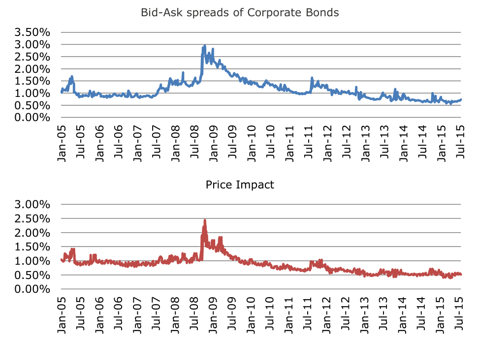
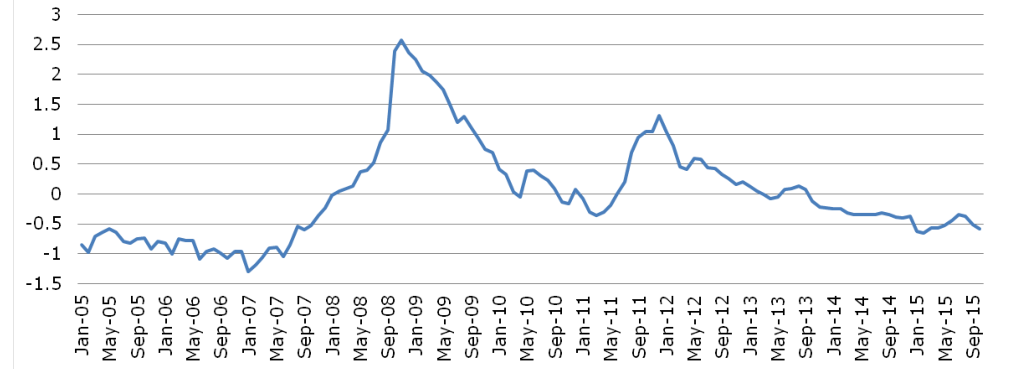
The remaining arguments of the FRBNY analysts’ draw on price-based measures of liquidity as depicted in Figure 2.4. The upper panel of 2.4 shows the effective spread equalling the difference between the dealer to client buy price and the dealer to client sell price averaged across all bonds. The chart shows a decline in the spread after the crisis and that the 2015 level lies below that in 2006.
Note that this averaging places greatest weight on the bonds that trade most frequently. Thus, if there has been a shift away from trading certain bonds that are traditionally illiquid toward large benchmark issues, this could give rise to the decline in the chart even though the effective spreads for benchmark issues and traditionally illiquid bonds may both be higher in 2015 than in 2006.
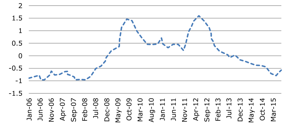
Finally, they report (see the lower panel in Figure 2.4) a price impact measure based on their version of the well-known Amihud ratio (discussed below). Again, they average across all traded bonds. The comment just made about their spread measure applies equally here. The decline could be attributed to a shift of trading away from categories of bonds that are relatively illiquid toward bonds that are traditionally liquid, i.e., by the increased bifurcation of the market.
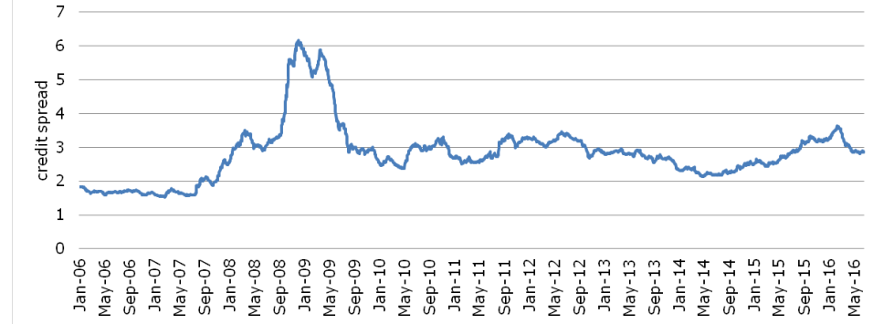
It is worth noting that the dominant features of the reported price based indicators of market illiquidity shown in Figure 2.4 are their extraordinary rise during the crisis in late 2008 and subsequent sharp fall. These are common features for a whole wide range of market indicators suggesting the presence of a single common risk factor in the financial system. For example, this is a main feature of the credit spreads as indicated in the follow chart of an index of Baa corporate yields versus 10 year US treasuries as depicted in Figure 2.5.
At about the same time as the FRBNY study, European regulators responded to widespread concerns about market liquidity with their own studies of corporate bonds in their own national markets.
A study of the French market undertaken by the French markets regulator, the Autorité des Marchés Financiers (AMF), was issued in late 2015 (see AMF (2015)).[20] The main conclusions of the study are that
1. After the two stress episodes in 2007-2009 and 2011, liquidity has improved steadily in French bond markets, beginning in early of 2012 but still suggests liquidity is lower than before the crisis in the 2005-2007 period.
2. Liquidity has become more concentrated in less risky instruments or in those that offer the greatest market depth.
3. There is evidence that changes in liquidity are essentially due to factors of a cyclical nature (especially what AMF (2015) describes as “risk aversion” but which might also be called perceived risk). Table 2.1 shows the AMF’s findings on overall turnover and other measures of market activity since 2010. Note that trading volumes increased between 2010 and 2014 as did average trade size. This is in contrast to the findings of the FRBNY study. This observation lies behind the AMF’s conclusion that activity has gravitated to the largest, most liquid issues. On average in the AMF sample, bonds trade about three times per day. This frequency is higher than that found by most corporate bond studies and may reflect the relative importance of benchmark issues in their sample.
An important focus of the AMF study is the behaviour over time of a composite indicator of market liquidity. The indicator is an equally weighted average of measure of bid/ask spreads, zero-returns (suggesting stale prices), and a measure of price impact. The three component measures are all expressed as normalised deviations from a within-sample mean. The AMF’s spread measure is based on an average of the
Bloomberg daily bid/ask spread in price terms divided by the residual maturity of the bond. Note this approach places particular weight on shorter-term issues. The zero return measure is the proportion of bond for which the best buy and sell prices were unchanged over the day. Price impact is measured by the ratio of the standard deviation of intraday returns to the square root of the sum of trading volumes.[21]
Figure 2.6 displays the composite illiquidity measure which is the main focus of the AMF paper. It shows the sharp increase in illiquidity as the crisis peaks first in 2008 and then a progressive fall. This time path closely resembles that of the price measures of market illiquidity in the NY Fed study. In contrast with the latter study, the AMF indicator exhibits a second smaller bout of market illiquidity in late 2011 and early 2012, reflecting the euro zone sovereign debt crisis.
The AMF report includes some additional evidence of a less aggregate nature which sheds light on differences in liquidity across different types of instruments. Table 2.2 (based on Table 2 in their study) reports measures of activity for government agency bonds, financials and non-financial corporations separately. It shows much higher turnover for government agency issues than for corporates and relatively high numbers of trades in non-financial corporates (compared to financials) in 2010 (about
4 trades per day). Turnover ratios (as a proportion of amount outstanding) are fairly constant throughout.
Finally, AMF (2015) reports the composite illiquidity indicator for the three bond market segments they consider. According to the composite measure, the corporate segment is significantly less liquid than the government segment. While we find this interesting, it still does not reveal much of a structural nature because these indicators remain extremely aggregative and are dominated by the influence of a single cyclical driving factor.
The AMF also present a composite indicator of “risk aversion” based on credit spreads, long and short rate slopes, the France-Germany government bond spread and the interbank spread. See Figure 2.7. They show that this is highly correlated with their composite liquidity indicator. Again, one may deduce the presence of a single common risk factor represent prevailing levels of market risk. This masks the possible influence of other dimensions of market liquidity either structural or themselves cyclical in nature.
The AMF study of market liquidity was followed by an analysis of corporate bond liquidity in the UK undertaken by Aquilina and Suntheim, researchers in the Financial Conduct Authority (FCA).[22] Similar to the AMF analysis, their study employs regulatory filings mandated under MiFID 1. The data they employ runs from 2007 to 2014 but the authors express doubts about the quality of reporting in the early years of the dataset. They present a variety of liquidity indicators. These include averages across bonds and days in each quarter Amihud price impact measures, minus the autocovariance of transaction returns (i.e., a Roll type measure), an Imputed Roundtrip Cost (IRTC), and volatilities in the Amihud and IRTC measures. They also calculate quarterly averages across bonds of average turnover rates and the fraction of days in each quarter on which bonds do not trade. Finally, they present information on dealer inventories drawn from regulatory filings.
The main findings of the Aquilina and Suntheim study are in line with those of both the New York Fed and the French regulatory study:
1. Inventories have declined while liquidity has recovered since the crisis.
2. Liquidity risk as measured by the volatilities of their price-based liquidity indicators has also fallen back since the crisis.
3. The liquidity component of yield spreads is declining or stable.
4. Liquidity could still decline under stress.
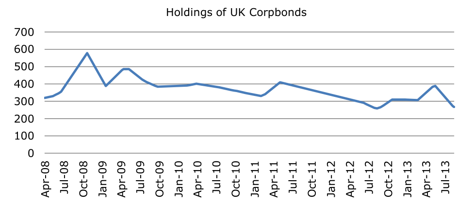
These conclusions are supported by the following evidence. Figure 2.8 suggests a declining trend in dealer inventories.
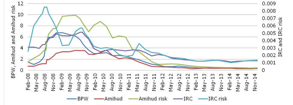
Figure 2.9 exhibits individual price based measures calculated by Aquilina and Suntheim. Here “BPW” is the measure equal to minus one times auto-covariance of returns suggested by Bao, Pan, and Wang (2011) (which closely resembles a measure introduced by Richard Roll). “Amihud risk” and “IRC risk” denote the standard deviations within each quarter of the daily indicators.
While there are some detailed differences in the behaviour of these measures, the dominant message of the chart which also serves as the basis of the report’s main conclusion is that illiquidity rose sharply during the crisis but declined subsequently to extremely low levels by end 2014.
The FCA researchers also examine trends in turnover and zero turnover. The fraction of bonds that did not trade on a given day averaged over the quarter were slightly higher early in the sample period. The typical corporate bond traded once in five days. Zero trading days were less on average in the second half of the sample period, but this appears to reflect the development by the FCA of a different reporting system. Turnover appears to be higher in the latter half of the sample, again possibly reflecting the change in reporting systems or a changing composition of trades with more trading in larger, benchmark issues as suggested by AMF (2015).
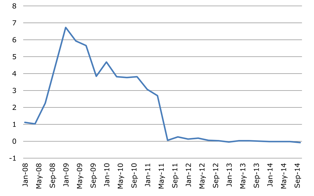
Aquilina and Suntheim combine the various measures of market illiquidity in a composite measure. As one might expect, when calculated for the whole sample, this measure captures the peak illiquidity during the crisis followed by a subsequent steep decline. This is seen in Figure 2.10.
The authors also report cross-sectional differences in the composite illiquidity measure based on age of issue, residual maturity of issue and credit quality. The results are reported in Table 2.3. The most important regularity is that illiquidity is increasing in the age of the issue with a significant regular decline in liquidity within the first two years of issuance.
One might infer from this that corporate bonds trade actively after issuance until they progressively gravitate to portfolios of long-term investors who trade infrequently. Differences in maturity do not seem clear drivers of liquidity, although perpetuals appear to be relatively illiquid. Finally, Aquilina and Suntheim find that liquidity appears to increase with credit quality.
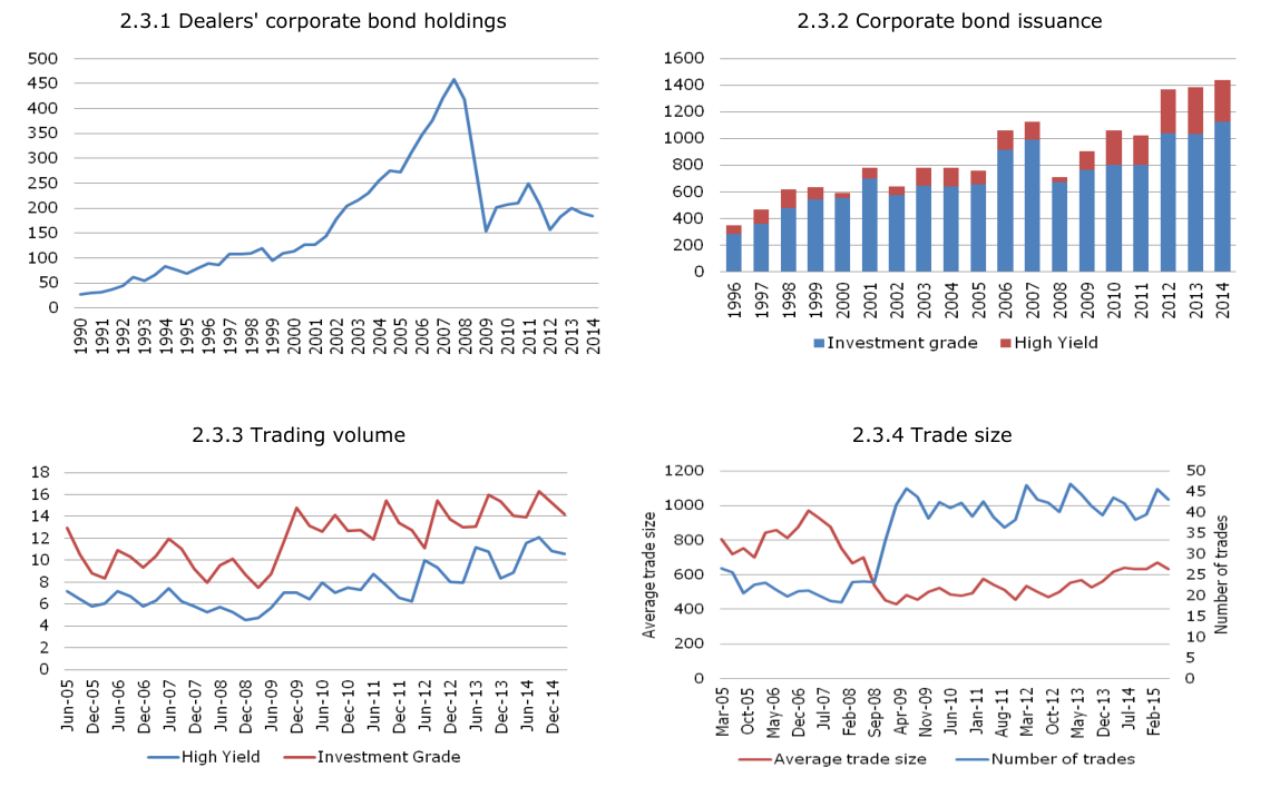
Note: All variables are in USD billions except Trade size in Figure 2.3.4. Average trade size is in USD thousands and Number of trades is in thousands. The source for dealers’ corporate bond holdings is Federal Reserve Board. The source for corporate bond issuance is SIFMA. The source for Trading volume and Trade size is TRACE. Dealers’ corporate bond holdings shows the quantity of corporate and foreign bonds (held in US) owned by securities brokers and dealers. Corporate bond issuance shows annual issuance of IG and HY corporate debt. Trading volume shows average daily trading volume by quarter for IG and HY corporate debt.
Note: The source is the Federal Reserve Bank of St. Louis. The variable is in percent.
Note: Sources are AMF and Bloomberg.
Note: The sources are AMF and Bloomberg.
Note: The source is FCA. Variables are in GBP billions.
Note: The source is Aquilina and Suntheim (2016). Lower values imply a more liquid market. Indicators are quarterly averages.
| Outstanding | Outstanding | Number | Trading | Number of | Average | Number of | Monthly | |
|---|---|---|---|---|---|---|---|---|
| amount, | amount, | of bonds | volumes | trades | trade size | trades per | turnover | |
| Year | ||||||||
| French issuers | traded bonds | traded | (€ billion) | (thousands) | (€ million) | bond | ratio | |
| (€ billion) | (€ billion) | |||||||
| 2010 | 3,092 | 2,553 | 2,325 | 4,395 | 1,848 | 2.4 | 795 | 14% |
| 2011 | 3,368 | 2,688 | 2,547 | 5,290 | 1,972 | 2.7 | 774 | 16% |
| 2012 | 3,424 | 2,836 | 2,517 | 5,022 | 2,109 | 2.4 | 838 | 15% |
| 2013 | 3,452 | 2,891 | 2,432 | 5,270 | 1,985 | 2.7 | 816 | 15% |
| 2014 | 3,585 | 2,936 | 2,435 | 5,567 | 1,761 | 3.2 | 723 | 16% |
| 2015 | 3,717 | 2,803 | 2,163 | 3,737 | 1,329 | 2.8 | 614 | 15% |
Note: The source is the AMF. The second column shows outstanding year-end amounts of bonds of French issuers taken from BIS statistics and converted to EUR. The data for 2015 go to end- March. The third column shows an estimated annual outstanding amount equal to the sum of issued amounts for bonds in which a trade was reported. Note that this approach underestimates the outstanding amount of topped-up issues. In all cases, the data for 2015 go to the end of September.
| Year | Supra-Gov-Agencies | Bank-Financial | Non-Financial |
|---|---|---|---|
| Number of Monthly | Number of Monthly | Number of | |
| trades per turnover | trades per turnover | trades per | |
| bond ratio | bond ratio | bond ratio | |
| 2010 | 1627 18% | 426 7% | 1273 8% |
| 2011 | 1746 21% | 407 8% | 1229 9% |
| 2012 | 1496 19% | 484 7% | 1340 7% |
| 2013 | 1325 20% | 538 6% | 1124 7% |
| 2014 | 1271 21% | 482 7% | 905 7% |
| 2015 | 1056 19% | 456 7% | 653 8% |
Note: The source is the AMF. The data for 2015 go to the end of September.
| Composite | ||
|---|---|---|
| measure | ||
| <3m | -0.06 | |
| 3m to 1y | -0.035 | |
| Age | ||
| 1y to 2y | -0.01 | |
| >2y | 0.16 | |
| 0-2y | 0.05 | |
| 2-5y | -0.05 | |
| Maturity | ||
| >5y | 0.02 | |
| Perpetual | 1.33 | |
| AAA | -0.12 | |
| AA | -0.07 | |
| Rating | A | -0.01 |
| BBB | 0.03 | |
| Speculative | 0.29 |
Note: The source is Aquilina and Suntheim (2016) calculations. Lower values indicate higher liquidity.
2.4 More recent regulatory studies
The studies of the FRBNY, the AMF and by Aquilina and Suntheim that we have just reviewed are not the only studies by regulators in this area[23], but they have been very influential in forming a consensus in the regulatory community on the issue of whether there is a fundamental problem of secondary market illiquidity that requires action by public authorities.
Recently, IOSCO (2017) has issued the final report of the review of secondary market liquidity in corporate bonds world-wide. It is based on a review of regulatory and academic studies as well as a survey questionnaire made of selected national regulators. Its conclusions are largely in line with those of the three regulatory studies discussed above. Specifically, it states:
“Based upon its detailed analysis of liquidity metrics, survey results (both qualitative and quantitative) from industry and regulators, roundtables with industry, and a review of academic, government and other research articles, IOSCO did not find substantial evidence showing liquidity has deteriorated markedly from historic norms for non-crisis periods. IOSCO also notes that there is no reliable evidence that regulatory reforms have caused a substantial decline in the liquidity of the market, although regulators continue to monitor closely the impact of regulatory reforms.”
This conclusion was based mainly on metrics supporting improved liquidity, namely, price impact and bid-ask spreads. However, they acknowledge that evidence was mixed on trade sizes and turnover. Furthermore, there was some evidence that block sizes have become smaller (which they suggest might reflect more electronic trading) and signs of a decline in dealer inventories as large players retreat from the principal model of market making.
Other regulatory studies that have been completed since the initial FRBNY, AMF and Aquilina and Suntheim analyses suggest important qualifications to the conclusions of the early studies. A recent study by analysts at ESMA (De Renzis et al. (2016)), reconsiders the evidence based on publicly available information since 2014. While their overall conclusion is that the evidence falls short of showing a strong, widespread decline in activity, they note that bid-ask spreads point to lower liquidity as average spreads increased by 12 basis points between the beginning of 2015 and 2016.
Furthermore, ESMA (2016) use a merged Markit-Euroclear dataset in Euro denominated corporate bonds and find that the average monthly number of settlements per bond declined in the period analysed across different rating categories. This means that while it would have taken 55 days to close a $50 million position in March 2015, by March 2016 it would have taken 70 days.
FRBNY researchers have also added a qualification to their earlier study (see Adrian et al. (2016)). In response to comments they received criticising their use of broad averages of liquidity measures, they provided further analysis examining how corporate bond market liquidity has changed over time depending on the size and credit rating of the issue.
In effect, they carried out a limited conditional analysis of the type we have argued above is required before we have a clearer assessment of possible structural changes. They obtain mixed results. They find that trade sizes have declined compared to precrisis levels for bonds of all issue sizes. Bid-ask spreads are decreasing with issue size but for any given size, recent spreads are comparable to pre-crisis levels. Finally, for any given size category, their measure of price impact is lower in recent periods than before the crisis.
A more significant qualification to previous analysis is made by FCA (2017) which makes the following overall assessment:
“New data suggests there has been a decline in liquidity in the UK’s corporate bond market over the past two years. The analysis, which combines both traditional and non-traditional measures of liquidity, indicates trading conditions have generally become more difficult from 2014/2015 onward.”
The “traditional measures of liquidity” to which they refer are those shown in Figure 2.9. These indicate a decline in liquidity in the 2015-2016 period. To assess the practitioner argument that it is more difficult to source liquidity, to execute a trade and to make a significant change of position, FCA (2017) present data obtained from corporate bond trading platforms. They find that there has been an increase in the number of times Requests for Quotes[24] fail to result in a trade. Furthermore, there has been a notable increase in the proportion of bonds that simply do not trade in a given week.
We close this section by reviewing one additional study based on regulatory data that was undertaken by a working group of the European Systemic Risk Board (ESRB) made up of official sector analysts from a number of EU member states.[25] The focus of this study was shadow banking, understood broadly as non-bank credit creation, and its contribution to systemic risk in Europe. However, the study also touched upon the market liquidity of European corporate bond markets.
As has been argued previously, an important contributing factor in the provision of liquidity by market makers is the ease with which they can take a position in a single name security should they wish to do so. One factor that contributes to this is securities lending. On this point, the ESRB study documents a substantial decline in the securities lending of EU corporate bonds that has taken place since the crisis.
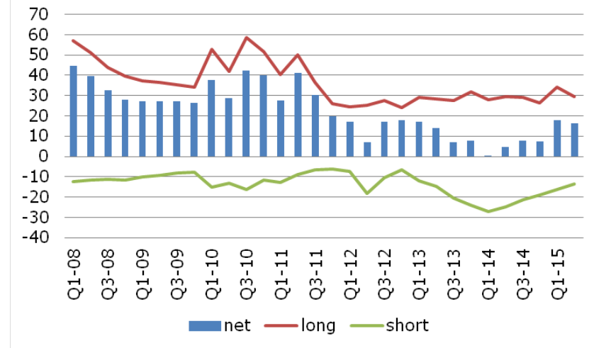
The study also reports information on market maker inventories not based on aggregate measures of the net assets in overall group balance sheets but rather coming from a survey of selected large market-makers in which they report the evolution of the dedicated market maker inventories. The results point to a dramatic drop in dealers’ inventories since 2013 Q1. This is depicted in Figure 2.11. We shall use this inventory data in some of our econometric analysis in Section 8 below.
Note: The source is Grillet-Aubert et al. (2016). Data shows investment grade non-financial inventory data collected from 13 EU market-makers. Units are EUR billions.
3. Drivers of Liquidity
Summary of findings:
1. We construct several substantial datasets that permit us to examine trading activity and price-based measures of liquidity across the entire EU market. Bonds that appear at least once in our datasets were issued in 27 countries, comprise 28,902 individual bonds and have a par value of EUR 8.2 trillion. Those present at 1st July 2016 amounted to 16,741 bonds with a par value of EUR 4.3 trillion.
2. The market size has expanded in recent years but activity indicators such as numbers of transactions, fractions of bonds traded and turnover rates have declined, particularly for non-financial bonds.
3. Activity indicators extracted from recent clearing data suggest generally similar trends.
4. Trading cost indicators including bid-ask spreads, effective spreads recorded on an Electronic Trading Platform (ETP) and round-trip measures fell after the crisis but have recently shown a noticeable upward tendency.
5. Market depth indicators such as Amihud ratios again fell after the crisis but since 2014 have risen, in some cases markedly.
6. When bid-ask spreads and ETP effective spreads are calculated for sets of bonds holding return volatility constant, it appears that trading costs rose substantially in the crisis and never fell back.
7. Having examined trends for liquidity indicators both in aggregate and broken down by category, we use panel data regression analysis to study how the indicators behave holding cross-sectional and time series drivers like risk (measured using ISIN-level and aggregate return volatilities) constant. We find that, holding these influences constant, time trends are significant and negative for turnover and trade numbers, and positive for ticket size and for the fraction of bonds not traded.
8. Again, holding other drivers constant (by performing regressions), we find that the price-based indicators show varying time trends. Such linear trends are difficult to interpret as the price-based indicators generally exhibit u-shaped time paths over the sample period of the FCA data (which starts after the crisis has begun).
3.1 Introduction
This section presents analysis of the determinants of liquidity in European corporate bond markets. To understand if structural changes have occurred in corporate bond market liquidity since the crisis, one must go beyond past studies. This requires detailed identification of liquidity drivers and comprehensive analysis of bond markets across the European Union.
We focus on market liquidity at the level of individual securities and study liquidity in multiple dimensions. The dimensions include
a) Transaction volumes
b) Turnover ratios
c) Numbers of trades
d) Ticket size
e) Bid-offer spreads based on quote data
f) Effective spreads
g) Round trip costs
h) Measures of price impact including Amihud ratios and BPW/Roll statistics.
Determinants of market liquidity that we examine include
a) Issue characteristics (such as size, age issue, credit quality and past volatility)
b) Issuer characteristics (such as country and sector of activity)
c) Risk indicators (both individual and market average return volatilities)
Key to understanding market liquidity, especially in bond markets, is differentiating the influence of liquidity from that of risk. In periods of credit market stress, bond prices typically fall well below par values as credit spreads widen. In such circumstances, dealers charge more to provide immediacy so transactions-cost related measures of liquidity rise. This occurs whether or not markets are functioning well in the sense of efficiently intermediating between bond buyers and sellers.
Many past studies of liquidity focus on changes in liquidity indicators (such as trading costs and market depth measures) that are closely correlated with changes in the riskiness of the securities involved. Among other objectives, this section aims to examine liquidity conditional on risk as measured by lagged volatility.
The remainder of this section is organised as follows. Section 3.2 describes data sources and coverage. Section 3.3 discuss activity-based indicators of liquidity that reveal trends in the levels of trading. Section 3.4 looks at price-based liquidity measures which capture the costs of secondary market trading.
3.2 Data
The datasets that we employ in our empirical analysis may be described as follows.
1. Regulatory MiFID 1 data provided by the UK’s Financial Conduct Authority. Under the Markets in Financial Instruments Directive (commonly referred to as “MiFID 1”), regulated firms are required to report transactions via an Approved Reporting Mechanism. Such mechanisms provide validation after which the reports are transmitted to national regulatory bodies such as the FCA.[26] The reports provide extensive information on the time, size, venue, and counter-parties involved in individual trades and security identifiers such as the ISIN of the security in question.
To facilitate this study, the FCA provided us with access to the MiFID 1 data for corporate bonds. The central role within European bond trading of the City of London means that the FCA’s MiFID 1 data covers much of the European market. Thus, for example, the data includes a comparable number of transactions for French as for UK bonds. The MiFID 1 data employed in this study covers transactions from September 2011 to August 2016 with an average number of daily transactions equalling 9,190 and an average daily volume of €5.4 billion.
2. Bond settlement data provided by the major European post-trade services organisation Euroclear. Euroclear holds accounts valued at €27.5 trillion of securities on behalf of more than 2,000 clients including major custodian banks. The securities covered reportedly include more than 60% of the Eurobond market.[27]
Note that the Euroclear data provides information on settlements not transactions between beneficial owners. Hence, transactions between counterparties that are both registered with a single member of Euroclear will not typically show up in the data.
Euroclear provides settlement services through several legal entities. We obtained data from three of these: Euroclear Bank, Euroclear Settlement of Euronext-zone Securities (ESES) and Euroclear UK & Ireland. Of these, the most substantial data comes from ESES and comprises data on 1,014,019 corporate bond transactions in the period January 2014 to August 2016.
3. Data on European corporate bond transactions from one of the major electronic trading platforms on which institutional clients request quotes (RFQs) from dealers. This data permits one to calculate effective spreads on a large number of European corporate bond transactions between February 2010 and November 2016. The number of corporate bond ISINs included in the platform was 4,125 at the end of the sample period.
4. Bond quote data from Bloomberg. These include daily quotes (bid and ask) since 1990 for 9,403 European corporate bonds. The bonds include issues from all the current EU28, whether or not they were members of the EU at the time.
5. Bond and issuer characteristic data from the Eikon database supplied by Thomson Reuters. These include currency, coupon, issuer domicile and issuer sector.
More information on data sources is provided in Annex 1.
The combination of these data sources constitutes a comprehensive dataset on European corporate bond trading. The FCA data covers trading in 21,542 bonds from
2011. The Euroclear data provides settlement information on 4,567 bonds. The ETP data includes detailed transaction and quote data for 7,053 different electronically traded bonds. The daily quote data from Bloomberg goes back to 1990 and, by 2016, covers 9,403 distinct corporate bonds.
How does the coverage of this analysis compare to past studies? The most comprehensive previous study of European corporate bond liquidity covering the precrisis period was that of Biais et al. (2006). This employed data on about 1,400 bonds between 2003 and 2005. The recent French regulatory study of the corporate bond market (AMF (2016)) examines the period 2005-2015 and includes 2,900 corporate bonds (most being financial issues) for which the AMF is the responsible supervisor. Finally, Aquilina and Suntheim (2016) analyses the 6,291 corporate bonds (most financial) for which the FCA is the supervisory authority. The period covered is 2007-
2014 but much of the analysis focuses on post 2011 when the Zen[28] data became available.
Detail of the coverage and overlap of the datasets we employ are provided by Tables 3.1-3.4. Table 3.1 shows the number of bond ISINs in the datasets broken down by 27 European Union countries. All countries have some representation but clearly most ISINs come from the major bond issuing countries: UK, Netherlands, France, Germany, Italy and Luxembourg.
The FCA dataset contains more than double the ISINs of the other datasets when all the sample periods are considered. The Bloomberg data contains about double the number of ISINs in the Euroclear dataset and somewhat more than the number in the Electronic Trading Platform (ETP) transactions dataset.
Some aspects of the distribution across countries are of interest. For example, the Euroclear dataset contains almost as many French bond ISINs as does the FCA data. For some other countries, like the UK and Germany, the FCA data has a large multiple of the ISINs present in other datasets. Table 3.2 shows the same data but for the ISINs present in the dataset at the end of the sample period. The patterns apparent from the table are broadly similar to those of Table 3.1.
Tables 3.3 and 3.4 show the breakdown of the different datasets based on the par value of the bonds covered. As with the earlier tables, the first table shows results for all bonds appearing in the datasets at any time, whereas the second table presents results for the bonds present in the dataset in the final month of the sample period.
It is interesting that the total par values of the FCA, Bloomberg and ETP datasets are comparable, being about €5 trillion when all bonds ever appearing are considered (see Table 3.3). When only bonds present in the final period are considered, the Bloomberg dataset is slightly larger than the others with €3.4 trillion of par value.
On the basis of these comparisons, one may conclude the dataset examined here constitutes the most comprehensive yet constructed for analysing European corporate bonds’ liquidity.
| Netherlands | Luxembourg | |||||||||||||
|---|---|---|---|---|---|---|---|---|---|---|---|---|---|---|
| Austria | Spain | Germany | France | Ireland | Sweden | Finland | Belgium | Denmark | Slovenia | |||||
| Italy | UK | |||||||||||||
| Bloomberg | 589 | 242 | 2,128 | 303 | 544 | 1,561 | 1,756 | 443 | 220 | 975 | 151 | 149 | 164 | 6 |
| Euroclear | 99 | 20 | 1,104 | 77 | 115 | 2,230 | 481 | 116 | 30 | 110 | 47 | 100 | 29 | 1 |
| FCA | 1,000 | 444 | 7,250 | 562 | 1,671 | 2,714 | 4,771 | 1,195 | 594 | 523 | 169 | 195 | 221 | 15 |
| ETP | 643 | 91 | 1,554 | 357 | 495 | 1,467 | 1,307 | 280 | 208 | 265 | 85 | 110 | 113 | 1 |
| Rep | ||||||||||||||
| Estonia | Greece | Hungary | Portugal | Bulgaria | Cyprus | Croatia | Czech | Romania | Slovakia | Latvia | Malta | Poland | Total | |
| Bloomberg | 5 | 7 | 8 | 75 | 3 | 22 | 14 | 21 | 5 | 3 | 3 | 6 | 0 | 9,403 |
| Euroclear | 2 | 2 | 1 | 18 | 1 | 10 | 1 | 1 | 1 | 2 | 0 | 0 | 0 | 4,598 |
| FCA | 2 | 4 | 7 | 139 | 5 | 23 | 3 | 23 | 6 | 4 | 0 | 1 | 1 | 21,542 |
| ETP | 1 | 3 | 6 | 56 | 0 | 2 | 1 | 8 | 0 | 0 | 0 | 0 | 0 | 7,053 |
Note: Country indicates the location of the registered office of the issuer. This is the approach to company location used by Thomson Reuters. Bonds issued by the foreign subsidiary of a company, therefore, are assigned to the country in which the subsidiary has its registered office.
| Netherlands | Luxembourg | |||||||||||||
|---|---|---|---|---|---|---|---|---|---|---|---|---|---|---|
| Austria | Spain | Germany | France | Ireland | Sweden | Finland | Belgium | Denmark | Slovenia | |||||
| Italy | UK | |||||||||||||
| Bloomberg | 448 | 175 | 1,554 | 197 | 355 | 1,133 | 1,204 | 297 | 143 | 858 | 123 | 123 | 119 | 4 |
| Euroclear | 75 | 13 | 884 | 51 | 86 | 1,587 | 319 | 96 | 21 | 91 | 32 | 79 | 23 | 1 |
| FCA | 511 | 264 | 4,136 | 274 | 782 | 1,652 | 2,792 | 646 | 356 | 353 | 102 | 132 | 104 | 6 |
| ETP | 343 | 52 | 991 | 179 | 300 | 803 | 720 | 182 | 108 | 152 | 49 | 80 | 56 | 1 |
| Rep | ||||||||||||||
| Estonia | Greece | Hungary | Portugal | Bulgaria | Cyprus | Croatia | Czech | Romania | Slovakia | Latvia | Malta | Poland | Total | |
| Bloomberg | 4 | 0 | 5 | 53 | 2 | 12 | 11 | 16 | 2 | 3 | 2 | 1 | 0 | 6,844 |
| Euroclear | 2 | 0 | 0 | 16 | 1 | 8 | 1 | 1 | 1 | 0 | 0 | 0 | 0 | 3,388 |
| FCA | 2 | 2 | 3 | 88 | 2 | 10 | 3 | 16 | 2 | 4 | 0 | 1 | 1 | 12,244 |
| ETP | 1 | 1 | 2 | 29 | 0 | 1 | 1 | 3 | 0 | 0 | 0 | 0 | 0 | 4,054 |
| Number | ||||||
|---|---|---|---|---|---|---|
| of | ISINs | Par | ||||
| as | of | value as | ||||
| Number | total | Par Value | of | total | ||
| of ISINs | (%) (€ | billion) | (%) | |||
| Bloomberg | 9,403 | 32.53 | 4919.53 | 59.64 | ||
| Euroclear | 4,598 | 15.91 | 1529.01 | 18.54 | ||
| FCA | 21,542 | 74.53 | 5423.18 | 65.75 | ||
| ETP | 7,053 | 24.40 | 4870.02 | 59.04 | ||
| Combination | ||||||
| of all the | 28,902 | 100 | 8248.69 | 100 | ||
| datasets |
| of | ISINs | Par | ||||
|---|---|---|---|---|---|---|
| as | of | value as | ||||
| Number | total | Par Value | of | total | ||
| of ISINs | (%) | (€ billion) | (%) | |||
| Bloomberg | 6,844 | 40.83 | 3,399.28 | 78.91 | ||
| Euroclear | 3,388 | 20.21 | 1,062.89 | 24.68 | ||
| FCA | 12,244 | 73.05 | 2,885.50 | 66.99 | ||
| ETP | 4,054 | 24.19 | 2,607.59 | 60.54 | ||
| Combination | ||||||
| of all the | 16,761 | 100 | 4,307.53 | 100 | ||
| datasets |
3.3 Activity-based indicators of European corporate bond liquidity
3.3.1 Distinguishing price- and activity-based indicators
To understand the behaviour of market liquidity for European corporate bonds, one may use the data just described to create liquidity indicators and then analyse their behaviour over time. We perform the analysis unconditionally, studying the paths the indicators follow, and conditionally. The conditional analysis consists of studying liquidity indicators for particular subsets of bonds and performing regression analysis.
We distinguish between “price-based” and “activity-based” indicators of liquidity. Activity-based indicators include volume, turnover ratios, ticket size, and number of trades. These measures are common in past studies of bond market liquidity. In addition, we look at such measures as the fraction of business days in the month on which there is at least one transaction and the fraction of days with a month on which the bond does not trade at all.[29] Price-based indicators include bid-ask spreads, effective spreads, round trip costs, and market depth measures. These will be examined further below. As a systematic approach, we form monthly averages over individual ISINs of particular liquidity indicators.
We investigate the activity-based measures using three data sources: the FCA, Euroclear and ETP datasets. Each provides a distinct perspective. The FCA dataset is particularly comprehensive in that it covers a wide range of corporate bond transactions from different venues including bilaterally negotiated trades involving large dealers and also on the proprietary platforms operated by single dealers. The Euroclear dataset covers a wide range of corporate bonds at the settlement level (revealing movements between custodian accounts). The ETP data gives insights into the characteristics of bonds amenable to electronic trading.[30]
3.3.2 Activity-based indicators from regulatory data (FCA)
The FCA data are very valuable for our study because of their detailed nature and the broad cross-sectional coverage they provide of the corporate bond market. Furthermore, since they cover the period between 2011 and 2016, they extend over a reasonably long period that includes the introduction of some major regulatory changes and the sovereign debt crisis in Europe.
Figure 3.1 provides information about the corporate bonds covered by the FCA transactions data. The total amount outstanding of these bonds rises from €2.9 trillion in 2011 to €3.2 trillion in 2016. This rise reflects the strong rate of primary issuance as European corporates have used the opportunity of low rates to seek funding while relying less on bank loans than has historically been the case. The higher level of new issuance has boosted the size of the secondary market and, ceteris paribus, tended to increase aggregate turnover volumes.
Of the total value outstanding in 2016, UK and French corporate bonds account for about €0.8 trillion each while Netherlands bonds contribute €0.6 trillion. Both Italian and German corporate bonds represented €0.2 trillion in 2016. (More detailed data for these and other countries can be found in Annex 1.) While the total amount outstanding rose by about 10% between 2011 and 2016, the amounts outstanding of German and Italian bonds actually fell. The category that grew most is French bonds.
The large majority of the outstanding value of bonds covered by the FCA dataset traded is Euro denominated. About a quarter of the outstanding value of bonds traded in 2016 consists of non-financials (€0.8 trillion compared to €2.4 trillion for financials).
Figure 3.2a presents a set of activity indicators for the category of all bonds in the FCA dataset. The indicators consist, in all cases, of monthy averages across individual ISINs. To be specific, the upper left figure (3.2a.1) consists of the average ticket size for all transactions in a given month. The upper righthand figure (3.2a.2) shows the average across ISINs of the ratio of the monthly turnover (expressed on a daily basis) to the amount outstanding at the start of the month.
The lower lefthand figure (3.2a.3) shows the fraction of bonds traded at least once during the month in question. The lower righthand figure (3.2a.4) shows the mean number of daily transactions across ISINs within the month in question.
The figures show some striking trends over the 2011-16 period. Mean ticket sizes have risen by about 20% over the period from around €0.5 million to €0.6 million. This seems to contradict the argument advanced in some practitioner studies that reduced liquidity has obliged investors to work orders more by engaging in smaller trades.
Mean daily turnover rates for bonds trend down slightly starting in 2014. The fraction of days within a month on which individual ISINs trade shows a strong downward trend from 41% to 34% between 2011 and 2016. The mean number of transactions across ISINs has also declined substantially from approaching 1 to about 0.6.
Figure 3.2b shows activity trends (similar to those for corporate bonds as a whole in Figure 3.2a) for non-financial bonds. The trends resemble those for all bonds but are more marked. In particular, the decline in mean daily turnover in 3.2b.2 is much clearer with an approximate one third decrease over the sample period. The mean number of daily transactions is about halved (in contrast to the decline of about a third for corporate bonds as a whole).
The fraction of bonds traded at least once in a month (shown in 3.2b.3) is much higher as a level than the comparable fraction for corporate bonds as a whole (see 3.2a.3). In both cases, the decline is about a seventh of the fraction. Last, the mean tickets size shown in Figure 3.2b.1 is quite similar to those for corporate bonds as a whole both in levels and in the strong growth rate over the sample period.
To understand aggregate trends in activity, it is helpful to break down the results for the market as a whole into subcategories. The figures below show how the activity indicators behave for narrower categories of bond.
Figure 3.3 presents the average daily transaction volume (total transaction volume in the month/number of business days in the month) for individual bonds averaged across all bonds in a given category. The uppermost four plots show results for corporate bonds as a whole whereas the bottom two plots exhibit results for nonfinancial bonds only.
Figure 3.3.1 shows average monthly transaction volumes for bonds sorted by age. Young bonds (less than a year since issuance) trade in much larger volumes than older bonds. This reflects the life cycle of bond issues as securities are issued and initially traded but then gravitate to the portfolios of long-term investors where they tend to remain until maturity. This bond life cycle is important because as the size of the market has grown in recent years, one would expect turnover to higher reflecting the fact that young bonds are proportionally more numerous.
Figure 3.3.2 shows that non-financial bonds exhibit much larger average trading volumes than financial bonds. Figure 3.3.3 shows that large sized issues trade in larger volumes than do small issues (as one would expect). Finally, of the figures showing results for corporate bonds as a whole, 3.3.4 shows that Euro denominated issues tend to be traded in larger volumes than securities issued in other currencies.
The lower figures in 3.3 show results for non-financial bonds. The age effect is just as evident for non-financials. The issue size effect is much more graduated for nonfinancials than for bonds as a whole. While for the latter, the transactions volumes are radically higher for large bond issues, for non-financial bonds, there is less dominance by large issues although a monotonic increase in transactions volumes is evident for larger issues.
Figure 3.4 shows turnover rates. These are defined as the ratio of volume transacted in a given month in a given bond to the amount outstanding of that bond at the start of the month averaged over ISINs. The results resemble those for volume except that the decline in turnover rates for non-financials (see 3.4.2) is more clear cut and Euro and GBP denominated bonds exhibit comparable turnover rates.
Figure 3.5 shows mean transactions sizes, averaged across the ISINs in different categories. Figure 3.2a.1 already showed that ticket sizes have overall been rising since 2011. Figure 3.5.1 gives ticket sizes broken down by age. Ticket sizes tend to be larger for newly issued bonds. An upward trend is evident for each age category. Figure 3.5.3 shows that investment grade bonds tend to trade in much larger size than do High Yield bonds, while 3.5.4 shows that USD issues trade in larger lots than do EUR or GBP issues. All sub-categories of bond exhibit an upward trend in ticket size over time.
Figure 3.6 shows the mean number of transactions per day for different bond subcategories. Figure 3.6.1 shows that the mean number of transactions per day has remained reasonably high for new bonds but that trading frequency in seasoned bonds has fallen sharply. Again, this is an indication of bonds disappearing into hold-tomaturity silos. The age effect is evident also for non-financials alone (see 3.6.5) but in this case a downward trend appears present even in new bonds.
From 3.6.2, one may observe that non-financial bonds trade, on average, much more frequently, than financials, although the discrepancy has shrunk somewhat over time. Figure 3.6 also suggests that numbers of trades per day are higher for EUR and GBP issues than for USD issues (see 3.6.4). Both EUR and GBP issues exhibit downward trends in trade numbers. For non-financials, the mean number of trades for EURdenominated bonds has clearly trended down, whereas GBP-denominated bonds show flat transactions numbers. High yield bonds have more trades per day than investment grade (see 3.6.3).
Figure 3.7 shows (averaged over ISINs) the fraction of days in the month when there is at least one trade. This provides insight into characteristics of bonds that are barely traded at all. Figure 3.7.1 shows, as one would expect, that bonds that are close to maturity trade infrequently and that bonds with maturities over 5 years exhibit the largest fraction of trading days in the month.
The fraction of trading days in the month is non-monotonic in rating category in the sense that AAA and B or lower are the categories that are least traded by this measure (see 3.7.2). In other words, the most traded are bonds rated BB or BBB, i.e., the categories that bracket the dividing line between investment grade and high yield. One might hypothesise that such bonds exhibit increased trading frequency as investors are obliged by their mandates to dispose of bonds downgraded from BBB or may be able to buy bonds upgraded from BB. The distinction between ratings appears less noticeable when one focusses on non-financial bonds alone (see 3.7.6). Bonds closest to maturity trade least by this measure (see 3.7.4).
Figure 3.7.3 show that the fractions of trading days in the month is much higher for non-financials than financials and that both have declined for both non-financials and financials. Within the category of non-financials, Figure 3.7.5 shows that Italian and Germany bonds exhibit the highest fraction of trading days in the month whereas UK bonds are traded less by this measure.
Figure 3.8 shows the likelihood that bonds in different categories trade at least once in a given month. The plots provide insight into whether bonds in given categories tend to be siloed. As with Figure 3.7, there are some indications of information-driven trading (with ratings and maturity mattering). Figure 3.8.2 shows that bonds on either side of the IG/HY frontier tend to be more actively traded while AAA issues are quite unlikely to trade.
Non-financial issues are much more likely to trade than are financial issues (see 3.8.3). The likelihood that GBP denominated bonds trade has declined substantially whereas the fraction of bonds that trade at least once has remained flat for EURdenominated bonds (see 3.8.4).
The lower block of plots in Figure 3.8 show results for non-financial bonds alone. The country breakdown (see 3.8.5) shows a surprisingly high fraction of Italian bonds traded at least once a month.[31] There is less variation across rating categories than for bonds as a whole (see 3.8.6). A clear size effect is evident (3.8.7). The currency findings are altered somewhat in the case of non-financials in that the fractions of GBP and EUR-denominated bonds that trade at least once a month both appear to trend downward somewhat (see 3.8.8).
It is worth pausing to consider the broader themes that emerge from our exploration of the evidence on activity measures of liquidity in European corporate bonds. We think that four themes have been suggested by the FCA data:
1. Volume is driven by two conflicting factors—the number of bonds is growing but turnover rates in individual bonds are declining.
2. Young bonds have higher turnover and trade in large tickets. Older bonds trade less frequently and in smaller trades. These are clear indications of a bond lifecycle. Bonds begin in the hands of large dealers and are progressively distributed to long-term investors that tend to trade infrequently.
3. Information sensitive bonds trade more than do information insensitive bonds but irregularly depending upon the rate of information arrival.
4. Most bonds do not trade very frequently. As they age, their trading frequency declines.
We cannot claim that these tendancies are distinct causal factors or that other possible drivers of activity may not be part of the explanation of the apparent decline in rates of turnover at the individual bond level noted in our discussion of Figure 3.1. However, we think that the factors highlighted in these themes make sense. So it is natural to ask whether taken together they make for a reasonable explanation for the evolution of liquidity in the corporate bond market since 2011. Alternatively, are there additional drivers of liquidity, so far omitted from our analysis, that have depressed liquidity in recent years? This would be evidence that could be more supportive than previous regulatory tests of the hypothesis that liquidity provision is being challenged by regulatory and other structural changes. We will explore these issues below using more sophisticated multivariate techniques that allow one to examine the effects of multiple drivers simultaneously.
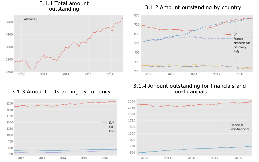
Note: All variables are in EUR billions. The total value outstanding for European corporate bonds has seen an increase over the sample period. This increase is most noticeable for French bonds and non-financials.
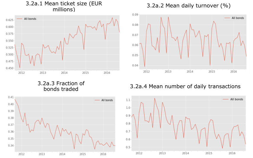
Note: Mean ticket sizes of European corporate bonds have risen steadily over the sample period, while the number of bonds traded and the mean number of daily transactions have declined.
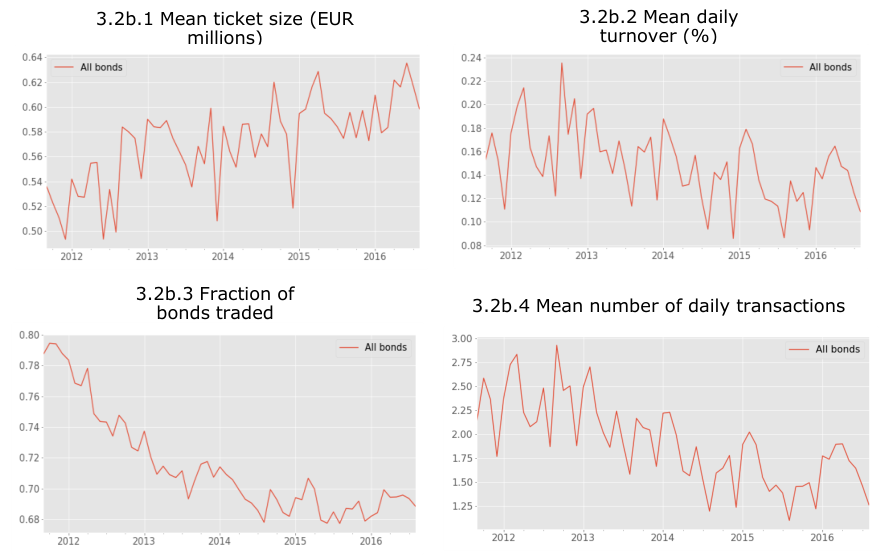
Note: The trends seen in Figure 3.2a become more pronounced when observing only the non-financials. The mean number of transactions for non-financial European corporate bonds has shown a particularly dramatic decline. A decline in mean daily turnover is also noticeable.
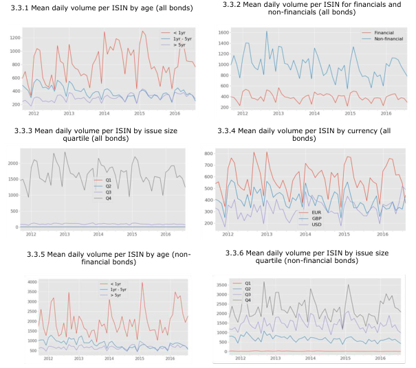
Note: All variables are in EUR thousands. Transaction volume is highest for new issues, non- financials, large issues and euro-denominated bonds.
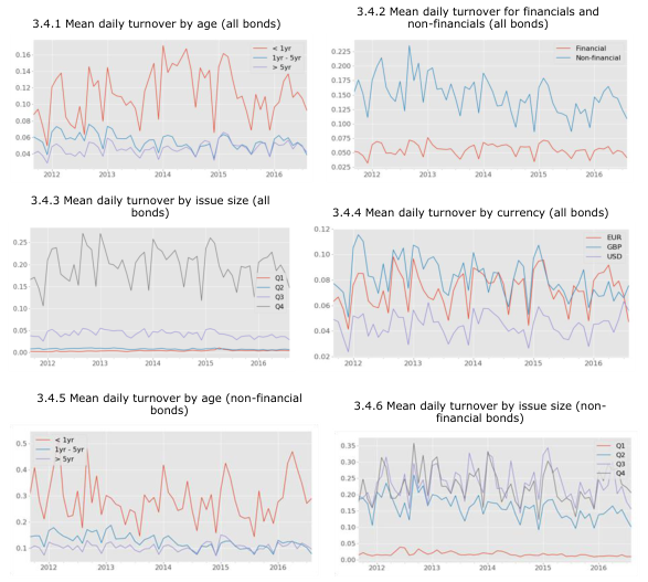
Note: Turnover is measured in percent of the amount outstanding. Turnover is highest for new issues, non-financials, large issues and for Euro and GBP-denominated bonds.
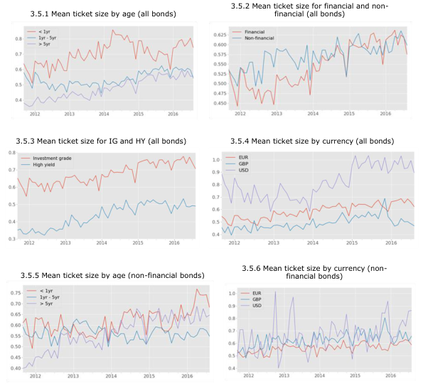
Note: All time series is in EUR millions. Ticket size is largest for new issues, investment grade bonds, and dollar-denominated bonds.
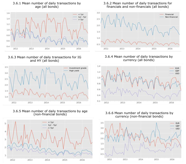
Note: Trading is more active for euro and sterling-denominated bonds, new issues, non-financials and high-yield bonds.
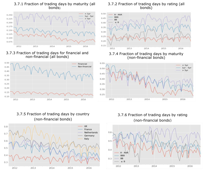
Note: The bonds most likely to trade on a given day are long-term bonds, Italian and German issues (non-financial bonds), and bonds rated BBB or BB. Non-financials are more active, though activity is declining.
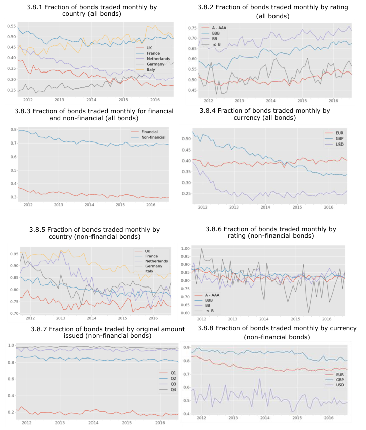
Note: The bonds most likely to trade in a given month are French and Italian, bonds rated BB and BBB, and non-financials. Sterling denominated bonds were initially most active but trading slows over time.
3.3.3 Activity-based indicators from Euroclear ESES data
We now turn to the second dataset that allows one to examine activity-based measures of corporate bond liquidity. The Euroclear ESES data permits one to observe activity at the settlement level. Euroclear has provided data on bond transaction settlements from three distinct reporting units under the Euroclear group umbrella. These constitute three distinct datasets covering distinct segments of the market place. The datasets are available for different time periods which only partially overlap.
Rather than pooling data from different Euroclear entities, we concentrate on the segment which has a wide cross-sectional coverage and the longest time series. This is the Euroclear ESES dataset covering bonds traded in the Euronext group which has branches in France, Belgium and the Netherlands. This provides 32 months of data from January 2014 to August 2016.
In interpreting the data, it is important to bear in mind that transactions are observed at the settlement level. This involves movements between different custodian accounts. Some trades that are made prior to the despatch of a settlement instruction may be netted out.
In the ESES segment, in excess of 800 European corporate bonds typically trade in a given month. Of these, about 500 are financial issues and 300 non-financials. Figure 3.9 shows that the average daily transaction volume in a given bond fluctuated between €300,000 and €700,000 (see 3.9.1). However, issue size has increased so that volume as a fraction of amount outstanding has declined between over the 2014- 2016 period (see 3.9.2).
Figure 3.9.3 suggests that a typical bond is exchanged less than once per day and that this rate (running at about 0.4 transactions per day) declines over the sample period. From Figure 3.9.4, we see that average amounts involved in a single transaction are large, about €4 million. In some months, they are as high as €9 million. This reflects the fact that the data reflects flows between accounts of large institutional entities.
Figure 3.10 gives us further insights into factors that drive differences in activity levels across different categories of bonds. High yield issues tend to trade more frequently than do investment grade (Figure 3.10.1). In Figure 3.10.4, we see that the fraction of bonds traded in a month is highest for bonds rated BB and below. These are both symptoms of a tendency noted above that information sensitive bonds trade more actively than information insensitive bonds.
Figure 3.10.2 provides some confirming evidence supporting another tendency highlighted already. Transaction sizes are much larger for bonds in the first year than for older bonds. This observation is consistent with the notion that young bonds start in the hands of large dealers and progressively gravitate to the portfolios of longer term investors. Finally, we see in Figure 3.10.3 that transaction sizes tend to be significantly larger for financial issues than for non-financials.
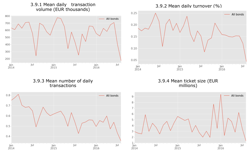
Note: 3.9.1 shows that overall settlement turnover volume is volatile but trendless, while according to 3.9.2 turnover rate per bond has declined. Figure 3.9.3 shows that a typical bond trades less than once per day. It can be seen from 3.9.4 that ticket sizes at the settlement level are significantly higher than at the trade level.
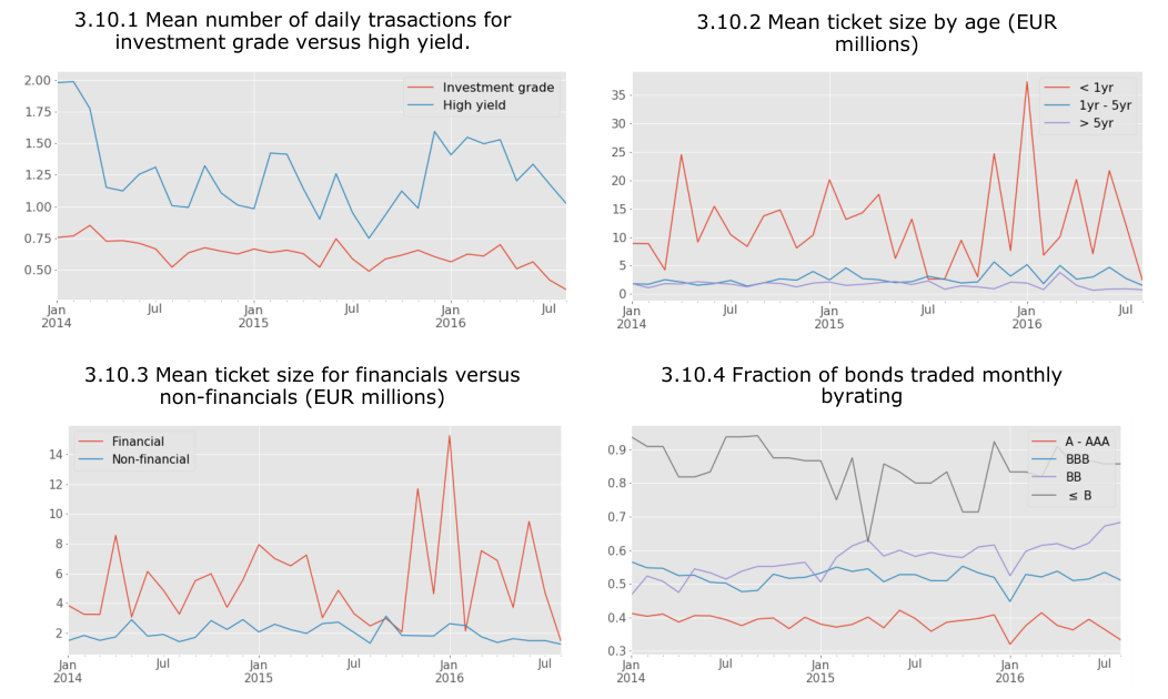
Note: 3.10.1 and 3.10.4 support the notion that high yield bonds are more information sensitive and trade more often. We see from 3.10.2 that dealers trade young bonds in big tickets and from 3.10.3 that financials move in larger lots than non-financials.
3.3.4 Activity-based indicators from a prominent electronic platform
Next, we examine activity in corporate bonds since 2010 from the perspective of a prominent electronic platform that has specialised in client trading with multiple dealers using the RFQ trading protocol. This style of trading will be discussed in greater detail in Section 4 of the report.
Figure 3.11 gives some indicators of overall activity trends on this platform. As one may see from Figure 3.11.1, the number of European corporate bonds traded on the platform have increased from something close to 15,00 in 2010 to about 2,500 in
2014. The number of bonds trading has been steady since then. The FCA dataset had about 4,700 bonds trading in 2014. So the coverage of the platform is now quite extensive. In Figure 3.11.2, we see that the turnover per day per bond rose strongly to about €80,000 per day per ISIN. This number slipped subsequently and has been running at about €60,000 recently.
Comparison between Figure 3.11 and Figure 3.5 suggests that the ticket sizes on platforms tend to be smaller than in bilateral voice market. This is further confirmed in Section 4. However, there has been a noticeable increase in tickets sizes on this platform between 2014 and 2016. This suggests that the slight slippage of average turnover per day per bond has been due to a drop in trading frequency. This is confirmed in Figure 3.11.4 where we see that the fraction of bonds that trade on a given day has declined from about 10% to 7% between 2012 and 2016.
Figure 3.12 gives us some insights into the factors at play behind these trends in platform trading. As seen in Figure 3.12.1, in 2010 and 2011 trades in investment grade issues were more numerous than in high yields. However, numbers of trades in high yields have grown and now stand at similar levels to investment grade. At the same time, the age structure of bonds trading on the platform has evolved, with new issues being trade more actively than previously (Figure 3.12.2).
This suggests that large dealers are beginning to turn to the electronic platform as part of their strategy to distribute bond holdings acquired in the issuance process. In line with this interpretation, we see that the average ticket sizes for newly issued bonds have increased on this platform, again suggestive of a more active involvement of large dealers (Figure 3.12.3). Finally, Figure 3.12.4 gives average numbers of trades per day broken down by rating. From this we see that trading in the information sensitive band of BB to BBB has increased in relative term in recent years.
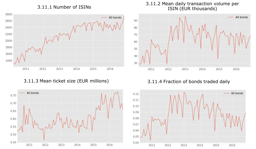
Note: 3.11.1 shows the number of bonds growing to 30% of the market and 3.11.2 shows the turnover per ISIN growing as well. Figure 3.11.3 shows ticket sizes also growing, though they remain small than in big dealer markets. From 3.11.4 we see that generally less than 10% of bonds trade on a given day.
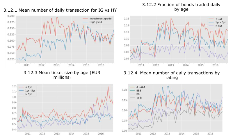
Note: 3.12.1 and 3.12.4 shows the number of trades in high yield and information sensitive BBB and BB bonds growing. Figures 3.12.2 and 3.12.3 show that trading in new issues has grown to be the most active segment, with lots increasing a size of €1 million on average.
3.3.5 Multivariate analysis of activity-based indicators
So far, we have considered what drives changes in observed activity measures of liquidity taking those driving factors one at a time. This has been useful in identifying a number of clear patterns that help to clarify what might be contributing to past trends of liquidity and what might produce changes in the future. However, it may be that not all these factors represent separate influences but rather that one or another may be the primary driver and that, once this is taken into account, the effects of other factors become insignificant. To deal with this issue, we now consider the factors together in a multivariate statistical analysis.
This analysis will also allow us to ask whether the factors we have identified are sufficient to account for the trends that have been identified in overall activity in European corporate bond secondary trading. In particular, do they capture the apparent decline in trading activity that seems to have occurred since 2014?
To address these questions we apply our analysis at the individual security level. For each security we calculate measures of activity monthly. We then pair these with observations of the driving factors associated with the activity variables in the month observed.
We use multiple regression analysis for the following measures of activity: (a) average daily turnover measured as a faction of amount outstanding, (b) average number of transactions daily, (c) the average ticket size and (d) the frequency of trading as measured by the proportion of trading days within a month that the security is traded. Furthermore, we consider a binary indicator variable which equals 1 if the bond does not trade at all in the month and 0 otherwise. This is a strong indicator of whether or not the bond has been distributed into the portfolios of long-term investors who trade only in exceptional circumstances. We use the probit model to study the factors that determine the probability of zero trading.
The explanatory variables that are used to capture driving factors are (i) the logarithm of the age since issuance, measured in years, (ii) the logarithm of the size of issue measured in euros, (iii) a dummy variable capturing whether the issue is a high yield issue or not, (iv) a dummy variable capturing whether security is a financial issue or not, (v) a time trend, (vi) aggregate volatility of all bonds, and (vii) individual volatility.
The results of the regression using the FCA dataset are given in Table 3.5. All regressors employed are demeaned. This implies that the constant equals the unconditional mean of the dependent variable. The time variable is scaled in that the total length of the sample period is assumed to equal one time period. The consequence is that the magnitude of the time trend is transparent. For example, turnover in Panel a) of Table 3.5 has an unconditional mean equal to 0.190. This means that the average daily volume in an individual ISIN is 0.208% of the outstanding par value. Over the five-year sample period, conditional on other influences, the decline in turnover is 0.055, i.e., more than a quarter average turnover.
The results of regressions on all corporate bonds show that the four drivers that we had identified as being important when considered separately are all significant when taken together. The exception is in the transaction frequency regression where both the high yield dummy and the financial dummy are insignificant (as indicated by a tstatistic much less than 2 in absolute value). Otherwise, age, size of issue, financial/non-financial, and HY/IG all have highly significant t-statistics. In the regressions conducted on non-financial corporate bonds, age, size of issue, and HY/IG are all significant except that the HY/IG indicator is not significant when the dependent variable is turnover.
Both age of issue and size of issue have clear effects, both for all corporate bonds and for non-financial bonds only. Age of issue enters negatively and is significant in all the regressions. As the bond ages its turnover, the number trades in a month, its average trade size, and the fraction of days when it trades all decrease. The size of issue enters positively and is significant in all regressions. Turnover rate, numbers of trades, and fractions of days with positive trading are all lower for high yield issues once we have controlled for other factors. Financial issues tend to have higher turnover, larger trade sizes and more transactions than non-financial issues. Transaction frequency is not significantly affected by financial dummy.
We also include as regressors aggregate and individual volatilities. These are estimated by calculating time series standard deviations of daily returns on a rolling basis using, for each month and ISIN, the 30 day period up to the start of that month. In other words, the volatilities are estimated at the ISIN level using a rolling window and are lagged by one month. The individual volatilities are a proxy for the risk of the individual security in question. Risk conditions in the market as a whole may have a separate influence and hence we also include an equally weighted index of the individual volatilities available at any given moment which we refer to as aggregate volatility. The regressions suggest that these volatility variables are significant. Aggregate volatility tends to be associated with lower activity levels whereas individual volatility tends to be associated with higher activity for the bond in question.
Thus, the age of issue, its size, whether or not it is investment grade or high yield and whether it is a financial issue or a non-financial issue are all important determinants of the way a corporate bond trades in the market. The question then becomes whether when taking these determinants into account, do they fully account for the trends we initially noted in activity of bond trading activity since 2000? An answer to this is given by the coefficient of calendar time in the multiple regression of Table 3.5.
For regressions on all corporate bonds and non-financial corporate bonds, the time trend enters negatively and is significant in the regression for turnover, numbers of transactions and for trading frequency. That is, all else equal there has been a deterioration of these measures of activity since 2011. The time trend coefficient is positive and significant in the ticket size regression for both sets of bonds. Thus, the unconditional trends in activity that we noted in Figures 3.1 and 3.3.1 are still present after we control for changing composition in the make-up of the set of bonds trading in the markets.
From our discussion above about the demeaning of regressors and the scaling of time, one may deduce that the economic magnitude of the time effects is considerable for turnover, number of transactions and transaction frequency and somewhat smaller for ticket size. For non-financial bonds (see Panel b) of Table 3.5), the unconditional means for turnover, transaction numbers and frequency are 0.187, 2.141, 0.499, whereas the negative trends over the sample period amount to 0.045, 1.104, and 0.115, which are large in proportional terms.
To examine whether there is evidence that bonds become siloed in long term portfolios, we perform probit analysis of the probability that a bond will not trade in a month using the FCA data. The results of this analysis are presented in Table 3.6. Columns 2 and 3 of the table (in both Panels a) and b)) show results when we use the same explanatory variables as in the regression analyses reported Table 3.5. Age enters positively and is highly significant. That is, the likelihood of a bond being siloed increases as the bond ages, an effect that captures the life-cycle effect that over time a bond is distributed into a number of long-term investor portfolios and remerges into active trading only as an exceptional matter.
Size enters negatively in the model, suggesting that the tendency to be siloed is particularly strong for smaller issues. High yields are more likely to become dormant than investment grade issues and financial issues are more likely to be siloed than non-financial issues. The time trend is positive and significant. That is, over the period from 2011-2016, controlling for all other characteristics the likelihood that a bond will become dormant has risen.
Columns 4 and 5 of Table 3.6 show results when the specification is augmented to include an interaction between age and the time trend. The coefficients for this interaction term are positive while the time trend by itself has become negative. This provides evidence that the deterioration of market liquidity in recent years (as shown by the activity indicators analysed in Table 3.5) has coincided with an acceleration of the life cycle. Bonds are pushed out more rapidly by dealers and arrive earlier at the stage where they are held mostly in portfolios of long-term investors. Otherwise, the effects of issue size, HY/IG, and Financial/Non-financial are the same as in the first specification.
An issue with this probit analysis is that, in most cases, bond-specific volatilities are unavailable for bonds that are very rarely traded. Hence, including volatilities in the probit regression requires dropping many observations, changing the sample substantially. We, therefore, re-ran the probit regressions shown in Table 3.6 excluding the volatility regressors. The results were qualitatively the same as those shown in Table 3.6 except that the constants were much lower reflecting the fact that a large fraction of bonds are not traded within a month.
For these regression we calculated the economic magnitude of the time trend, conditioning on the mean of other independent variables. As all independent variables except the constant are de-meaned in the probit regression, the conditional change in non-trading probability from the start to the end of the period is: , where is the cumulative distribution function of standard normal. Based on the regressions in Table 3.6, the non-trading probability for the FCA dataset increases from 69.76% to 71.92% for all bonds, and increases from 19.82% to 22.57% for non-financial bonds in the period from September 2011 to August 2016. These results combined with those in Table 3.5 constitute evidence that trading activity in European corporate bonds has deteriorated and that this cannot be attributed to the changing composition of the issue types and issuers in the market.
The above analysis makes use of the FCA dataset available to us. We have performed the same multivariate analysis of trading activity using the data provided by Euroclear. In this, we employ the ESES dataset which captures European corporate bond transactions within Euronext. The results are reported in Tables 3.7 and 3.8.
From the regression analysis in Table 3.7 we see that all the driving variables that were significant in the analysis of the FCA are significant here as well. However, the directions of the effects are different in a few cases. Interestingly, the effects of age are now positive in the number of trades and the trading frequency regressions. This may reflect an effect that arises with activity at the settlement level. As a bond ages and is been distributed into the hands of buy-side investors, there may be more investors whose views on returns and other idiosyncratic motives for trading will differ. This might create more movements among trading accounts. However, the amounts moved and the size of movements may decline with age.
Turning to the time trend we find, for the Euroclear data (as for the FCA data), a negative coefficient for turnover, number of transactions, and transaction frequency. All these effects are statistically significant and they appear economically important of one compares the time coefficients with the constants (which equal the unconditional means of the dependent variables). Here, we find no significant time effect in the ticket size regression. Thus, in both the FCA regressions and the Euroclear dataset, controlling for other factors, it appears that there a marked contraction in trading activity as measured by several statistics, has occurred.
Finally, Table 3.8 presents probit analysis of the probability of zero trades in a month using Euroclear ESES data. Age, issue size, the high yield dummy and the financial issue dummy are all significant. The effect of time is similar to that found in the FCA data. In the first specification, in which time enters alone, the time trend is positive and significant. That is, other things equal, it becomes increasingly likely that a bond will be siloed. In the second specification, time by itself is negative and significant, but, when an interaction with age is included, it is positive and highly significant. Our interpretation of this is the same as in the case of the FCA data. It is evidence of a compression of the life cycle of bonds as dealers push the distribution of bonds into stable hands at a faster rate.
Again, we calculate the economic magnitude of the time trend. The probit regressions in Table 3.8 do not include volatility so there is no issue of dropping observations for which bond specific volatilities are unavailable (as there was for the FCA data probit analysis). We calculate, for the regression in Table 3.8 without the interaction effect, that the non-trading probability for the Euroclear ESES dataset increases from 59.52% to 68.00% in the period from January 2014 to August 2016.
| Number of | Ticket | size | Transaction | |||||
|---|---|---|---|---|---|---|---|---|
| Turnover | (%) | transactions | (EUR | millions) | frequency | |||
| Dependent variable | Coeff. | t-stat. | Coeff. | t-stat. | Coeff. | t-stat. | Coeff. | t-stat. |
| Constant | 0.208 | 52.2 | 2.374 | 54.3 | 0.666 | 198.9 | 0.510 | 126.0 |
| Log age | -0.090 | -16.2 | -0.751 | -15.7 | -0.117 | -30.6 | -0.079 | -26.0 |
| Log size | 0.035 | 19.0 | 1.040 | 14.4 | 0.304 | 66.2 | 0.161 | 53.3 |
| High yield dummy | 0.009 | 5.1 | 0.325 | 12.3 | -0.052 | -29.9 | -0.002 | -0.8 |
| Financial dummy | 0.027 | 8.6 | 0.295 | 10.5 | 0.075 | 9.9 | 0.003 | 1.0 |
| Aggregate vol | -0.009 | -2.7 | -0.058 | -1.4 | -0.001 | -0.6 | -0.002 | -0.5 |
| Individual vol | 0.003 | 4.4 | 0.039 | 4.7 | -0.002 | -3.0 | 0.000 | -0.1 |
| Time | -0.055 | -3.0 | -1.317 | -6.3 | 0.164 | 13.0 | -0.133 | -6.9 |
| Number observations | 132,073 | - | 144,719 | - | 132,073 | - | 144,719 | - |
| Number months | 60 | - | 60 | - | 60 | - | 60 | - |
| Adjusted R-sq. | 0.09 | - | 0.10 | - | 0.16 | - | 0.21 | - |
| F-stat. | 108.9 | - | 51.7 | - | 2,278.0 | - | 807.4 | - |
| Panel b) Non-financial | Bonds | |||||||
| Number of | Ticket | size | Transaction | |||||
| Turnover | (%) | transactions | (EUR | millions) | frequency | |||
| Dependent variable | Coeff. | t-stat. | Coeff. | t-stat. | Coeff. | t-stat. | Coeff. | t-stat. |
| Constant | 0.187 | 44.7 | 2.141 | 49.9 | 0.601 | 165.3 | 0.499 | 96.5 |
| Log age | -0.065 | -17.3 | -0.604 | -12.4 | -0.042 | -8.8 | -0.069 | -31.1 |
| Log size | 0.033 | 11.9 | 1.262 | 16.5 | 0.198 | 43.3 | 0.240 | 61.2 |
| High yield dummy | 0.000 | 0.1 | 0.300 | 9.1 | -0.064 | -26.4 | 0.012 | 4.4 |
| Aggregate vol | -0.004 | -1.2 | -0.033 | -1.0 | -0.006 | -2.8 | 0.004 | 0.8 |
| Individual vol | 0.002 | 2.3 | 0.033 | 2.3 | 0.003 | 1.9 | -0.001 | -1.4 |
| Time | -0.045 | -2.6 | -1.104 | -6.1 | 0.057 | 3.9 | -0.115 | -6.1 |
| Number observations | 40,067 | - | 43,981 | - | 40,067 | - | 43,981 | - |
| Number months | 60 | - | 60 | - | 60 | - | 60 | - |
| Adjusted R-sq. | 0.06 | - | 0.09 | - | 0.09 | - | 0.31 | - |
| F-stat. | 89.3 | - | 73.5 | - | 517.6 | - | 1,412.6 | - |
Note: The regressions are estimated using Ordinary Least Squares. Standard errors are robust to time-specific clusters and serial correlations of two lagged periods (See Annex 6 for methodology). These tables show the results of estimating regressions for different activity variables. All independent variables are monthly averages per ISIN. Turnover is the average daily turnover rate within a month in percent. Number of transactions is the average daily number of transactions within a month. Ticket size is the average size of transaction within a month in million EUR. Transaction frequency is the fraction of days within a month for which there is at least one transaction. All dependent variables except the constant are demeaned. The time variable is scaled so that the difference in its value from the start to the end of sample period equals unity.
| Dependent variable | Coeff. | t-stat. | Coeff. | t-stat. |
|---|---|---|---|---|
| Constant | -1.576 | -264.371 | -1.576 | -264.4 |
| Log age | 0.195 | 25.4 | 0.168 | 9.1 |
| Log size | -0.622 | -103.3 | -0.622 | -103.3 |
| High yield | 0.252 | 41.1 | 0.252 | 41.1 |
| Financial | 0.084 | 7.3 | 0.085 | 7.3 |
| Aggregate Vol | 0.000 | -0.1 | 0.000 | -0.1 |
| Individual Vol | 0.003 | 6.7 | 0.003 | 6.8 |
| Time | 0.160 | 7.0 | 0.091 | 1.9 |
| Log age X time | - | - | 0.001 | 1.6 |
| Number observations | 144,719 | - | 144,719 | - |
| Number months | 60 | - | 60 | - |
| Pseudo R-sq. | 0.18 | - | 0.18 | - |
| Panel b) Non-financial | bonds | |||
| Probability of no | transaction | |||
| Dependent variable | Coeff. | t-stat. | Coeff. | t-stat. |
| Constant | -1.833 | -132.087 | -1.833 | -132.0 |
| Log age | 0.073 | 4.4 | -0.046 | -1.2 |
| Log size | -1.166 | -73.9 | -1.165 | -73.8 |
| High yield | 0.227 | 18.8 | 0.228 | 18.9 |
| Aggregate Vol | -0.008 | -0.8 | -0.008 | -0.9 |
| Individual Vol | 0.003 | 4.1 | 0.003 | 4.1 |
| Time | 0.228 | 4.8 | -0.070 | -0.7 |
| Log age X time | - | - | 0.004 | 3.5 |
| Number observations | 43,981 | - | 43,981 | - |
| Number months | 60 | - | 60 | - |
| Pseudo R-sq. | 0.38 | - | 0.38 | - |
Note: These tables show the results of estimating regressions for a dummy variable taking the value 1 only when no trade occurs for the specified bond in the specified month, and 0 otherwise. All independent variables except the constant are demeaned. The time variable is scaled so that the difference in its value from the start to the end of sample period equals unity.
| Number of | Ticket | size | Transaction | |||||
|---|---|---|---|---|---|---|---|---|
| Turnover | (%) | transactions | (EUR | millions) | frequency | |||
| Dependent variable | Coeff. | t-stat. | Coeff. | t-stat. | Coeff. | t-stat. | Coeff. | t-stat. |
| Constant | 0.873 | 46.6 | 0.585 | 48.8 | 4.005 | 16.1 | 0.141 | 78.2 |
| Log age | -0.776 | -13.5 | 0.098 | 4.5 | -6.115 | -10.0 | 0.030 | 5.6 |
| Log size | -0.199 | -6.8 | 0.208 | 22.5 | 1.027 | 3.8 | 0.043 | 38.0 |
| High yield dummy | -0.251 | -7.8 | 0.120 | 8.6 | -0.515 | -1.5 | 0.020 | 10.7 |
| Financial dummy | 0.558 | 12.3 | 0.213 | 21.8 | 4.823 | 7.3 | -0.025 | -8.1 |
| Time | -0.270 | -4.1 | -0.311 | -6.1 | 0.885 | 1.1 | -0.060 | -8.1 |
| Number observations | 25,484 | - | 67,249 | - | 25,530 | - | 67,249 | - |
| Number months | 32 | - | 32 | - | 32 | - | 32 | - |
| Adjusted R-sq. | 0.04 | - | 0.04 | - | 0.02 | - | 0.10 | - |
| F-stat. | 72.0 | - | 443.9 | - | 38.8 | - | 934.8 | - |
Note: Estimated by Ordinary Least Squares with standard errors robust to time-specific clusters and serial correlations of 2 lagged periods (See Annex 6 for methodology). All dependent variables are monthly averages per ISIN. Turnover is the average daily turnover rate within a month in percent. Number of transactions is the average daily number of transactions within a month. Ticket size is the average size of transaction within a month in million EUR. Transaction frequency is the fraction of days within a month for which there is at least one transaction. All independent variables except the constant are demeaned. The time variable is scaled so that the difference in its value from the start to the end of sample period equals unity.
| Probability | of no | transaction | ||
|---|---|---|---|---|
| Dependent variable | Coeff. | t-stat. | Coeff. | t-stat. |
| Constant | 0.356 | 67.8 | 0.357 | 67.8 |
| Log age | -0.147 | -18.9 | -0.321 | -21.3 |
| Log size | -0.247 | -71.2 | -0.250 | -71.6 |
| High yield | -0.073 | -11.9 | -0.074 | -12.0 |
| Financial | 0.449 | 38.9 | 0.448 | 38.8 |
| Time | 0.234 | 12.8 | -0.273 | -6.6 |
| Log age X time | - | - | 0.011 | 13.5 |
| Number observations | 67,249 | - | 67,249 | - |
| Number months | 32 | - | 32 | - |
| Pseudo R-sq. | 0.11 | - | 0.11 | - |
Note: These tables show the results of estimating regressions for a dummy variable taking the value 1 only when no trade occurs for the specified bond in the specified month, and 0 otherwise. All independent variables except the constant are demeaned. The time variable is scaled so that the difference in its value from the start to the end of sample period equals unity.
3.4 Price-based indicators of European corporate bond liquidity
3.4.1 Bloomberg Bid-ask Spreads
We now turn to consider price-based indicators of liquidity. The most obvious of these is bid-ask spreads for individual bonds. Based on quotes, such spreads may be criticised as being non-executable expressions of trading interest. Nevertheless, they have the advantage that they are observable over long periods of time for a large fraction of the market. They are also quite closely correlated with other price measures of liquidity like effective spreads. The Bloomberg spreads that we employ in this section comprise 7,000 ISINs and amount to €3.5 trillion in value outstanding by the end of the sample period.
Figure 3.13 contains plots of the evolution of spreads over time. For each plot, we calculate average spreads for each bond within a given month and then average over the bonds in a specific category for which spreads are available in that month.
It is noticeable from Figure 3.13 that the first stage in the financial crisis (which occurred in 2007-8) had little impact on European corporate spreads. A moderate peak is visible following the Lehman Brothers failure in early 2009. The major spike in European corporate bond spreads only occurs when concerns mount about the credit standing of European sovereigns and a possible disintegration of the Euro in 2011.
In Figure 3.13.1, one may observe that spreads fell back substantially in 2012 and 2013 as central banks took firm action to resolve the crisis. Spreads overall remain above pre-crisis levels, however, and a moderate upward trend is apparent from early
2014. Bond spreads for financial and non-financial issuers have moved closely together except at the height of the 2011 crisis when spreads for Financials understandably rose to higher levels (see 3.13.2).
The distribution of spreads across different bond categories apparent in Figure 3.13 reflected intuitively reasonable patterns. New bonds exhibit lower spreads than old (see 3.12.3). This is consistent with activity-based indicators viewed above which show that young bonds trade more frequently. If market makers face inventory costs, faster bond turnover will imply lower costs.
Bid-ask spreads for investment grade bonds are noticeably lower than those of high yield bonds. Again, this is consistent with a dealer inventory-cost view of market making as HY bond positions are riskier than IG issues. It is also noteworthy that the sensitivity of spreads to factors that drive risk like HY versus IG is greater since the crisis than before. Between 2004 and 2009, bid-ask spreads for HY and IG appear quite close whereas since the crisis the former are much higher.
Figure 3.14 shows further breakdowns of Bloomberg spreads over time. The spreads exhibit a clear issue-size effect during and following the crisis. Spread averages for quartiles of the sample categorised by issue size (labelled as “Q1”, “Q2”, etc., in Figure 3.14.1) are monotonic in issue size with the small issue bonds (labelled “Q1”) exhibiting the highest spreads. This is in contrast to behaviour one may observe before the crisis in that prior to 2011, the quartile averages were not monotonically decreasing in issue size.
The spreads for bonds categorised by currency show that GBP bonds have the highest spreads in most periods with spreads on Euro-denominated bonds only matching them at the height of the crisis. This tendency for trading costs to be higher for GBP issues than for EUR issues was one of the findings in Biais et al. (2006). Perhaps controversially, they attributed this finding to a more competitive market structure in market making for continental European issues than for sterling denominated corporate bonds.
The above discussion highlights how issues of risk and liquidity are interwoven in interpreting spread levels. Clearly, liquidity drivers like issue size and age affect spreads. Yet the simple riskiness of the securities is also a crucial driver of spread magnitudes. Much of the discussion of liquidity in the regulatory studies summarised in Section 2 fails to differentiate between these two factors. So far, in this section, we have done the same.
How can one untangle the relation between risk and liquidity to elicit from bid-ask spread data how liquidity-related premiums affect the costs of trading? One way is to calculate spreads holding risk constant. To achieve this, for every bond ISIN and every day, we estimate the annualised return volatility based on bond mid-prices (inferred from Bloomberg bid and ask prices) using the previous 30 days of data. Running forward through the sample, one may then categorise individual bonds into one of several buckets based on these volatilities and calculate the average spreads for all the days in a month and for all the bonds in the relevant bucket. The volatility buckets we employ correspond to volatility ranges from 0 to 2.5% annualised, 2.5 to 5%, 5 to 10%, and more than 10%.
Figure 3.14.3 shows time series of average spreads for bonds bucketed based on lagged price volatility (calculated as just described). These suggest a very different dynamic of spreads than that found in the principal regulatory studies surveyed in Chapter 2 and, indeed, from that shown in Figures 3.13.1 to 3.14.2. In particular, we see that conditional on volatility the bid/ask spreads rose sharply with the onset of the sovereign debt crisis in Europe and have persisted at these high levels, admittedly with rather wide fluctuations.
Thus, the general recovery of spreads found in the studies surveyed in Chapter 3 may, in part, be attributable to the decline in volatility since 2012. Indeed, as is seen in Figure 3.14.4, most of the trading activity has reverted to securities in the low volatility range. These results suggest that the capacity of the market to intermediate transactions in instruments of homogeneous risk might have changed structurally since the crisis.
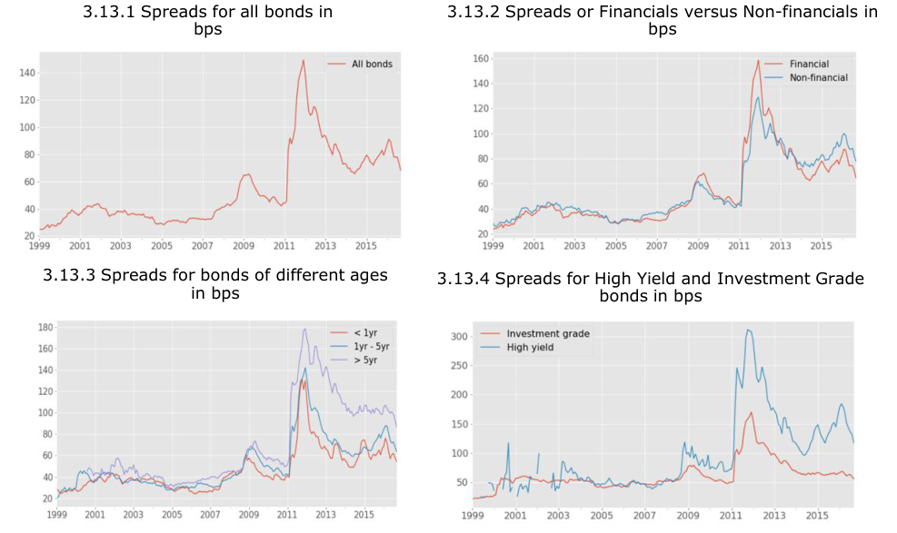
Note: Bid-ask spreads are highest for financials, older bonds and high-yield bonds. Spreads spike in 2011 with the intensification of concerns about European sovereign debt. Thisspike is most pronounced for high-yield bonds which carry a more significant risk of default.
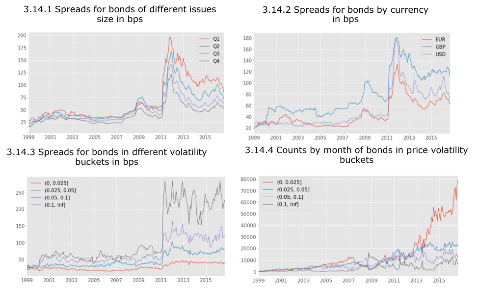
Note: Bid-ask spreads are highest for small issues, sterling-denominated bonds and more volatile bonds. Furthermore, the high bid-ask spreads post-crisis are persistent in each volatility bucket.
3.4.2 Effective spreads
Another measure of cost of trading may be inferred from the data provided by a prominent Electronic Trading Platform (ETP). From this data, one may calculate Effective Spreads defined as the absolute gap between transactions prices and the contemporaneous (intraday) mid-price. The latter is measured by the platform itself using quotes from multiple dealers.
We have calculated the effective spreads for individual transactions and then have averaged them over months for the market as a whole and for subsets of ISIN’s sorted into difference categories. The monthly averages of ISIN Effective Spreads for different categories of bonds are shown in Figures 3.15 and 3.16.
Figure 3.15.1 shows the evolution over time of Effective Spreads for all the bonds. The pattern of the Effective Spreads, which is shown for 2010 onwards, is quite similar to that of the Bloomberg bid-ask spreads. Both exhibit similar peaks in late 2011 and then, following a large drop, a moderate tendency to increase after 2014.
One may expect that Effective Spreads will be of the order of half the full spread between buying and selling transactions prices as they equal the distance from midprice to transactions prices. Comparing the data in Figure 3.15.1 with those in Figure 3.13.1, one may observe that the Effective Spreads are noticeably lower than half the Bloomberg bid-ask spreads. This suggests that the ETP trading occurs well within the bid-ask spread as shown on Bloomberg. This comparison is rough since we have not taken into account possible differences in the composition of the sets of bonds employed in the two spread calculations presented here.
From Figure 3.15.2, as with the Bloomberg data, financials exhibit higher spreads during and immediately after the crisis, but the discrepancy has dissipated more recently. Spreads by age, as was the case with the Bloomberg spreads, show greater magnitudes for older bonds (see 3.15.3). High yield bonds exhibit spreads of greater magnitude during and since the crisis, as was also true for the Bloomberg spreads (see 3.15.4).
Figure 3.16 shows breakdowns of the ETP Effective Spreads using additional categorisations. Figure 3.16.1 shows Effective Spreads by issue size. Again, the bonds are categorised by issue size into quartile groups with Q1 denoted the smallest and Q4 indicating the largest issue size bonds. As with the Bloomberg data, the Q1 spreads are highest and the Q4 spreads are the lowest. Figure 3.16.2 shows spreads by currency. The spreads for Euro-denominated bonds are consistently lower than those of GBP-denominated bonds.
Figure 3.16.3 shows ETP Effective Spreads bucketed by mid-price volatility. The volatility data employed is calculated using Bloomberg mid-prices. (It was not possible to estimate mid-price time series from the ETP transactions prices themselves because of the infrequency with which bonds are traded.) The striking aspect of the plot in 3.16.3 is the fact that the 2011 crisis-related peak in the time series is largely flattened out. The post 2014 upward drift in spreads is not much more pronounced than the spreads for all the bonds but the peak associated with the crisis is removed.
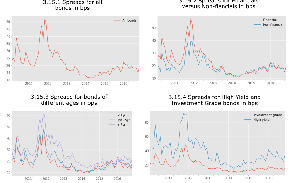
Note: Effective spreads are highest for financials, older bonds and high-yields bonds. This is consistent with observations of the bid-ask spread in Figure 3.13. Effective spreads spike at a similar time to the bid-ask spreads, and the spike is similarly more pronounced for high-yield bonds.
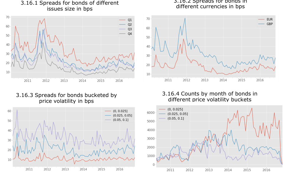
Note: Effective spreads are highest for small issues, sterling-denominated bonds and more volatile bonds. Furthermore, the high bid-ask spreads post-crisis are persistent in each volatility bucket. This is consistent with Figure 3.14. Bucketing by volatility removes the post-crisis spike.
3.4.3 Price impact liquidity indicators
The last set of liquidity indicators here considered are price impact measures and other measures of trading costs based on short-term prices changes. These include Amihud ratio measures, the Roll measure (introduced by Richard Roll and employed recently in the context of corporate bond liquidity by Bao, Pan, and Wang (2011)), and Imputed Round-trip Costs measure (IRTC). These measures were implemented in one form or another in the three principal regulatory studies surveyed in Chapter 2 of this report.
These measures were originally introduced for the analysis of trading costs in equity markets. Given this origin, one might argue that they were designed for use in the markets, like the equity market, in which trading occurs continuously. Adapting these measures to the world of corporate bonds where for trading for most issues is extremely sparse is not straightforward. We explain the approach that we take to this issue in some detail below.
We implement three versions of the Amihud ratio. The first measure may be defined as , for a given day t and bond j, equals the average follows. The ratio, denoted (over individual transactions) of the ratio of the absolute return between any two successive transactions and the volume of the second of the pair of transactions. The idea is to capture how much volumes of trades translate into price volatility.[32] Note that this measure is available only on days when security j trades at least twice. Days when this does not happen are missing observations (rather than zeros).
. This is The analysis below will make use of a monthly Amihud measure, calculated as the arithmetic average of the daily observations (the sum of divided by the number of days when the measure is available. If there available are no days in the month when there were at least two transactions then the monthly Amihud measure is missing data for that month.[33] The overall market Amihud measure in month m is the arithmetic average of the over all ISINs. This is denoted and is referred to in what follows as Amihud measure 1.[34]
An alternative implementations of the Amihud is proposed in the book by Foucault, Pagano and Roell. They define the Amihud ratio as the ratio of the absolute daily return on the security divided by the total volume transacted in the day.[35] Amihud (and Foucault, Pagano and Roell) have in mind using this with stock market data where the daily return could be measured as the one day change in log prices (close to close) and the denominator is just the volume on the day. One may implement the measure only on days for which the volume of bond trading exceeds zero and for which a closing price is available for the preceding day.[36] This second Amihud measure is referred to in what follows as Amihud measure 2.
- FCA data
Note that there are yet more versions of Amihud-type indicators. For example, AMF that the authors
(2015) implements a price impact measure (here denoted as refer to as an Amihud ratio which consists for a given bond and given day of the ratio of the standard deviation of intraday returns on the bond divided by the square root of the sum of the volumes of trades in the day.[37] Again, this can be calculated only on days with at least two transactions. This last Amihud measure is referred to in what follows as Amihud measure 3.
From Figure 3.17.1 we see that there is a distinct pattern of rise in measured price impact that rose between 2013 and the beginning of 2015. Following a sharp subsequent drop the measure has shown a consistent rising trend from the second quarter of 2015 and through 2016.
From Figure 3.17.2 we see that the sharp drop in early 2015 was associated mostly with non-financial issues. From Figures 3.17.3 and 3.17.4 we see that this pattern held for bonds of all ages and for both investment grade and high yield bonds.
- FCA data
Figure 3.19 presents the results obtained using the Amihud ratio implemented using intraday volatility as a proxy for return as in the AMF (2015) study. The pattern is broadly similar to the previous two sets of results in that there is a perceptible increase in measured price impact between 2014 and 2016. This holds for bonds of all ages and for both financial and non-financials. The increase in price impact appears to be felt most for HY.
- FCA data
Figure 3.18 presents time series plots of Amihud ratios employing the measure based ). By this measure we see a clear decline in price impact between on daily returns ( 2011 and 2013 and then a subsequent increase through 2016. This holds for all bonds and also for bonds broken down by age, HY/IG and financial/non-financial.
The next liquidity measure presented is the Roll statistic. This is based on estimates of the autocovariance of returns over successive periods. Here, it is implemented using the autocovariance of daily returns in a security with a given month.[38]
This measure is effectively trying to infer trading costs from the bid/ask bounce of successive transactions. By design it is most amenable to trading in high frequency environments where the time delay between successive transactions is very short and the chance that a significant piece of news arrives is small. Obviously this is not a set of conditions that is fulfilled in the European corporate bond market. Therefore we include this measure simply for completeness and comparability to previous studies.
The results in Figure 3.20 show that starting from initially high levels of the BPW measure (i.e., high illiquidity) in 2012 the measure declined to moderate levels by 2013 and have been relatively stable thereafter. This holds for financial and nonfinancials. It seems that this movement is a phenomenon affecting older bonds and high yield issues, i.e., the bonds that naturally are the least liquid.
Finally, we implement the IRTC measure without dealer/client identifiers. This methodology was developed by Feldhütter (2012). It is motivated by his observation that in TRACE data for US corporate bonds, one may observe periods of no trading in a given security followed by multiple trades over a short time interval. Feldhütter interprets this as an occurrence of a client-initiated trade after which the dealer lays off the exposure to other dealers. Eventually, dealers return to a flat book via a second client-initiated trade. Feldhütter assumes that the highest trade price in this sequence is the client buy and the lowest price in this sequence is the client sell.[39]
38 Let the arithmetic average of transaction prices in security j on day t. Then the daily return
of security j on day t is if and exist. The Roll measure for security j in that is, minus the covariance of daily returns in the month. month m is One can summarize this measure for the market as a whole by calculating the arithmetic average of for all ISIN j. Call this
This measure can be calculated only when we have sequences of at least 2 days when one has well-defined bond returns in the month. For example, suppose in one month there are returns on 8 days as follows: . The mean return in the month is: ( 2 , 3 , 4 , 7 , 8 , 9 , 10 , 13 )/8 . Then, the covariance of returns is calculated using returns on successive days. This gives: 4 + 7 × 8 + 8 × 9 + 9 × 10 /5.
39 So, the Imputed Round-trip Cost is calculated as
(3.4)
is the minimum Here, is the maximum transaction price in the k’th client chain and is transaction price in the k’th client chain. We only select chains for which: . the total number of non-zero implicit client chains in security j on day t,
In our study, we define an imputed client chain as a case where there are at least two trades with transaction amount difference no larger than 0.5 million EUR occur within 3 hours’ time interval on a given day. We compute the monthly implicit trading cost in security j in month m as the arithmetic average of non-zero Averaging across ISINs, we obtain and aggregate measure denoted .
Figure 3.21 presents the results based on the Imputed Round-trip Cost measure. From Figure 3.21.1 we see a clear down trend between 2011 and 2014 and a clear rise from 2015 to 2016 (of about 8 basis points). This is similar to the pattern noted for bid-ask spreads, Effective Spreads, and the Amihud measure based on daily returns. It applies to financials and non-financials (see 3.21.2), to all ages (see 3.21.3) and to both HY and IG (see 3.21.4). These observations point to a decline in market liquidity since 2014.
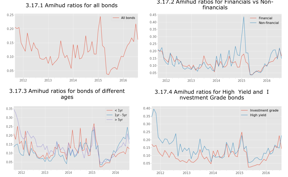
Note: For each month, top 1% observations are winsorized. Amihud measure 1 rose steadily from 2013 to 2015, where it dropped significantly. This drop is most noticeable for non- financials. It has since risen to a similar level to the 2015 peak.
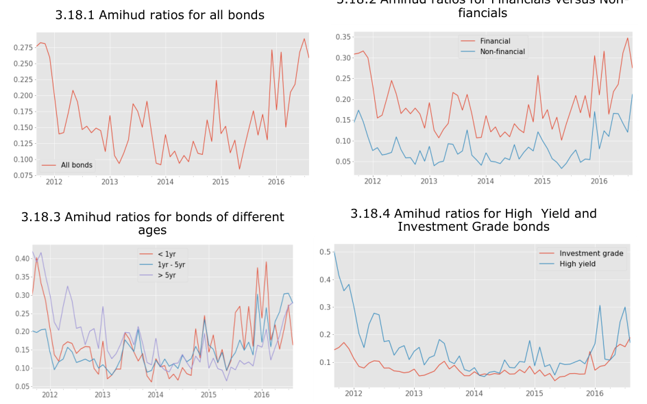
Note: For each month, top 1% observations are winsorized. Amihud measure 2 declines from 2011 to early 2013 and begins to rise in mid-2015. Amihud measure 2 is highest for financials and high-yield bonds.
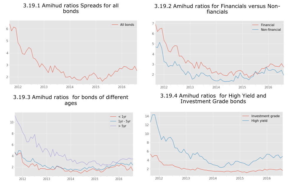
Note: For each month, top 1% observations are winsorized. Bond age impacts Amihud measure 3 more noticeably, with older bonds exhibiting higher Amihud ratios.
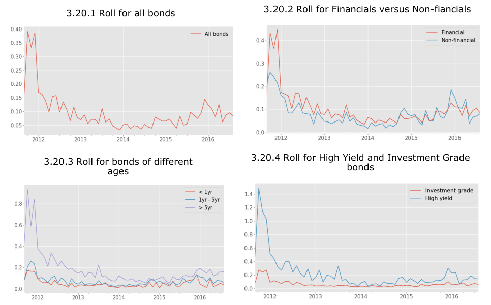
Note: For each month, top 0.5% and bottom 0.5% observations are winsorized. The Roll measure shows a spike in 2011, after which it slowly levels out. The Roll measure is highest for financials, older bonds and high-yield bonds; this indicates lower levels of liquidity.
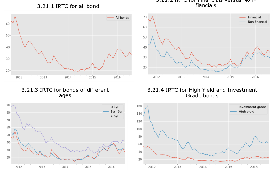
Note: For each month, top 1% observations are winsorized. The imputed round-trip cost declines until 2015, when it begins to rise steadily. This trend is comparable to Amihud measures 2 and 3. The imputed round-trip cost is highest for financials, older bonds and high-yield bonds.
3.4.4 Multivariate analysis of price-based liquidity indicators
As with the quantity-based indicators, one may obtain additional insights about the price-based indicators by performing multivariate, panel regressions. We are interested in the time trends exhibited by these indicators holding constant bond characteristics and risk. All the price-based indicators that we have examined follow u-shaped time paths following the crisis. The Bloomberg bid-ask spreads are available for a longer sample period and are low before the crisis occurs.
Table 3.9 presents regression analysis of the ISIN-level Bloomberg bid-ask spreads. The dependent variable is monthly averages of bid-ask spreads for each ISIN. The independent variables are the same characteristics used in earlier regressions including
ISIN level and aggregate (averaged across ISINs) measures of return volatility (based on returns over a 30-day window finishing on the last day of the previous month).
The regression results are in most cases intuitive in the signs of the effects. Increases in age enter positively and are significant. The coefficient on size is negative and significant. The financial dummy is negative and significant. The HY dummy enters negatively which is counter-intuitive. The individual volatility measure enters positively as expected and is highly significant.
Once we control for these determinants the remaining variation is captured by a time trend which is positive and highly significant for the sample as a whole. For the shorter sample period, the time variable is significant positive for non-financials but not significant for corporate bonds as a whole. This is additional supporting evidence in support of the interpretation we have advanced above. Once we control for changes in underlying volatility, issuer characteristics and issue characteristics, we find evidence of the deterioration of liquidity in the European corporate bond market over time.
Table 3.10 presents regression analysis of the ETP Effective Spreads. Also, shown are results for the bid-ask spreads recorded on the ETP at the same times as the transactions. Again, the results are similar to those obtained using Bloomberg spreads. The regressors are highly significant and have intuitively reasonable signs. Log age, the high yield dummy, the financial dummy and volatility all have positive signs while the log issue size has negative signs.
One difference between Tables 3.9 and 3.10 is that, for all corporate bonds, the time trend enters negatively in the ETP results. The level of statistical significance for the negative parameter is rather low. For non-financial bonds, the time trend is positive although, again, it is not significant. The regression does not provide clear evidence of a trend change, either positive or negative, in structural liquidity. Inspection of Figure 3.16.4 suggests that, bucketed by volatility, effective spreads exhibit a faint U-shape with a moderate rise from 2014 onwards. These shapes are hard to capture with a linear regression and the dynamics may reflect changes in ETP trading associated with a deepening in the market as volumes increased.
In particular, as we shall document in the next section, the market share of RFQ platforms grew sharply between 2010 and 2014 and has been fairly steady since then. This is symptomatic of a maturing of the RFQ product, an observation that we will explore in some detail in Chapter 4. With this maturing it is likely that competitive pressure has increased. This may be due to either increased participation of dealers on a given platform or through entry by new platforms seeking to take market share from earlier entrants or both. These pressures could have been reflected in tighter pricing all else equal, thus showing up as a negative spread in the ETP regressions in Table 3.10.
The magnitudes of the coefficients for the Effective Spreads are about a quarter of the size of those for bid-ask spreads but are otherwise fairly consistent in relative magnitude across the Effective Spreads and the Bid-Ask Spreads. There is more variation across the coefficients obtained in the ETP Bid-Ask Spread regressions (see the left hand column of Table 3.10) and those obtained in the equivalent Bloomberg spread regressions (see Table 3.9). This likely reflects the fact that the Bloomberg spread regressions are based on a much longer time period, although for some variables like High Yield dummy the coefficients are similar in magnitude.
Finally, Table 3.11 presents regression results for the market depth indicators and the simplified round trip return indicator, IRTC. For the Amihud ratios, the time trends are mostly positive, with the exception of Amihud2 for all bonds. . The two cases in which the coefficients are strongly significant, the time trend is positive. Since the unconditional averaged indicators are u-shaped over time, it is noteworthy that the conditional time trends are mostly positive. Again, the time trends shown in the regressions are positive and significant. Finally, the IRTC measures show positive time trend holding other influences constant according to the regression analysis.
| Panel a) | 01/1999 to 09/2016 | ||||
|---|---|---|---|---|---|
| All corp | bonds | Non-financials | |||
| Dependent | variable | Coeff. | t-stat. | Coeff. | t-stat. |
| Constant | 68.154 | 29.104 | 70.225 | 37.774 | |
| Log age | 14.503 | 12.0 | 8.512 | 6.9 | |
| Log size | -10.290 | -12.4 | -20.153 | -15.0 | |
| High yield | dummy | -1.845 | -1.0 | -4.804 | -4.0 |
| Financial | dummy | -1.573 | -1.5 | - | - |
| Aggregate | Vol | -2.033 | -2.9 | -2.022 | -1.7 |
| Individual | Vol | 3.925 | 5.2 | 4.330 | 5.2 |
| Time | 67.623 | 14.1 | 66.405 | 14.2 | |
| Number | observations | 344,168 | - | 98,122 | - |
| Number | months | 213 | - | 213 | - |
| Adjusted | R-sq. | 0.24 | - | 0.31 | - |
| F-stat. | 129.5 | - | 143.2 | - | |
| Panel b) | 01/2010 to 09/2016 | ||||
| All corp | bonds | Non-financials | |||
| Dependent | variable | Coeff. | t-stat. | Coeff. | t-stat. |
| Constant | 78.134 | 32.742 | 79.933 | 40.758 | |
| Log age | 18.709 | 17.0 | 12.055 | 11.0 | |
| Log size | -14.216 | -12.8 | -25.621 | -15.8 | |
| High yield | dummy | -1.132 | -0.6 | -6.689 | -4.9 |
| Financial | dummy | 2.183 | 1.8 | - | - |
| Aggregate | Vol | 1.182 | 0.5 | 0.922 | 0.5 |
| Individual | Vol | 6.588 | 8.9 | 5.695 | 4.5 |
| Time | 15.137 | 1.3 | 17.185 | 1.8 | |
| Number | observations | 253,477 | - | 73,816 | - |
| Number | months | 81 | - | 81 | - |
| Adjusted | R-sq. | 0.33 | - | 0.35 | - |
| F-stat. | 305.7 | - | 214.4 | - |
Note: Estimated by Ordinary Least Squares with standard errors robust to time-specific clusters and serial correlations of 2 lagged periods (See Annex 6 for methodology). Dependent variable is bid-ask spread in basis point. All independent variables except the constant are demeaned. The time variable is scaled so that the difference in its value from the start to the end of sample period equals unity.
| All corp | bonds | Non-financials | ||
|---|---|---|---|---|
| Dependent variable | Coeff. | t-stat. | Coeff. | t-stat. |
| Constant | 13.162 | 44.0 | 12.911 | 40.6 |
| Log age | 2.603 | 13.8 | 0.676 | 3.1 |
| Log size | -4.468 | -14.0 | -4.723 | -11.5 |
| High yield dummy | 3.371 | 12.7 | 1.729 | 5.7 |
| Financial dummy | 1.228 | 3.7 | - | - |
| Aggregate Vol | 1.083 | 3.0 | 1.105 | 2.9 |
| Individual Vol | 1.533 | 8.7 | 1.247 | 6.0 |
| Time | -0.967 | -0.8 | 1.325 | 1.3 |
| Number observations | 121,622 | - | 39,790 | - |
| Number months | 80 | - | 80 | - |
| Adjusted R-sq. | 0.07 | - | 0.05 | - |
| F-stat. | 91.4 | - | 94.3 | - |
Note: Estimated by Ordinary Least Squares with standard errors robust to time-specific clusters and serial correlations of 2 lagged periods (See Annex 6 for methodology). Dependent variable is effective spread (see Annex 1 for calculation) in basis point. All independent variables except the constant are demeaned. The time variable is scaled so that the difference in its value from the start to the end of sample period equals unity.
| Dependent variable | Coeff. | t-stat. | Coeff. | t-stat. | Coeff. | t-stat. | Coeff. | t-stat. | Coeff. | t-stat. |
|---|---|---|---|---|---|---|---|---|---|---|
| Constant | 0.111 | 10.8 | 0.070 | 11.3 | 2.168 | 36.4 | 0.071 | 17.1 | 27.397 | 38.4 |
| Log age | -0.008 | -1.6 | 0.025 | 6.0 | 0.974 | 9.4 | 0.052 | 7.4 | 7.452 | 11.8 |
| Log size | 0.005 | 0.7 | -0.039 | -11.5 | -1.381 | -15.5 | -0.051 | -5.7 | -6.757 | -13.7 |
| High yield dummy | 0.007 | 2.3 | 0.010 | 3.2 | 0.612 | 12.8 | 0.024 | 5.3 | 6.107 | 11.6 |
| Financial dummy | -0.038 | -3.0 | -0.016 | -4.0 | 0.310 | 3.8 | -0.014 | -2.1 | 3.531 | 4.2 |
| Aggregate Vol | 0.003 | 0.6 | 0.008 | 2.5 | 0.348 | 7.6 | 0.021 | 3.3 | 3.742 | 6.3 |
| Individual Vol | 0.007 | 4.8 | 0.006 | 4.3 | 0.185 | 4.8 | 0.012 | 3.7 | 2.283 | 5.1 |
| Time | 0.050 | 1.2 | 0.079 | 2.5 | -0.599 | -2.3 | 0.019 | 1.4 | 1.202 | 0.4 |
| Number observations | 125,870 | - | 126,594 | - | 114,994 | - | 96,885 | - | 115,503 | - |
| Number months | 60 | - | 60 | - | 60 | - | 60 | - | 60 | - |
| Adjusted R-sq. | 0.01 | - | 0.01 | - | 0.17 | - | 0.04 | - | 0.27 | - |
| F-stat. | 9.4 | - | 87.2 | - | 67.4 | - | 14.7 | - | 215.1 | - |
| Panel b) Non-financial | bonds | |||||||||
| Amihud | 1 | Amihud | 2 | Amihud | 3 | Roll | IRTC | |||
| Dependent variable | Coeff. | t-stat. | Coeff. | t-stat. | Coeff. | t-stat. | Coeff. | t-stat. | Coeff. | t-stat. |
| Constant | 0.188 | 6.3 | 0.064 | 9.4 | 1.928 | 43.5 | 0.127 | 9.1 | 24.978 | 41.9 |
| Log age | -0.069 | -4.0 | 0.020 | 5.1 | 0.502 | 15.8 | 0.028 | 2.3 | 3.426 | 10.9 |
| Log size | 0.055 | 1.4 | -0.031 | -8.0 | -1.216 | -10.7 | -0.104 | -4.1 | -6.861 | -9.1 |
| High yield dummy | 0.043 | 3.1 | 0.014 | 3.7 | 0.756 | 9.7 | 0.124 | 3.7 | 5.680 | 7.2 |
| Aggregate Vol | 0.002 | 0.1 | 0.011 | 2.2 | 0.400 | 7.5 | 0.032 | 2.1 | 4.169 | 7.1 |
| Individual Vol | 0.007 | 2.1 | 0.003 | 2.0 | 0.081 | 2.2 | 0.023 | 1.7 | 1.101 | 2.3 |
| Time | 0.132 | 1.4 | 0.093 | 2.7 | 0.201 | 1.2 | 0.253 | 3.8 | 9.164 | 3.5 |
| Number observations | 38,399 | - | 38,708 | - | 35,086 | - | 29,522 | - | 35,521 | - |
| Number months | 60 | - | 60 | - | 60 | - | 60 | - | 60 | - |
| Adjusted R-sq. | 0.00 | - | 0.01 | - | 0.13 | - | 0.02 | - | 0.17 | - |
| F-stat. | 4.8 | - | 21.5 | - | 57.5 | - | 6.3 | - | 80.3 | - |
Note: Estimated by Ordinary Least Squares with standard errors robust to time-specific clusters and serial correlations of 2 lagged periods (See Annex 6 for methodology). Data is winsorized using the same approaches as described in Figure 3.17 to 3.21. Annex 1 provides calculation details of dependent variables. Amihud 1, 2, and 3 are scaled by . Roll and IRTC are scaled by All independent variables except the constant are demeaned. The time variable is scaled so that the difference in its value from the start to the end of sample period equals unity.
4. Electronic Trading Platforms and Market Liquidity
Summary of findings:
1.The market share of electronic trading in the European corporate bond market has increased steadily since 2010. Fully electronic trading is limited compared to traditional, voice-based OTC trading, but, increasingly, various stages of the trading process are being automated by electronic means. Regulatory changes contained in MiFID 2 are unlikely to alter this but they could contribute to a more active secondary market and a reduction in trading costs through the increased post-trade transparency generated by the appropriately delayed publication of a European market-wide trading tape. Inappropriate implementation of the transparency regime could affect liquidity and trading costs negatively, however, either by increasing the compliance costs participants face or by exposing holders of bonds to excessive risks.
2. Large players in the market place, the traditional broker/dealers, benefit from natural economies of scale and scope. However, they are still inhibited by a combination of regulatory forces, high costs of capital and liquidity rules, and the complexity and high costs of introducing new systems and integrating them across business lines.
3. In the end, the dominant form of trading will be determined by the same fundamental factors that have shaped the corporate bond market in the past. These include the lack of a double coincidence of wants in this market. Bond issuers approach the market with specific funding needs that dictate timing, size, maturity and other issue characteristics. Meanwhile, long-term bond investors have similarly specific needs driven by the redemption rate of their existing portfolios, fund inflows and outflows, and periodic revisions of portfolio strategies.
4. There is no easy way of reconciling these two sets of trading requirements. The principal-based OTC market with large broker/dealers at its core dominated this market for decades because it is reasonably successful at reconciling these needs. Now, the market structure is being challenged by a variety of pressures. Whether a new market structure will emerge to dominate the market, however, is still very much in doubt. The new platforms have not yet convincingly demonstrated that they have struck the right balance between good pre-trade discovery and protection from information leakage which discourages the supply of risk capital.
4.1 Introduction
This section reviews the current status of electronic trading in the bond market, focussing particularly on European corporate bonds. The primary focus is long term, structural issues.[40] How is the traditional mode of trading that has long prevailed in the Over-the-Counter (OTC) market for trading cash corporate bonds been affected by the introduction of electronic methods at various stages in the trading process? How does this affect the behaviour and strategies of wholesale market participants including the broker/dealers at the core of the market, banks and other dealers who enter at the periphery of the market, and the institutional investors? How do electronic methods affect market liquidity indicators including measures of costs of trading, market activity and market resilience? Which kinds of bonds are amenable to various forms of electronic trading? What are the forces that will shape the future development of the market structure and will these likely improve or worsen market liquidity? What will be the consequences of MiFID 2 implementation?
In the remainder of this section, we, first, examine the break-of down of activity by venue. In this, we rely on the information on transactions contained in the FCA dataset employed in the last section. This dataset provides detailed information on the venue on which different types of trade have taken place and how this has changed over time.
Second, we survey the recent literature on ETPs and their impact on liquidity. We clarify what is meant by electronic trading and set out a basic taxonomy of trading systems employed by different platforms.
Third, we discuss the economics of the market’s microstructure and use this to compare and contrast features of several platforms that are currently considered to be the leaders in the competition to gain market share.
Fourth, we discuss the drivers of market structure including technological change and regulatory developments. We emphasise, as drivers or impediments to change, the behaviour of issuers and the savers who ultimately own the securities.
4.2 Trading activity by venue
We have categorised the trades reported in the FCA dataset using the reported SWIFT market identifier code (MIC). These may be sorted into five venue categories: (i) bilateral market, (ii) single dealer-broker platforms, (iii) regulated markets, (iv) electronic exchange-RFQ, and (v) electronic exchange-other.[41]
Bilateral includes all trades taking place off-exchange in the traditional voice OTC market. Single dealer-broker platforms cover various proprietary platforms employed by large dealers or brokers and may involve buy-side investors or other dealers as counterparties. Regulated markets include trades on recognised securities exchanges whether by voice or electronically.
Electronic-RFQ is used for the major electronic platforms which rely principally on the request for quotes (RFQ ) protocol. This has become a widely used approach to trading corporate bonds. It enables negotiation of trading terms between a single client and multiple dealers via electronic media. “Electronic platform-other” covers all other forms of electronic trading including all-to-all, dealer-to-dealer, and central limit order books.
while the corporate bond market is changing (and forms of electronic trading are expanding), the changes are gradual. 41 This mapping is performed on the basis of the “trading method” field for those venues included in the ICMA mapping study discussed below. For other venues, the mapping is performed based on our reading of public descriptions by the venues themselves.
Figure 4.1 presents the results for activity measures in the FCA dataset broken down by venue. Figure 4.1.1 presents numbers of trades month by venue. It shows that bilateral is by far the most active venue, confirming that traditional voice-based OTC markets, organized by major dealers and brokers, account for the large majority of trading.[42] However, bilateral appears to be losing ground relative to the alternative venues as seen by the downward trend in numbers of bilateral trades since 2012. Figure 4.1.2 reports volume of trading by venue and shows the dominance of bilateral trading is even greater when measured in value terms rather than through numbers of trades.
The dominance of bilateral venues means that trends in other venues are hard to see from the figures so far discussed. So in Figure 4.1.4, we present turnover trends by venue with exlcuding bilateral venues. This presentation reveals a distinct upward trend in RFQ platform activity. Finally, Figure 4.1.3 reports average ticket sizes by venue type. It shows that average ticket sizes hover around €1 million in the single dealer-broker venue. Ticket sizes in the bilateral segment have been trending up and were about €800 thousand on average in 2016. On RFQ platforms, ticket sizes have been somewhat less, equalling about €0.4 million. Interestingly, ticket sizes in the electronic-other venue have risen in the last couple of years and now are approach the levels observed for RFQ platforms.
42 A feature of the data set used in constructing Figure 4.1 is that one of the major RFQ platforms discussed in Chapter 4 of this report (to be specific, one provided by Bloomberg), relies upon voice confirmation of trades. As such, trades from this venue are reported as “bilateral” in the data. Had these trades been identifiable and treated as electronic it would have reduced the amount of reported bilateral trades and increased electronic-RFQ trading by an equal amount.
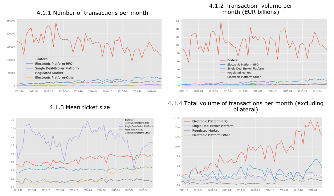
4.3 Recent studies of Electronic Trading
Following the crisis, large global banks reduced the size and changed the composition of their balance sheets. The sharp reduction in banks’ inventories of corporate bonds raised questions about whether they were committed to their traditional role in making markets in these securities.
In this context, some industry participants argued that the successes of electronic trading in equities could be repeated in the world of bonds. For example, Barton (2013), focussing particularly on government bonds, argued that participants were moving towards e-trading in fixed income because it could offer superior price discovery, more execution certainty, and post-trade transparency as well as smoother clearing, settlement and reporting (straight through processing-STP).
In 2013, McKinsey and Greenwich Associates published a widely cited study of electronic trading in corporate bonds. It was based on a survey of 117 US and European institutional investors plus interviews with sell-side dealers. The survey concluded that while some elements of electronics were influencing market practice, full-fledged e-trading in corporate bond markets would be slow to arrive. The report found that, at that time, most (perhaps 80%) of e-trading was conducted on multidealer Request-For-Quote (RFQ) platforms, and argued that this would likely continue for some time to come.
The McKinsey-Greenwich study identified two trends that tend to favour growth in electronic trading: smaller trade sizes and more frequent trading. These might result if dealers had less balance sheet capacity and, so, were reluctant to make markets in size. However, evolving market structure itself might contribute to these trends. In particular, in the US, the increased post-trade transparency introduced with TRACE could discourage dealers from taking large positions if they felt these could become known to their trading competitors. (See the discussion in Section 5 of this report).
The McKinsey-Greenwich report noted that strong growth in corporate bond issuance encouraged by the prevailing low interest rate environment created the impression of high trading volumes but that this was a cyclical phenomenon. There was no real evidence that the market structure was changing toward a more active secondary market for most corporate bonds. Indeed, the authors cited research by MarketAxess which showed that, in 2012, as much as 38 percent of US outstanding corporate bonds did not trade even once, 23 percent traded only a few times a year and, only 1 percent traded every day.
The study did point to a variety of initiatives aimed at integrating various pools of liquidity. These could represent ways in which technology could help support secondary trading of corporate bonds. The authors felt that all-to-all trading (A2A) might take hold, however, not in a continuous form but, more likely, through venues that offered periodic batch auctions.
A number of commentators on the McKinsey-Greenwich study emphasised the upside potential of electronic trading. For example, Markets Media (2013) quotes a credit trader as saying: “There are certainly lots of corporate bond issues that are liquid and have adequate trading volume where leveraging technology can make the trading process tremendously more efficient for investors. We know this because our estimate is that close to 50% of the daily corporate bond trades involve some sort of electronic connectivity”.
In 2014, ICMA published a study focussed specifically on developments in the market for European Investment Grade (IG) corporate bonds (see ICMA (2014)). This drew on interviews with corporate participants and included an assessment of the prospects for electronic trading. The ICMA study found that compared to the US, electronic trading in Europe had made greater inroads in the trading of corporate bonds. Specifically, electronic trading contributed to enhanced data management permitting participants better to identify holders or potential buyers of bonds.
The report found that three platforms appeared to be market leaders in Europe: Bloomberg, MarketAxess, and Tradeweb. Market participants they interviewed estimated that these three platforms accounted for more than 40% of the total number of transactions in IG credit. Expressed as a percentage of total market value, their share was likely much less because most of the trading on platforms was for small trade sizes as compared to the large trades that tended to go to the traditional OTC market. The report argued that it would be difficult for new platform entrants to mount a credible challenge to these three leaders in electronic trading or to the broker/dealers in the OTC market.
Subsequently, a number of new trading platforms have appeared. Some of these aim to encourage new participants to play a role in providing liquidity. For example, at least one has attempted to lure new sources of risk capital to the market by adopting rebates to respondents to RFQs in a manner similar to equity platforms which use a maker-taker pricing model.43 However, none has disproved the view expressed in the ICMA study that electronic trading would fail to rival the OTC market.
One international survey of fixed income electronic platforms predicts that most of the 33 electronic corporate bonds trading platforms operating in 2015 along with 8 new venues in the pipeline will have failed by 2018.44 The basic difficultly has been that none of the platforms has proved to be viable without the active involvement of the major dealers. The survey argues that the focus of innovation should not be to replace the broker/dealers but rather to increase trading efficiency so that greater trading volume can be supported using smaller dealer inventories of securities.
Some initiatives are attempting to put this principle into practice. For example, the Swiss exchange SIX has teamed up with Algomi which builds social networks for the corporate bond market. The hope is that improved networking can be put to use in facilitating large block trades. In essence, this activity aims to use networking to engineer the “double coincidence of wants.” MTS, the fixed income trading venue that is part of the London Stock Exchange group, is using a search engine provided by B2SCAN to allow investors to search for specific bonds or lists of bonds and then execute trades on the MTS platform.
4.4 Electronic trading of bonds in its various forms
The surveys of electronic trading in bond markets described in the last section suggest that electronics can support trading activities at various stages of the trading cycle from discovery of the market conditions including price, to trade negotiation and execution, and on to post-trade processing. Furthermore, details in the way that electronically supported trading actions operate can differ significantly across alternative platforms. So, what exactly do we mean by “electronic trading” and how can we describe the alternative forms that it takes?
Several recent studies have provided useful taxonomies of electronic trading. One broad-based effort was that of a working group of the BIS Market Committee published in January 2016.45 This survey covered international fixed income markets such as those in sovereign and corporate bonds and other fixed income cash instruments. The mandate of the BIS group covered large benchmark sovereign issues of the type that attracted high levels of trading activity before the advent of electronic trading. These instruments obviously differ from corporate bonds that are our focus here. The BIS Market Committee report characterises types of electronic trading and contrasts it with traditional OTC voice-trading using the graphical depiction displayed in Figure 4.2.
The traditional OTC market depicted on the left-hand-side of the figure is a network consisting of nodes that are either dealers, customers (clients), or brokers. The edges that connect dealers to customers or to other dealers are voice communications lines that have been established by pairs of participants who have established a trading relationship. There are effectively no branches connecting customers with other customers. All the trading relationships are on a bilateral basis.
In addition to direct trading between two dealers, the inter-dealer market may involve a broker that will arrange a trade for a dealer by searching among other dealers for an appropriate counter-party. During the broker’s search, the identities of the counterparties are not revealed (although, the broker would know the set of potential counterparties with whom the dealer has trading relationships). Once the trade is agreed, however, clearing and settlement proceed on a bi-lateral basis between the two dealers, i.e., the broker does not enter as principal in the trade. Thus, post-trade, the identities of the two counter-parties are revealed.46
The right hand side of Figure 4.2 depicts a variety of new trading mechanisms for bonds that have been introduced since the advent of electronic trading. Focussing first on the relationships between dealers and customers, on the extreme right there is a branch connecting one dealer with one customer in the traditional manner. In addition, there are now two possible electronic platforms that may intervene between customers and dealers.
An SDP is a single dealer platform. This is an electronic platform organised by a single dealer in which the latter can perform pre-trade discovery and trade negotiation electronically with its customers. Post-trade processing may also be provided as part of the same platform. The modalities of each stage can differ across platforms. They may also differ within a given platform depending on the trading relationship agreed between the dealer and the customer and, perhaps also, the option chosen by the customer.
The diagram depicts one branch running from the SDP to one customer. The SDP may be connected to multiple customers simultaneously, however. This would be true when a dealer posts firm bids and offers for a particular security to all its participating clients simultaneously. Alternatively, the dealer could hold a sealed bid auction by advertising a block of a security that it is offering for sale.
A more usual mode for corporate bonds would involve customers entering an RFQ (Request For Quotation) and the dealer posting its response through the SDP. The RFQ could be a two-way (bid and ask) or one-way only and the quotations supplied could be firm or indicative. The RFQ could be open to counter responses (price and/or quantity) by the client. By its nature, the identities of the dealer and the customer are known at every stage of the process. Note that in an SDP, dealers are not directly in competition with one another, although the client may be simultaneously negotiating with other dealers through different means.
One might ask: what is the difference and possible advantage of an SDP used with RFQs compared to a voice trading relationship? One possibility is that either the dealer’s actions (involving the SDP) or the customer’s or both could be more fully automated permitting algorithmic trading. In principle, this could be performed at very high speeds as occurs in equity markets. The episodes of very high, short-term volatility that have been observed in bond markets have been confined to the large issue, sovereign bonds.
On the face of it, the advantages of high speed trading would not appear to be as great for most corporate bonds. However, even with such bonds, however, the ability to automate processes could have cost and risk-reduction advantages. For example, if an Exchange Traded Fund (ETF) based on a corporate index needs to increase its holdings, executing this dynamically using an algorithm could have distinct advantages including increasing speed and reducing tracking error.[47]
An MDP is a multi-dealer platform. This is a platform organised to give access to trading by participating dealers and customers. MDPs share some of the features of SDPs as just described. The main difference is that an MDP opens up the possibility for direct competition among dealers for customer business in a single venue in which dealers are constrained by a common set of rules regulating activity on the platform.
47 As discussed in Section 7 of this report, bond ETFs have enjoyed strong growth in Europe as well as in the US.
This could make the discovery process more transparent. For example, customer initiated RFQs could be sent to a set of dealers who would have a limited time to respond. Responses may not be revealed to anyone until the response period has elapsed, at which time the customer could accept the most attractive quote (or quotes if several need to be hit in order to complete the desired trade size). In the terminology of market microstructure, this is a periodic, sealed-bid auction with reservation value. In Section 5, where transparency is discussed, we examine empirical work on a platform of this type that has been investigated using TRACE data in the US.
Platforms can operate within the inter-dealer market framework as indicated in the graphic. Again, a number of alternative trading protocols (RFQs, central limit order book (CLOB)[48], etc.) are possible. Also, information revelation may occur at different points in time. Some venues may be “lit” (in which case the identities of dealers making quotes or issuing RFQs are revealed at all times) or “dark” (in which identities are not revealed prior to trading and possibly may not be even after if the trades are cleared) or somewhere in-between.
The diagram includes a new category of players in the inter-dealer market. This is the principal trading firm, that is, a firm that puts its own risk capital at stake in making and taking liquidity in the market involving dealers. These could be hedge funds or other fund management firms that have the capital and expertise to trade in such markets but do not have direct access to the dealers’ traditional clients.
Finally, although this is not depicted in the graphic, a platform connecting multiple dealers and multiple customers could be developed. This is the A2A structure that some commentators imagine will ultimately come to replace the traditional bond market trading structure entirely. The fact that it is omitted from the graph reflects the fact that the BIS Markets Committee working group found the A2A did not account for a significant amount of bond trading at the time of their study.
Another observation of the BIS Markets study is that most dealer-to-client platforms in fixed income markets are based on the RFQ trading protocol. RFQ systems greatly in the degree to which (a) the quote requester or quote receiver reveals its identity, (b) the sign of the order (buy or sell) is revealed, (c) how many and what kind of participants may receive RFQs, and (d) how much quotes are executable or indicative.
On point (c), the study found that most such platforms allow customers to query only a limited number of dealers. The study identifies major RFQ systems: Tradeweb (majority owned by Thomson Reuters with ownership stakes by 11 banks that also participate on the platform), BondVision operated by MTS, and Bloomberg.
The final observation of the study is that less liquid sovereign bonds and corporate bonds generally do not trade using the CLOBs and do not employ much automated
(algorithmic) trading. The conclusion is that “…platforms are not the appropriate solution for all securities, particularly for illiquid securities for which the risks from information leakage are high. For these securities, there is still a role for bilateral dealer-client relationships.”
Also in 2016, ICMA released a report on the future of electronic trading in the European market.49 As in the BIS Markets Committee study, trading in both sovereign bonds and corporate bonds was discussed. The report was rather forward looking,
48 “CLOB”, the Central Limit Order Book, refers to a centralised database of limit orders attempting to sketch a variety of possible forms that electronic platforms might find success in the European bond market. It did not reach clear conclusions, however, about which form might prevail and did not give a detailed analysis of the recent evolution of the European bond market structure.
In a companion publication, however, ICMA provided a very useful summary of the characteristics of 23 trading platforms and 5 other platforms offering market discovery services but without offering trade execution.50 The study classifies platforms with respect to the characteristics shown in Table 4.1.
Type Single dealer to client, multiple dealer to client, dealer to dealer, client to client, all to all, other
Information structure Anonymous (matched principal trading), anonymous (name give-up), lit (disclosed), Anonymous and lit, N/A
Minimum size of trade
Securities Government bonds, corporate bonds, agencies, supra-nationals, covered bonds, HY, emerging markets, ABS, money market instruments, REPOs, other
Trade types Cash, spread, basis, others
Price discovery Sourcing, aggregating, N/A
Pre-trade practices Firm, indicative, bilateral negotiation, N/A
Post-trade and reporting Analytics, research, participant links, regulatory compliance
Regulatory status Regulated market, Multi-lateral trade facility, systematic internaliser, other Source: ICMA (April 2016b).
Most of these responses to the survey questions (i.e., categories) are self-explanatory. The possible responses under information structure refer to various practices commonly employed by brokers. In “name give-up”, a broker identifies pairs of counter-parties that have established trading relations including reciprocal credit or clearing. Such counterparties contract directly with each other. With “matched principal” trading, the broker enters into simultaneous purchase and sale transactions with customers. The broker is responsible for settlement. In this way, the broker can maintain post-trade anonymity of its clients.
The regulatory status refers to the categories of venues that have been established under MiFID 2. Multilateral trade facilities (MTF) are platforms where multiple dealers and/or other participants can interact and execute trades. A regulated market (RM) is, essentially, a type of multilateral trade facility that is regulated by a specific public authority. A systematic internaliser (SI) is a proprietary trading platform operated by a broker-dealer that is subject to European trade transparency regulations as set out in MiFID and MiFID 2. These are discussed in Section 5 of this report.
Type Multiple dealer to Multiple dealer to Multiple dealers client, all to all client to clients; all to all Information Anonymous and lit Lit (disclosed) Lit (disclosed) structure
Minimum size of None None None trade
Securities Government, Government, Governments, corporates, corporates, supra- agencies, agencies, supra- nationals, covered corporates, HY, nationals, covered bonds, HY, covered bonds, bonds, HY, emerging markets, repos emerging markets, MMI, Repos ABS
Trade types Cash, spread Cash, spread, other Cash
Price discovery Sourcing, Sourcing, Sourcing, aggregating aggregating aggregating
Pre-trade practices Firm, indicative, Firm, indicative Firm, indicative bilateral negotiation
Post-trade and Analytics, research, Analytics, Analytics reporting participants links participant links, regulatory compliance
Regulatory status MTF MTF MTF
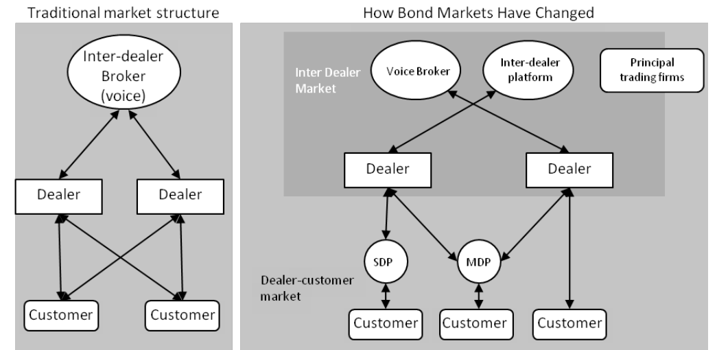
Note: The source is the BIS Markets Committee. MDP and SDP denote multi-dealer and single- dealer platforms respectively.
| Characteristic | Possible |
|---|---|
| Eligibility | Dealers, |
| investors, | |
| Method | Market |
| auction, |
| Platform | MarketAxess | Tradeweb | Bloomberg |
|---|---|---|---|
| Eligibility | Dealers, | Dealers, | Dealers, |
| institutional | institutional | Institutional | |
| investors, others | investors, others | Investors, | |
| others | |||
| Method | RFQ, other | RFQ, other | RFQ, other |
4.5 Results of platform interviews
As part of our study, we have conducted in-depth interviews with a selection of platforms which allow us to provide greater detail than that found in the ICMA mapping study and, also, to have a sense of how the platforms are evolving. We met with representatives of three of the main platforms that have been identified either in the BIS platform study or the ICMA 2014 and 2016 studies as having achieved a significant level of activity in trading of European corporate bonds: MarketAxess, Tradeweb and Bloomberg.
In each case, the interview included a detailed demonstration of their system’s features. One of the main purposes of these interviews is to provide greater clarity on the important issue of information structure. That is, we sought to ask: who among the participants on the platform knows what and when?
Table 4.2 presents a comparison of the three platforms according to the descriptors used in the ICMA 2016 mapping study. The entries for MarketAxess and TradeWeb are extracted from the ICMA study. Those for Bloomberg (which was omitted from the ICMA study) are our descriptions based on information we obtained in our interview or from Bloomberg publications.
According to this summary, the three platforms resemble each other. Our in-depth interviews confirmed that in some ways they are similar. In particular, the basic trading protocol that is at the heart of their systems and that accounts for most of their executed volume is an RFQ system. Furthermore, the systems have evolved out of traditional voice trading of the OTC market. Finally, for most of their business their platforms are interfaces between multiple dealers and clients who are mainly institutional fund managers.
However, our interviews revealed some significant differences in the way the protocols operate which affect the distribution of information among the various participants as the trading process evolves from pre-trade to trade/negotiation, and on to post-trade. Furthermore, comparing features that have been introduced in the last several years, further differences have emerged which suggest different views about how trading is likely to evolve in the future.
All three platforms can be viewed as growing out of the established dealer/client trading that has prevailed in the corporate bond trading in Europe (and to a large extent the US) for many years. On one side of the market are the dealer/brokers, typically the big banks that are the traditional providers of liquidity. On the other are institutional fund managers including insurance companies, mutual funds and ETF managers, hedge funds, and sovereign wealth funds.
These latter are the “clients” for the platform and they are the main sources of platform revenues either through platform subscriptions or commissions. Retail customers are not directly involved. The three platforms take the fragmented nature of the corporate bond market with its intermittent trading as a fact of life that is not likely to change dramatically any time soon.
At the heart of each of the platforms is an RFQ trading protocol which in its simplest form can be viewed as a periodic, batch auction with sealed responses (bids or offers) and undisclosed reservation prices. A client of the platform initiates a trading session by sending Requests for Quotations on a particular security to a list of dealers with which it has a trading relationship (trading is “enabled”), indicating the desired quantity and the direction of trade (client buys or client sells).
The dealers respond by sending their quote (both price and quantity) within the allotted time for the session. If the dealer is not interested, he may simply not respond. Once the client has received the responses, the winner is selected by the client. In principle, this is not necessarily the highest bid or the lowest offer. The client’s decision may also depend on the basis of the quantity in the response, the strength of the trading relationship, etc. In practice, in order to comply with best execution requirement imposed by MiFID, clients almost always do select best bids or offers.[51] However, if the client chooses, he may reject all the proposed trades.
For some of the basic parameters involved in this RFQ protocol, the three platforms have, until relatively recently, conformed to a sort of standard convention for RFQ systems in European credit markets. Trading sessions were limited to 3 minutes, but in practice trading was often much faster than that, perhaps 20 seconds or less. Clients could send RFQs to up to 6 dealers simultaneously. Dealers must be enabled, i.e., have established trading relationships with the client. Settlement arrangements (e.g. T+2 at a particular ICSD) are to be arranged bilaterally by the two principals to the trade. Responses to RFQs are meant to be firm quotes, i.e., executable if the response is accepted. However, the platform does not guarantee this and any failure to fulfil the conditions of the trade becomes an issue to be settled bilaterally between the two principals.
However, these conventions for RFQ systems are in the process of changing, and the three platforms are making changes to their protocols which introduce significant differences among them. These changes can be viewed as responses to pressures coming from the participants, in particular the fund managers that are the clients of the platforms. These clients have found that increasingly they are unable to execute desired trades following the basic protocol above. They find that even though they have an established trading relationship with a dealer, the dealer often will fail to respond to an RFQ.
The responsiveness of the dealers has, also, become more volatile. Sometimes a given dealer will respond only on one side of the market (only bids or only offers). Sometimes, it will be the other side. Thus, there has been an erosion of the sense of obligation to service a liquidity need of the client in order to maintain a reputation as good market maker. This reflects increasing P&L pressures on dealers in the face of increased costs (including regulatory capital charges). Dealers are tending to specialise in certain market segments. For example, regional banks may only deal in home-issued IG financials. These changes in dealer business models have meant that investors have a hard time predicting where to turn to fill their liquidity needs.
What have been the responses to these pressures? First, the platforms are allowing clients to send RFQs to more than 6 dealers. MarketAxess has removed limits altogether. Clients can send RFQs to any and all dealers with whom the client is enabled. In early 2017, Bloomberg increased the limit of RFQs from 6 to 9. Tradeweb has introduced FlexRFQ. This allows clients to contact additional counterparties within the same trading session by eliminating dealers whose responses they judge to be too poor. For example, suppose a client has requested from 5 dealers initially and 4 have responded (2 good and 2 bad). The client can eliminate the 2 bad and the nonresponse, and issue 3 new RFQs to 3 new dealers. Note that the total number of RFQs is the same. However, 8 dealers in total know that the client has a trading interest in the security.
The platforms have responded as well to the high trade failure rates in the way the negotiation unfolds. MarketAxess has maintained the executable trade requirement in their RFQ platform. Indeed, the quotes are “click to trade.” TradeWeb has gone in the other direction and allows for fairly elaborate negotiations implemented through the platform. Reponses to an initial request are price quotes and quantity proposals that may differ from the amount requested by the client. The client can then counter with a different proposed price and/or quantity. The dealer can counter this price and/or quantity. And so on.
Furthermore, if FlexRFQ has been enabled, the client can eliminate some of the current dealers from the process and insert new dealers in their place. These new dealers then can respond. Note, however, that the old dealers still in the trading session are informed that a switch of a stated number of dealers has occurred and they have the right to revise their outstanding quotes in light of this. In Bloomberg, given the responses to the initial RFQs, it is for the client to pick up the phone with the dealer or dealers of their choosing to pursue the negotiations bilaterally.
The other way that the platforms are responding to clients’ perceived problems in obtaining liquidity is by giving pre-trade information about where the liquidity is likely to be found. This involves a variety of sources of information about indicative quotes and dealer axes, that is, information about their inventories and to some extent their trading intentions. Given its traditional business model as a data aggregator, Bloomberg provides on its RFQ platform a list of indicative quotes from a variety of sources.
These include regional exchanges where a security is listed and indicative quotes from dealers who are broadcasting a trading interest indicating prices and quantities on either or both sides of the market. They also include composite quotes such as BVAL that are computed by Bloomberg according to a proprietary algorithm. They include indicative quotes from banks with whom the client is enabled. Not all banks displaying an axe to a client are necessarily enabled for electronic trading. If so, the client can request such access through an RFE. If accepted by the bank, the client can include this bank in its RFQ.
TradeWeb has also invested a lot of effort into providing pre-trade information. They show to a client indicative quotes from client-enabled dealers. They also show a TradeWeb composite quote. This is based on results from Sweep which is a twice weekly dark pool (anonymous) among participating dealers for odd lot trading[52] of cash credits. This was developed in response to dealer needs because they were finding that in servicing ETF creation they had assorted small holdings clogging up their portfolios. They wanted some means of consolidation. Sweep has been very successful. The TradeWeb composite quotes are the trimmed mean bid and trimmed mean ask in the Sweep session.
In addition to these indicative prices, clients can see axes of enabled dealers. Dealers supply one of three possible tiered axes. Any given client will see the axes for any given security according to the tier to which that the client belongs. That is, for a given security the dealer will show some inventory information in tier A that will be seen by some clients. The dealer will then show other possibly different information for tier B for other clients, and similarly for tier C. Then, the dealer will determine
52 “Odd lot” is a stock order comprised of less than one hundred shares of stock whether a given client will see A, B, or C. In practice, therefore, important fund managers tend to see good axe information. Hedge funds and banks, who are viewed as more aggressively opportunistic, will not see as much. But, this is case by case and depends on market conditions and the particular position of the dealer at the time.
It is useful to recap the information distribution at various stages of the trading process from the point of view of the various players in the current RFQ platforms. This is given in Table 4.3.
Note that the way information is distributed on the system can shape the decisions made by various participants. In particular, informing the winning dealer about the 2nd best quote, gives some information about the degree to which he or she may have suffered from “winner’s curse”[53]. This information may prove useful in the future and, therefore, helps to incentivise dealer efforts in providing liquidity.
These are the main features of the RFQ platforms that account for most of the European corporate bond trade volume on the three sites. Each of the three sites has been developing ways of allowing traditional fund managers to begin to make liquidity as well as to take it. These are the All to All platforms (A2A) that are at various stages of development. TradeWeb’s approach to A2A is to allow clients to search among other participating clients’ RFQ flow to try to identify complementary trading interests. Even though they have introduced a dark venue for their interdealer, odd-lot trading system, Sweep, up to now they have not provided dark pool access to their clients.
of RFQ for a given of RFQ for a given of RFQ for a given security. Dealer also security. Dealer also security. sees the number of sees number of RFQs Subsequently, RFQs sent but not sent but not the negotiations take identities of other identities of other place bilaterally over dealers. dealers. the phone. Each Finally, client sees Client sees all dealer sees only the price quotes sent as responses (prices and history of their responses from all quantities) from all negotiation with the dealers. These are dealers. client. The client sees click to trade. Client and dealers all the negotiation then interact with histories. counter-offers. Client sees all negotiation histories. Dealer sees their own negotiation history with the client. Also, under FlexRFQ a dealer also sees if they have been dismissed from the negotiation or if a number of other dealers have been dismissed and replaced by new dealers. Dealer still does not see the identity of any of the other dealers involved.
Once the trade is The winning dealer The winning dealer The winning dealer concluded sees he or she is the sees he or she is the sees he or she is the winner and thus the winner and thus the winner and thus the price and quantity. price, quantity. The price, quantity. The winner also sees winner also sees the The 2nd best dealer the “cover” i.e., the “cover” i.e., the price sees that he or she price of the 2nd best of the 2nd best dealer. was 2nd best but not dealer. The 2nd best dealer the price of the The unsuccessful sees that he or she successful dealer. The dealer only sees that was 2nd best but not other dealers who had they were the price of the responded see that unsuccessful. successful dealer. the trade was done The other dealers who and that they were had responded see unsuccessful. that the trade was done and that they were unsuccessful. A non-responder does not learn anything about the outcome of the trading session.
MarketAxess introduced an A2A platform called Open Trading for European corporates in February 2015. This is part of their response to client discontent with service in traditional relationships with broker/dealers. In Open Trading, anybody can ask for liquidity. The client chooses a list to send RFQs. In most cases, they simply ask for the “market list”, i.e., the whole Open Trading world in the product segment. This request will be filtered through the platform so that a participant will only see the RFQs for products that are of interest to them. Responses are anonymous. There is a three-minute window that operates for standard RFQs.
In typical usage, a participant will send an RFQ through the traditional platform and also one through the Open Trading platform. The responses come back on a common screen with Open Trading appearing anonymously and dealer identities showing from traditional RFQ. MarketAxess maintains anonymity by taking the other side of each trade. They control the resulting operational risk by requiring all participants to have appropriate accounts with custodians that settle through the ICSDs. One advantage of this approach is that it simplifies the compliance with know-your-customer (KYC) obligations. A participant just needs to know MarketAxess rather than a potentially large number of counter-parties they might encounter on a non-anonymous A2A platform.
Finally, Bloomberg has introduced A2A in European corporates via a joint venture with State Street Bank. All trades are executed at State Street Global Markets, a subsidiary of State Street Bank.
All three providers report that A2A seems to be slow to take off and point to the same crucial obstacle: the difficulty of developing among institutional investors a willingness to engage in price formation. In part, it is a question of culture. Fund managers have not done this in the past. However, it is more a matter of cost. Making a price to provide liquidity requires traders and infrastructure. These require costly investments. Entering this business without an established market for the service is very risky. Many of the managers simply do not have the scale, scope and capital to take this on.
| Platform | MarketAxess | Tradeweb | Bloomberg | ||
|---|---|---|---|---|---|
| Pre-trade | Client sees indicative | Client sees | indicative | Client sees | indicative |
| quotes. | quotes from | dealers | quotes from | ||
| and composite | exchanges, | dealers | |||
| Tradeweb | quotes. | broadcasting | trading | ||
| Client sees | one of | interest, enabled | |||
| three possible | axes | dealers, other | dealers | ||
| from enabled | dealers | that potentially | could | ||
| with tier | determined | be enabled, | and | ||
| by the dealer. | Bloomberg | composite | |||
| quotes using | several | ||||
| algorithms. | |||||
| Bloomberg | gives some | ||||
| indication | (colour- | ||||
| coded) of | quotes that | ||||
| will be close | to | ||||
| executable | based on | ||||
| monitored | response | ||||
| record of the | dealer. | ||||
| The client sees | axes | ||||
| provided by | some | ||||
| dealers. | |||||
| During trade | Initially, client sees | Initially, | client sees | Initially, client | sees |
| negotiation | identities of all dealers | identities of | all dealers | identities of | all dealers |
| receiving RFQs. | receiving | RFQs. | receiving RFQs. | ||
| Next, dealer sees | Next, dealer | sees | Next, dealer | sees | |
| identity of requester, | identity of | requester, | identity of | requester, | |
| direction and amount | direction | and amount | direction and | amount | |
| 53 “Winner’s curse” refers | to the tendency for | the winning | bid in an | auction to | exceed the |
| intrinsic value of the item | purchased |
4.6 Pre-trade market discovery
In the preceding sub-section, we observed that to varying degrees the established electronic trading platforms have been developing their own tools to provide market participants with enhanced capability to locate pools of liquidity in which others with a complementary trading interest are present. Several firms have now specialized in developing electronic pre-trade market discovery tools that can be integrated into a trading platform or can be used, on a stand-alone basis, as a support for trading via traditional voice-based markets.[54]
Algomi, B2SCAN and Project Neptune are three firms that attempt to create a framework in which participants give access to trade-relevant information in exchange for gaining information useful for their own trading objectives. They, then, attempt to aggregate information intelligently to shed light on which market participants (either dealers or investors) may be open to trading and in what amounts.
The fundamental problem in trading corporate bonds which reflects the market’s inherent tendency toward fragmentation is that at any given time a large fraction of the bond inventory is in the hands of the buy side. The broker/dealers who channel trading activity do not hold a significant fraction of the overall bond inventory in their trading books. Their main asset in market making is their informational advantage which comes from their network of trading contacts and from the observation of recent trade flows. In this context all agents are strategic. On the one hand, all agents are hungry for information about where securities are held or sought. On the other, no agent is willing to reveal their trading interests unless it is necessary to achieve their trading objective.
The pre-trade market discovery platforms are all grappling with the same problem: how to elicit information about the trading intentions of participants who fear that in signalling their trading needs they will leave themselves open to exploitation by other traders. The aim is to overcome this fear and to guide market participants towards mutually beneficial trading opportunities whereby fair bargains can be struck. They are approaching this problem in different ways reflecting their particular business networks, different histories, and different conceptions of the technology. At this stage, no single approach appears to be the dominant strategy. However, there are signs that overall they are helping to promote a change in trading culture and market microstructure that could reshape trading in profound ways.
In preparing this report, we met with principals in each of the three leading pre-trade data aggregators in the European corporate bond market. Comparing the differences and similarities of their business models gives some useful insights into the challenges of balancing the interests of the diverse stakeholders in this market segment.
B2SCAN was established in 2011 to provide trade information aggregation in European corporate bonds. The basic model is that large dealers supply their trading axes, that is, their firm indications to deal securities on a daily basis. B2SCAN integrates all this information as well as keeping track of counter-parties with whom dealers maintain trading relations. Dealers provide lists of counterparties with whom B2SCAN can display axes.
Participants initiate a query by specifying a variety of search criteria: country of issue, currency, industry segment, issue size and so forth. The platform then displays the securities satisfying these criteria indicating ISIN and number of axes. There is a fuzzy search functionality that can be used to search for bonds that share the characteristics of the bond for which an inquiry was made and for which there may be compatible trading interest available.[55]
The key to the success of the business model is building participants’ confidence in the idea that by giving a little they stand a good chance of getting something of value in return. For the dealers, it is important to know that if they provide some information about their trading interests, they can control the types of clients who will see those interests. Furthermore, by being among other reputable dealers on the information platform, they will naturally attract comparably serious, real money investors to the site. And in any event, they can filter the clients they are willing to deal with. For the clients, it is important to have the confidence that the information displayed is accurate and that dealers’ expressions of trading interest are genuine. For all concerned, the desired end result is a higher rate of successful trading.
Starting with HSBC, Bank of America Merrill Lynch and Citi, B2SCAN has built up the participation of a significant number of the major dealer banks. On the buy side, the client base developed strongly in the French and Nordic segments. In 2015, the B2SCAN platform established a link-up with the trading platform MTS as part of a joint venture with London Stock Exchange. The B2SCAN platform could, potentially, be integrated into other trading platforms. Consequently, future link-ups with other platforms might be a way forward. For now, it is based on the traditional dealer to client model and has not actively sought an outlet into A2A.
55 These algorithms are based on fuzzy set theory that employs a hierarchy of characteristics which allows degrees of association to be established even when information on characteristics is incomplete.
Set up in 2012, Algomi (like B2SCAN) reflects its principals’ earlier experience in bond trading at a major dealing bank. This involved the development of one of the first dealer bank internal trading platforms in the early 2000’s. After further work in the context of dealer proprietary platforms, the idea came to take some of the lessons to tackle the problems of pre-trade market discovery into a more open environment.
Algomi’s first tool, called ‘Syncronicity’, is aimed at broker/dealers. It attempts to collect all the information that passes through their trading systems including executed trades, voice expressions of trading interest, RFQs, and axes. These are aggregated into a form that can be correlated with the trading queries coming from clients or other dealers.
Algomi introduced a second tool called ‘Honeycomb’ in 2015 which is directed at the buy-side. Using the data feed collected by participating dealers, it characterises each dealer’s involvement in a security in a way that allows the client to assess the likelihood of hitting upon a good trading prospect. Specifically, the clients are provided information about enabled dealers’ axes. They also receive softer information or “colour” such as information that the dealer traded the same bond recently which may suggest the dealer may be able to identify other parties with a compatible trading interest even if the dealer itself does not have the bond in its axe.
Up to this stage of a client’s enquiry, the identities of the dealers in the honeycomb cells and the identity of the party making the enquiry have not been mutually revealed. However, when the enquirer clicks on the honeycomb cell, the identity of the dealer is revealed to the enquirer and the dealer is informed that the enquiry is underway and of the identity of the enquirer. From that point onward, the two potential counterparties can carry on a negotiation by messaging or by voice as they like.
The system is designed to provide a buy-side client with an informed basis for selecting a single potential counterparty with the highest probability to make a mutually beneficial trade. In conception, it is a totally different approach to the idea of sending out RFQ’s to a wide list of potential counter-parties. The aim is to minimize the chances of information leakage as it pertains to this specific trade. It does not aim at building up a long-term business relationship, although, that can be an outcome as well. Rather, Algomi is trying to unlock the potential to capitalize on potential trading opportunities that come and go in the market place.
Furthermore, by reducing risks of information leakage, Algomi aims to promote the capacity of large size trades. Again, this is the opposite of the alternative approach which uses a combination of trades through RFQ platforms plus approaches to brokers plus approaches to dealers directly as part mixed-strategy for working a large order into a number of smaller clips.
Algomi has the participation of about a dozen large dealer banks which feed axes into the Algomi system. On the client side of Algomi’s ‘Honeycomb’ there are 100 or so buy-side firms actively engaged. While the product has developed as a tool to support a network of traditional dealers as they face buy-side clients, it has the potential for aiding the buy-side firms to evolve toward becoming active makers of liquidity. In this sense, it may be a step along the way to spreading A2A in the corporate bond space.
Project Neptune is, also, the brain-child of ex-sell side bond traders. Project Neptune is a data aggregator. It is attempting to let the platform do more of the trading process electronically. Specifically, the aim is to combine more detailed information about the bond characteristics (”the whole term sheet”) which is often only communicated in abbreviated form on most platforms or data aggregators. This is combined with information about axes and inventories.
As with B2SCAN and Algomi the success of the business model rests on the ability to pool information from the major dealers who collectively have the best information about where the bonds are and where there might be an inclination to trade. This can be used to guide investors to the dealer who, if approached, is most likely to produce a successful trading outcome that is, moving the whole amount to be traded at a good overall price.
Project Neptune’s design differs, however, in that it attempts to formulate search at a higher level than an individual ISIN and in so doing does not prematurely exclude some possible market niches which may provide the best trading opportunities. Furthermore, after stating the search objectives in terms of high level characteristics, the platform itself carries out the analysis to narrow down the search to the best prospects. At Project Neptune they refer to this as “genuine electronic trading” rather than mere automation of one mechanical step in the trading process. This is involves a genuine optimization rather than displaying exhaustively the results of a fuzzy search. In this way, the platform is meant to provide “street positioning for the buyside”.
The aim of Project Neptune is to have axes provided in real time from the whole market. Currently, they have all the dealers that they consider to be “tier 1” on their board as principals in the company and a number of the second tier dealers and major buy-side players as well. According to their website they have over 17,000 real time axes covering more than 10,000 different bonds for a gross notional of more than $100 billion. Neptune is designed as an open standard network offering clients considerable flexibility as to how to access the information including in-house order management systems, third party systems and Neptune’s own desktop.
Project Neptune is still at a relatively formative stage, and it remains to be seen if its design gains wide acceptance, in particular on the buy-side. Its approach is based on the premise that the buy-side is interested in being relieved of some of the heavy tasks of sorting through huge quantities of disparate information in order to home-in on pockets of liquidity in areas of their trading interest.
One obstacle they face is overcoming a natural initial scepticism about how the buyside and sell-side interests are being balanced in the platform’s optimization that homes in on a proposed trading sweet-spot that corresponds to the client’s initial highlevel query. Of course, it would be nice to have the computer do some of the heavy lifting in bond trading. But, they may feel insecure leaving this to a “black box” that they only vaguely understand.
5. Transparency and Liquidity
Summary of findings:
1. We examine the issues of pre- and post-trade transparency. We note that the traditional OTC voice market has low transparency in both respects. This may be in the process of changing under the influence of new regulations and the evolution in market microstructure (including electronic trading).
2. The best source of information on this is the experience of US markets in which TRACE was introduced in 2002. We review the literature on this occurrence in some detail. TRACE introduced post-trade transparency to US markets, but not pre-trade transparency. There are indications that this led to lower trading costs for more liquid issues. However, there is also evidence that this has reduced trading frequency for other issues that are naturally less liquid (e.g., because they are lower rated).
3. We discuss the European experience. Electronic platforms have made inroads by introducing some additional transparency pre-trade in the sense that RFQ platforms facilitate the use of batch auctions.
4. MiFID II will potentially affect markets significantly. The pre-trade transparency regime could bring about major changes in market structure if it is extended to relatively less liquid securities by inducing dealers to retreat from making markets in some market segments.
5. If pre-trade transparency is limited to a very small number of clearly liquid benchmark issues, then the major impact will be felt through post-trade transparency. There, the effect will be to give coarse, but timely, information to the market which will help identify pockets of potential trading interest and to provide a price anchor that will facilitate negotiation. This could facilitate greater use of RFQs and other methods and, ultimately, lower effective trading costs.
5.1 Introduction
This section addresses question 3 of the Introduction, namely: what is the importance of pre-trade and post-trade transparency obligations for efficient price formation for different types of corporate bond and what are the implications for trading behaviour and liquidity?
MiFID 2 (adopted by the EU in 2014) mandates a pre-trade and a post-trade transparency regime somewhat analogous to the regime that was introduced for equities by MiFID 1 in 2007. At this stage, the Level 1 and Level 2 elements of implementation have been agreed and will come into effect in 2018.56
Since the major changes to the transparency regime in Europe have not yet occurred, we cannot directly answer the question posed through an econometric analysis of historical measure of liquidity before and after the liquidity regime changes. In the US, a major change to the transparency regime for corporate bonds was mandated by regulatory changes in the early 2000’s, and implemented with the Trade Reporting and Compliance Engine (TRACE) starting in 2002.
The information produced by TRACE has been subjected to extensive analysis by regulators, academics and finance practitioners. This is by far the richest source of information on the effect of transparency on liquidity in a fixed income market. However, it reflects the structure of US corporate bond markets which may differ from European corporate bond markets in some respects.
In this section, we explore the current state of transparency in the European corporate bond market and attempt to understand the likely effect that the introduction of the MiFID 2 transparency regime will have on the liquidity of this market both in the near term and in the long-run after market participants have been able to adjust.
In order to do this, we first examine the conclusions of studies of the transparency regime in US markets, taking into account details of the micro-structure that have been identified as important in determining liquidity outcomes. We, then, discuss the current state of transparency in the European corporate bond market, again, taking care to identify the important micro-structural characteristics of that market. From this, we assess the degree to which lessons from the US experience with transparency in corporate bond trading are likely to be reflected in MiFID 2 implementation.
Our findings are as follows. Based on the current plans for MiFID 2 implementation, we anticipate that, initially, the major effect of the new pre-trade transparency regime will be felt by a relatively small number of comparatively liquid corporate bonds. For these bonds, based on the predictions of theory as well as practitioner experience, it can be expected that liquidity, as measured by frequency of trades, may drop off as trading gravitates towards forms of negotiation for which issues of information leakage may be less severe.
If, subsequently, the criterion for a liquid market is phased in as planned, these same pressures could be felt by a significantly larger number of bonds. If so, this could be a major driver of change in the microstructure of the market. During the initial phase, most bonds will be considered illiquid, and, for these bonds, the main effect of the new reporting regime will be felt through the post-trade publication obligation.
This is on the assumption that details of price and quantity of individual transactions will be disseminated widely enough to be usable by all institutional participants in the market within about 48 to 72 hours of a transaction occurring. This will provide rather coarse information with a significant delay, but it will still be a significant increase in the degree of post-trade transparency of the market compared to the situation that has prevailed in the European corporate bond market up until now.
for bonds has been revised. The current intention is that the standard be phased over four steps. The first will coincide with the year in which MiFID 2 comes into effect (2018). This willbe revised progressively until the fourth step is reached. Each year, ESMA will submit a new RTS adjusting the transparency regime to next step, unless ESMA concludes that a move to the next step in not warranted. The plan for criterion (b) is 15 trades per day in the first stage followed by 10, 7, and finally 2 trades. However, it is anticipated that these standards will be reviewed in light of market experience. See, European Commission (2016a) and, especially, (2016b) Table 2.1, p. 13.
Such transparency will enable institutional investors and their data providers to better identify bonds that are likely to be in the hands of broker/dealers and other active market participants who may be receptive to a request for quotes. It will, also, provide an important point of reference, serving to anchor the price discovery process for the market as a whole. This could, potentially, stimulate greater use of batch auction trading mechanisms and, therefore, indirectly induce a greater degree of pretrade transparency as well.
5.2 What is a transparent market?
The transparency obligation mandated by MiFID and MiFID II and by other regulatory initiatives is motivated by the idea that the public interest is best served if trading takes place in an open and competitive market. This principle is very intuitive: if the market is open and transparent, participants will all have equal opportunity to pursue their own interests.
The same principle of market fairness also underlies the closely related regulatory initiative to impose a best execution obligation. That is, when investors participate in markets only through the offices of agents engaged to work on their behalf, then, those agents should be obliged to provide investors with the best available execution of their trades.
These general principles have been studied in detail by economists.[57] The classic work in this area is Walras’ analysis of the competitive auction market. The Walrasian market is a centralized market for a homogenous product that is pre-trade transparent. This transparency follows because everyone who wants to trade given goods knows where to go, can inspect the goods to verify their quality, and, then, can observe the price that is determined in an open auction.
Classical economics did not concern itself with post-trade transparency because it did not consider (nor did it have the tools to deal with) goods that are durable (or storable). This complication has only been seriously studied recently, as will be discussed below.
5.3 Transparency and the structure of the corporate bond market
In the early part of the twentieth century in some European countries, corporate bonds were a major source of funding for firms. Furthermore, they were traded on national exchanges in a manner similar to trading of equities and, in this way, achieved a relatively high degree of pre-trade transparency. However, this was transparency in a very local market where communication took place at a pace not at all comparable to today’s markets.[58]
Subsequently, the corporate bond market, both in Europe and the US, gravitated toward a principal-based, over-the-counter (OTC) market form, in which dealers make markets in bonds by quoting prices.59 Typically, dealers maintain inventories in the bonds that they sell, and often their inventories are acquired through participation as an underwriter in the original (primary) issue. A client (typically, an institutional investor such as an insurance company or pension fund) may request a two-way, firm quote for specified quantity. More frequently, the client will indicate both the quantity and direction (buy or sell) of the intended transaction. Once agreed, the trade is completed with the dealer entering as a principal.
From that point, the dealer is at risk and will generally attempt to lay-off his or her risk in the inter-dealer market. If the dealer enters the client trade as a buyer, then he or she will sell down their position to restore their holding to the desired level of inventory. If the dealer has sold bonds to the client, he or she will buy on the interdealer market to restore inventories to target levels. In some cases, the dealer may have sold short in the sense that his or her inventory of the bond at the time of the client trade is insufficient to cover the amount sold. In this case, the dealer will be under pressure to source the bonds in the inter-dealer market in order to meet the agreed settlement date of the client trade.
Alternatively, the dealer can cover the short-sale temporarily by sourcing the bond by entering a reverse repurchase agreement. However, if the dealer needs a specific issue, this may involve a “special,” that is, a transaction in which the dealer provides funds requesting the counter-party to post a specific bond as collateral. In this case, the dealer may be obliged to make a concession by lowering the repo rate.60
If a client requests a quote that would be very difficult to cover in the inter-dealer market in a short time period (relative to the underlying volatility of the bond value), the market-maker may feel that the trade is too risky to perform as a principal. In that case, they may agree to proceed on an agency basis and attempt to arrange a matched, back-to-back set of transactions, or simply to serve as a broker. This flexibility in arranging transactions is the basis of referring to major market makers in the OTC bond market as broker-dealers. As described here, the OTC market for corporate bonds departs significantly from the competitive Walrasian auction market.
• It is fragmented rather than centralized: to learn the price, investors need to search among alternative dealers to find those willing to transact in a particular bond.
• The products to be exchanged are not homogeneous: investors may be looking for a bond with certain characteristics and the dealers may propose a number of possible bonds that approximately meet those characteristics and can be sourced in the market.
• It is not pre-trade transparent: in advance of searching, the available prices are difficult to know. Also, it is difficult to carry out multiple searches so as to achieve comparability of quotes.
• Furthermore, the corporate bond market is not post-trade transparent: in the pure OTC market, trades are meant to remain confidential for the two counter-parties involved.
• One could almost say that the pure OTC corporate bond market is a prime example of the “fully opaque market.” This has led some analysts to conclude that it would be hard to imagine that pre-trade transparency could work in the corporate bond market based on bilateral negotiation market structure.61
• Furthermore, in an OTC market relationships can matter. Investors will build up relationships with their dealers just as clients build up relationships with their banks through repeated interactions so that building up a reputation for reliability and fairdealing can be highly valued.
Does this mean that the opaque market structure of OTC corporate bond trading is inefficient? Not necessarily. It may be “second best” efficient in the sense that it is efficient within a class of market structures that are constrained by certain market imperfections.
Over the last ten years, several theoretical contributions have clarified the foundations of OTC trading. Most of this literature has looked at the implications of alternative market structures when market participants possess different information about the factors affecting the value of a financial instrument.62
In the context of corporate bonds where (i) value depends upon the likelihood that a firm will default and (ii) the value of firm assets in case of default and the costs of bankruptcy are very hard to estimate, the assumption that investors are differentially informed is very plausible.
Recently, Babus and Hu have studied the determinants of asset market fragmentation when investors have heterogeneous valuations for a traded asset.63 Investors can either trade with other investors on a one shot basis (in which case they protect against counterparty risk by demanding collateral) or, alternatively, they can trade through intermediaries repeatedly on an unsecured basis. Babus and Hu find that in some circumstances market fragmentation is an equilibrium outcome. Furthermore, fragmented market structures exhibit greater trading volumes and can result in allocations that are Pareto superior to centralized markets operating under the same information constraints.[64]
These theoretical contributions may help to explain why OTC trading has come to be the predominant market form for corporate bonds. It would be wrong to conclude, however, that OTC trading is the only form of trading that is sustainable. In fact, retail trades of small size are typically handled by intermediaries crossing client trades internally with any imbalances being absorbed by their inventories. In addition, some trading activity has continued on exchanges.
However, a serious challenge to the OTC market for large scale, fixed income trading has appeared only over the last 15 years or so and has been driven by two factors: technical change and new regulations. The consequences of these two forces are most evident in equity markets where trading has been dramatically reshaped with the rapid growth of new trading platforms and the introduction of electronic trading. The latter has increasingly reduced the role of stock-exchange-floor-based market-makers, and has given rise to high-frequency trading. Some analysts have argued that similar developments should be expected for bond and other security markets. Thus, it is useful to review briefly some of the major developments that have taken place in equity market structure.
5.4 How regulation and technology changed equity market structure
In the US, the Alternative Trading Systems Regulation of 2000 disrupted the position of traditional stock markets by opening up trading to new entrants, mainly using electronic platforms. The second major regulatory change in the US was the introduction of the National Market Systems Regulation in 2007 which established rules of access and priority across multiple venues (see O’Hara (2015)).
These changes set in motion a collective rethink of how to approach the buying and selling of equities. This has given rise to a totally changed market structure and forced a reassessment of traditional notions of an efficient market. All players have become strategic in their outlook. This includes investors, intermediaries, and the platforms themselves. Some of the trading venues operate electronic limit orders books (LOB), formerly viewed as the epitome of pre-trade transparency. However, these co-exist with traditional floor-based specialists, internal crossing networks, and dark-pools all operating with different rules of access and communications protocols.
The result has been an extreme fragmentation of the trading environment. Has this improved liquidity? Quite possibly. Has this improved pre-trade transparency? Locally, yes (that is, in some specific venues) but globally, no. In this regime, agents must search pro-actively for liquidity across multiple venues. The law of one price does not hold generally and there are arbitrage possibilities to be exploited. However, in pursuing them, speed is essential. Dark trading becomes important for players for which size of trade would place them at a strategic disadvantage in a very transparent setting. Instead of trading through large orders that could compromise the position of your counterparty, large orders are worked across multiple venues. Average trade sizes have dropped generally.
It might be thought that these developments have disadvantaged small traders, but this is not necessarily the case. Retail trades are either crossed internally by an intermediary or obtain bulk trading rates through broker-dealers. These latter negotiate deals with exchanges who pay for order flow (because retail is not viewed as trading on information).
In Europe, there have been a parallel set of regulatory initiatives that have changed the environment for the trading of equities. The move toward financial market integration has been important in promoting greater competition by removing the barriers to cross-border financial transactions within the EU. With the full implementation of T2-S (Target 2- securities) in 2017, Europe will have stream-lined its post-trade settlement process and promises to significantly reduce costs of crossborder trades.
The main initiative affecting equities was the Market in Financial Instruments Directive (MiFID) which came into force for equities in 2007. At the same time, the technical developments that gave rise to new equity platforms in the US have generated similar developments in Europe. The result has, again, been a fragmentation of the market structure for equity trading and a strong growth of E-trading. It has been estimated that E-trading accounts for about 70-80% of cash equities trading (see McKinsey and Greenwich Associates (2013)).
One thing to note from this short summary of developments in cash equities trading is the importance of the details of microstructure. While early analyses argued that dark trading was negative for retail equity investors, the current thinking is rather that small investors have been the net beneficiaries of the evolution of cash equity market structure (O’Hara (2015)).
The reason for this lies in an important detail in the new environment which permits trading for order flow. Thus, Charles Schwaab, the big retail-oriented brokerage firm, is able to negotiate with a large broker-dealer a rebate for processing this flow business (after internal netting). This rebate can, in turn, be passed on to retail clients through lower commissions and trading price realisations closer to those realised by the large block trades of institutional investors. Schwaab is able to negotiate this rebate because retail flow business is viewed as very attractive in a trading environment populated by informed and uninformed traders since retail traders are likely to be in the latter category.
Details of the pricing protocol are also important in understanding the impact of venues that operate electronic limit order books.[65] In this context, agents that place limit orders to buy and/or to sell are viewed as “making liquidity.” Agents that hit the limit orders by making a market order “take liquidity.” Many venues adjust their pricing algorithm to incentivise the provision of liquidity. In the “maker-taker” pricing mode, the venue pays a rebate to agents that place limit orders and charges agents to place market orders. This has incentivised particularly the entry of HFT to provide liquidity because they have a comparative advantage in removing limit orders if the arrival of informative trading has been detected. Many HFT have made good profits from rebate flow in providing liquidity.
In Europe, MiFID as introduced in 2007 not only removed obstacles to entry for alternative trading venues for equity trading. It also established a pre-trade and posttrade transparency obligation for cash equity trading. The evolving structure of the European market has been characterised by a sharp fall in the average trade size and increased fragmentation of trading across multiple venues including internal crossing, dark pools and traditional exchanges.[66]
5.5 Regulation, technology and corporate bond market structure
We now turn to corporate bonds, our main area of interest. What are the implications of technological change and regulatory initiatives for the openness and transparency of the corporate bond market? And what is the effect of this for trading costs and other measures of market liquidity?
The first thing to note is some inherent differences between cash equities and bonds. In cash equities, the main financial contract issued by a given firm is common stock. In contrast, the corporate bond market has an inherent tendency toward fragmentation even of the primary market. Corporations issue bonds of various maturities and other terms and conditions (such as varying seniority status, amortization schedules and including options of various sorts) at irregular intervals. This pattern of issuance is driven in large part by the redemption schedule of maturing bonds and by the desire to match expected timing of cash flows of new investment projects being undertaken.
The net result is that for a given issuer (a specific legal entity) may have a large number of bonds outstanding at a point in time. Furthermore, the same corporate group may issue different bonds through different legal entities that make up the group.
Thus, overall the bonds of a given issuer group can be highly heterogeneous because may differ in many different quality dimensions which make value comparisons across bonds a complicated matter. It is this difference between a homogenous financial contract and a heterogeneous one that has led to the maxim “bonds are sold and stocks are bought.”67 That is, investors rely on sell-side institutional sales people to sort through all of the details of terms and conditions of various bonds to find suitable issues. In contrast, investors have an easier time in selecting stocks based on their analysis of the company, sector and overall market trends.
Nevertheless, as discussed in Section 4 of this report, changing digital technology and regulatory initiatives have changed some aspects of the corporate bond trading environment. The pressures for change have been strengthened by changed regulatory capital charges plus other changes to banking prudential regulations which are creating incentives for traditional dealer-brokers to reduce inventories and to retreat from the principal based liquidity provision.
5.6 Transparency in the US corporate bond market-TRACE
In the US, the main regulatory initiative that was directed at corporate bonds was the decision to impose a post-trade transparency obligation introduced by the SEC for most categories of corporate bonds. This has been implemented by FINRA (Financial Industry Regulatory Authority), the government sponsored self-regulatory body with representation from a wide range of securities markets stakeholders.
The transparency obligation is fulfilled through the Trade Reporting and Compliance Engine (TRACE), which began operations in July 2002 and which requires public dissemination (with some delay) of post‐trade price and volume information for corporate bonds. TRACE was implemented in phases, with actively traded, Investment Grade (IG) bonds becoming transparent before thinly traded, High Yield (HY) bonds. The TRACE initiative was an important experiment in mechanism design and, because it produces public information, gave rise to a series of academic studies analysing the effects of transparency on market liquidity and other pricing characteristics. These academic studies have the considerable benefit of being subject to third-party verification and public scrutiny, something that is sorely missing with respect to regulatory studies based on information that is restricted to regulators themselves by law or by regulatory practice.
The early studies of TRACE data were based on the first wave of bonds subjected to the transparency obligation, namely, the large-sized IG issues. By and large these studies find that, following the introduction of the dissemination obligation, trading costs on these issues declined as compared to bonds not subject to the transparency obligations.68 Edwards, Harris and Piwowar (2004) estimate that this increase in transparency reduced the bid-ask spread by about 5 to 10 cents (for a nominal par value of $100.) Goldstein, Hotchkiss and Sirri (2007) compare spreads between bonds for which TRACE implied transparency and bonds for which it did not. They find that post-trade transparency induced a drop in spreads ranging between 0 and 55 cents. These initial findings could have reflected the large number of retail trades that occur in TRACE data. Bessembinder, Maxwell and Venkataraman (2006) find that, even for institutional trades, TRACE reduced spreads.69
Following these initial statistical studies, Bessembinder and Maxwell (2008) surveyed the quantitative evidence on the effects of the introduction of the dissemination obligation in TRACE and complemented this with qualitative information obtained through interviews with market participants on both the sell-side and buy-side.70 They give a more nuanced assessment.
In essence, the cost of trading corporate bonds decreased. But the qualitative evidence also suggests that this coincided with a decrease in the quality and quantity of the services provided by bond dealers. Increased transparency on average brought substantial reductions in the bid–ask spreads that investors pay to bond dealers to complete trades. However, in the face of reduced employment and compensation in corporate bonds, dealers moved into alternative securities and derivatives with higher returns. Dealers, therefore, reduced inventories and cut their bond research (or ceased to share the latter so readily with investors). This has made trading in corporate bonds more difficult.
The effects of increased transparency introduced by the TRACE programme have been subjected to close scrutiny by Asquith, Covert and Pathak.71 They point out that the early studies of TRACE were based on the first waves of TRACE which dealt with relatively large issues of Investment Grade bonds and that they used small samples of bonds. This may have biased the conclusions that were drawn. Furthermore, the econometric methodology employed made it difficult to infer a causal link between transparency and the liquidity outcome.
Asquith et al. avoid these limitations by using a much larger sample covering bonds from all phases of TRACE and included sub-investment grade bonds (HY) issued in smaller sizes. Furthermore, they employ a “difference in differences” statistical methodology that exploits the fact that different issues became transparent at different times. They conclude that
• Transparency causes a significant reduction in price dispersion for all bonds.
• Transparency causes a significant reduction in trading activity for some bonds, mostly HY. This analysis represents an important challenge to the general conclusion drawn from earlier TRACE studies that transparency improves liquidity. Furthermore, it lends empirical support to the qualitative views of practitioners surveyed by Bessembinder and Maxwell (2008) which suggests that trading of corporate bonds was rendered more difficult by the introduction of TRACE. So, it is worth reviewing Asquith et al.’s arguments in some detail.
First, they point out that a careful reading of the earlier TRACE literature reveals that the impact of the transparency appeared to have a different effect for bonds of different characteristics. In particular, Goldstein, Hotchkiss and Sirri (2007) work on a sample of BBB bonds, 90 of which are actively traded and 30 of which are relatively inactive. For the 90 actively traded bonds, they construct a matched sample of bonds not subject to the TRACE dissemination obligation. Matching was based on bond characteristics such as the industry of issuer, average trades per day, bond age, and time to maturity.
For the 90 actively traded bonds, they find declines in transaction costs for most groups but not for groups with the smallest trade sizes. There is no evidence of a reduction in transaction costs for inactively traded bonds. Thus, they find some evidence that transparency does not reduce costs for some categories of bonds. We will refer to this phenomenon as “bifurcation”.
In their own statistical work Asquith et al. exploit the fact that TRACE introduced a dissemination obligation for bonds in distinct phases as set out in their Table 1 which is reproduced in Table 5.1. They focus on the fact that the dissemination obligation was imposed, first, for very large issues of investment grade bonds. It was, then, progressively expanded to smaller IG issues and, ultimately, (in Phase 3B) to HY bonds.
This progressive introduction allows Asquith et al. to make comparisons for the different categories of bonds, using uniform sample periods, before their dissemination obligation and after the dissemination obligation. Importantly, in addition to examining the effect on trading costs, they also examine the impact on trading volumes. Their proxy for trading costs is daily price dispersion (the average over the sample window of the daily standard deviations of price).
Note that this measure can be calculated only when there are at least two observations on at least some days within both the before and after sample window. Since many bonds in the sample do not have multiple transactions on any days, this means the price liquidity measure is based on a smaller sample than that of the volume liquidity measure. Note also that no pre- and post-transparency comparison can be made in Phase 1 since prior to July 1, 2002 there was no TRACE reporting of trades.
The result of their before/after comparisons can be summarised as follows.
• The median volume drops to zero for the Phase 3B bonds. The number of bonds made transparent in Phase 3B was 2853. Of these, only 1129 had at least one day with two trades in both the pre and post-transparency periods. This is rather clear evidence that transparency made trading more difficult for at least some noninvestment grade bond issues.
• The mean and median of price dispersion was higher in the pre-transparency period as compared to the post-transparency period. This holds for Phase 2, Phase 3a and Phase 3b.
• The distribution of trading volumes is highly skewed. In the pre-transparency period, the mean volume of Phase 3B bonds is $366,526 per day, whereas the median volume was $3818 per day. That is, the median trade in the bonds covered in Phase 3B was a small retail trade.
While these before/after comparisons are interesting, they fall short of establishing a clear proof of a causal relationship between transparency and a liquidity outcome because they do not control for other possible determinants of bond liquidity which may also have changed around the time of the imposition of the dissemination obligation. To deal with this problem, Asquith et al. employ multiple regression analysis and adopt a “difference in differences” design to identify a transparency effect. They find a decrease in price dispersion and significant decrease in trading volume for issues subjected to a reporting obligation.
Overall, the results suggest that focussing on price measures of liquidity and on large IG issues can give a very favourable view of the effects of post-trade liquidity on market quality. However, these mask the negative effects on market quality reflected in other measures of the activity such as volume and the ability to trade in size. Their evidence suggests that issues that were already relatively illiquid were rendered very illiquid by the dissemination obligation.
The results are consistent with the hypothesis that increasing post-trade transparency left dealers very exposed to information leakages, that is, to being picked-off by competitors following a trade as principal in a security that was not viewed as a liquid benchmark issue. Therefore, dealers stopped making a market as principal and the overall turnover dropped significantly.
It is worth emphasizing that the Asquith et al. study is based on time periods well before the on-set of the crisis. Therefore, if the regulatory changes made following the crisis discouraged dealer provision of liquidity as a principal, as is often claimed, these effects would be in addition to those caused by the imposition of the dissemination obligation.
There are other academic studies using TRACE data that have produced some valuable additional insights that are worthwhile surveying here. Di Maggio, Kermani and Song
(2016) explore the importance of market centrality and strength of bilateral relationships as determinants of trading costs in the corporate bond market. They use an augmented version of the TRACE data which allows them to identify the characteristics of the two counterparties in each trade.
For the period 2005-2011 covered in their study, they find that the daily trading volume in the U.S. averaged $20 billion and that virtually all of it was between brokerdealers and large institutions and predominantly occurred in a decentralized OTC market. That is, they argue the US corporate bond market is still largely the opaque, fragmented market of the type modelled theoretically by Duffie et al. (2005) and Babus and Hu (2015). Their primary conclusions are:
• The inter-dealer corporate bond market has a definite and persistent core-periphery network structure.
• When dealers trade with clients, clients pay relatively high transactions costs. On average, client trades are more costly by about 50 basis points as compared to similar bonds in the same industry traded by the same dealer with a dealer counterparty.
• More central dealers pay lower spreads while charging significantly higher spreads to their counterparties. That is, dealers with large numbers of bilateral connections in the network are at a significant competitive advantage (as predicted by Babus and Hu (2015)).
• There are lower spreads between dealers with stronger prior relationships. Here, strength of relationship is proxied by the fraction of bonds exchanged between the two counterparties in the previous quarter. The basic results of the effect of relationship on trading costs are summarised in Figure 5.1. Highest trading costs tend to occur in trades between clients and core dealers. Next highest tend to occur between periphery and core. Lowest occur between core dealers and other core dealers.
In addition to these general conclusions about the effect of network centrality and strength of relationships on trading costs in OTC markets, Di Maggio, Kermani and Song (2016) also look at the effect of market stress during the height of the crisis in the US, between 2008 and 2009. This gives some insights into the resilience of the dealer based OTC market. They find that during the crisis there was a very marked increase in average spreads when a core dealer sells to a client or to a periphery dealer. There is a slight increase for trades where a periphery dealer sells to a core dealer. And there was virtually no increase in spreads during the crisis for trades when a core dealer sells to another core dealer.
Di Maggio, Kermani and Song (2016) examine the ability of the dealership market to absorb selling pressure generated by the crisis through distressed sales or “fire sales”, as judged by the proportion of client trades that involve clients on the sell side. They split client trades by terciles of selling pressure. They relate these measures to the size of dealer inventories and show that during this distressed period dealer inventories were declining and that they declined most for the securities subject to the greatest selling pressure. That is, in those very highly distressed times, the major broker/dealers did not fully absorb the selling pressure.
A similar message comes out of their examination of the length of intermediation chains in and around the crisis. An intermediation chain is a sequence of transactions in the same bond that starts with a client who buys from a dealer and ends with a dealer who sells to a client. The length of the chain is the number of dealers between the client buyer and the client seller. The length of intermediation chains rose significantly during the crisis and decline subsequently but in 2011 it was still higher than pre-crisis levels.
This is indirect evidence that the corporate bond market has undergone a degree of structural change since the crisis. In particular, it seems that post-crisis dealers have become more likely to try to lay-off a client trade with an inter-dealer trade rather than to absorb it through a change in inventory. This is consistent with the fact that inventories of corporate bonds held by major broker/dealers have fallen significantly since the crisis.72
From this discussion of the significant studies that have been carried out using the TRACE data it is clear that collecting and publicly distributing detailed information prices and amounts traded in the US corporate bond market has given us valuable insights into operations of a fragmented OTC market operated by major broker/dealers and their institutional clients.
This has allowed more accurate estimates of trading costs and how those costs are distributed across the major institutions involved- core dealers, other dealers, and buy-side institutional investors. It has also given us evidence of bifurcation in corporate bond markets where there is evidence of reasonable liquidity (as judged by trading cost estimates and measures of trading activity) for some categories of corporate bonds (mainly recent issues of IG bonds with large amounts outstanding) while other categories are very illiquid.
While these observations pertain to the consequences of post-trade transparency they also allow us to make plausible inferences about pre-trade transparency in the US corporate bond market. For as discussed already, from an economic point of view, that market has the structure of a market among imperfectly and asymmetrically informed participants who negotiate trades through a process of sequential search where each negotiation allows them to learn something about the security’s fundamental value but also something about the distribution of holdings of that security.
Post-trade transparency promotes pre-trade transparency because in revealing the price at which a recent transaction has taken place makes it common knowledge among informed participants that there is at least one agent who holds the security and whose valuation (at least at the time of trade) was something greater than the reported transaction price. For a potential buyer, this is valuable information in the sense that if their own valuation exceeds that last price they are encouraged to search for a potential seller.
Furthermore, by reporting trade sizes participants may learn something is useful in developing their trading strategies. For example, if there is a large size transaction it is possible that the buyer may be a broker/dealer who may be interested in laying off their position, thus making this a good time to search for a quote from a major dealer. In brief, we conclude that post-trade transparency aids pre-trade transparency in a sequential search market form.
While the most commentators are in agreement that the corporate bond market both in the US and in Europe is still predominantly a deal-based OTC market, there is evidence of attempts to introduce to these markets new trading technologies of the type that have become very prevalent in equity markets.73
At least one new platform for corporate bond trading has had some success in penetrating the US corporate bond market. Henderschott and Madhavan (2015) study trades arranged electronically through the MarketAxess trading system during the period 2010-2011.74 MarketAxess has access to many broker-dealers in U.S. investment-grade and high-yield corporate bond market (as well as other fixed income markets). The system is a type of periodic, batch auction market. (We have discussed this market structure in Section 4 of this report.)
In such an auction market, an institutional investor is allowed to query multiple dealers electronically, thus saving time compared to the alternative of contacting them sequentially by voice. Dealers are allowed to respond with quotes within a preset time interval varying in length from 5 to 20 minutes in the US during the period of their study. At the end of the auction, the investor can review the quotes and the select the one he wishes to trade. Dealers are aware of the identity of the investor, who is not required to trade. Thus, this is an electronic request for quote (RFQ) system is a sealed bid auction with an undisclosed reservation price.
Henderschott and Madhavan combine quote and transaction information provided by MarketAxess with transaction information from TRACE to compare trading costs and activity for MarketAxess trades (which they call “electronic”) and non-MarketAxess trades (which they call “voice”). Notice that, in fact, this comparison is not as clean as one might hope because at least some of the trades categorised as “voice” by Henderschott and Madhavan may in fact have been arranged electronically over another alternative trading system (ATS). As discussed in Section 4, the other large electronic platforms for corporate bonds are Bloomberg and Tradeweb.
The major conclusions drawn by the authors from this study are:
a) A sealed-bid nature electronic auction mechanism can mitigate some of problems of trading in less liquid instruments because it can help to overcome adverse selection problems.
b) Electronic auction markets are viable even in inactively traded instruments, although the benefits are concentrated in the most liquid bonds and in the easiest trades.
c) Electronic auctions are preferred for bonds that are naturally more liquid namely, for younger, shorter maturity, and larger issues. These are the bonds where the cost of information leakage is lower, and consequently, dealers are more likely to bid.
d) Electronic trades tend to be smaller than voice trades. Very large trades tend to be negotiated over in the traditional OTC fashion. This can be seen from their Table I where the number of bonds traded on MarketAxess is approximately 50% of the number of bonds traded outside of MarketAxess. The value of the MarketAxess trades, however, is only about 10% of the non-MarketAxess trades.
e) Trading costs tend to be lower on average for MarketAxess trades.
f) Regarding bidding behaviour, dealers are less likely to bid for HY issues than IG issues.
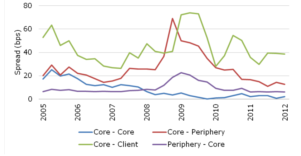
| Sample | Date | Bonds | affected | Time | |
|---|---|---|---|---|---|
| Phase 1 | July 1, 2002 | IG TRACE | eligible | bonds with issue size of | 75 |
| $1 billion | + | ||||
| Phase 2 | March 1, 2003 | All TRACE | eligible | bonds rated A- or higher | 75 |
| with $100+ | original | issue; 50 HY bonds | |||
| Phase 3A | October 1, 2004 | All bonds | BBB- or | higher | 30 |
| Phase 3B | February 7, 2005 | All bonds | BB+ or | lower | 30 |
5.7 Pre-trade transparency obligations for US corporate bonds
The conclusion from this analysis of detailed studies of the US corporate bond market is that that even without any regulatory requirement for pre-trade transparency, a degree of effective pre-trade transparency has been achieved through a combination of post-trade transparency (via the regulatory obligation for post-trade dissemination of transactions), and through competitive entry by new electronic platforms adapted to the natural fragmentation of the corporate bond market.[75] While the market remains dominated by broker-dealers and large buy-side intermediaries, the introduction of periodic batch auctions appears to have provided a degree of pre-trade transparency for some categories of bonds and at least for those issues have helped to reduce trading costs for large buy-side firms.
Still, in the US there are concerns that the structural transformation of the corporate bond market (and to an even greater degree the extremely fragmented US municipal bond market) has gone far enough and questions whether the benefits of lower trading costs for institutional investors are being passed on to small savers and primary issuers. These have been voiced by officials at the SEC (Securities Exchange Commission).
In particular, Commissioner Mary Jo White has pointed out that there is no equivalent for fixed income markets of the Regulation NMS (National Market System) which has been so influential in shaping the technological development of equity markets (see, SEC (2014)). While transactions prices for corporate bonds are transmitted fairly quickly to large institutional investors for most bonds pre-trade price information is limited to only some bonds and only on some venues. This is certainly not being disseminated widely. She argues that technology in fixed income markets has evolved too slowly and is largely limited to shedding light on inventory holding among the participating institutions. This has served to reinforce the position of the traditional players who have dominated the OTC market. She has argued for the introduction of some form of pre-trade transparency obligation.
Despite having a vocal advocate of stimulating greater pre-trade transparency, it is notable that in the US there has not been progress in finding a form for a regulation that would convincingly achieve that end and would not be susceptible to creating unintended consequences such as killing off the willingness of participants to hold and quote firm prices for issues that are naturally susceptible to adverse selection (i.e., older, smaller issues and HY issues). Also given the large numbers of securities involved, one can question whether complete pre-trade disclosure is of much practical use to retail or very small institutional investors who would be naturally ill-equipped to process the resulting large amounts of information. A more effective solution for retail investors may be to provide greater transparency of costs by paid by bond funds including ETFs.[76]
5.8 Transparency in the European corporate bond market
We have reviewed in some detail the experience of the US corporate bond market because the introduction of TRACE in 2002 was a major change that greatly increased the degree of post-trade transparency and because, thanks to TRACE, there has been a rich source of information that has given us insights into the effects of post-trade transparency, the nature of the dealer trading network in the market and the consequences of entry of new trading venues. We now turn the European corporate bond market and compare and contrast its experience with that of the US.
It is useful to recall some of the findings in the study by Biais et al. (2006) which was devoted to the issue of transparency in European corporate bonds. They emphasised the important differences between European corporate bond markets and other securities markets. The market is naturally fragmented with a very large number of issues which differ in a variety of dimensions. It is dominated by institutional investors who often engage in buy and hold strategies which naturally limit secondary market activity. Retail trading is relatively unimportant. Dealers are important in providing liquidity. The dominant market form is bilateral OTC trading among broker/dealers and between broker/dealers and institutional investors. At the time of their writing, platforms were minor providers of liquidity. In their view this market structure as a natural response to the inherent fragmentation of the corporate bond market.
Despite the fragmentation of European corporate bond markets they found that the market functions surprisingly well. They found evidence of active competition in the Euro denominated bond market, with spreads and other indicators of market liquidity that compare favourably with estimates for US markets made by other researchers. This was perhaps a surprising finding given that they also found that the European corporate bond market in 2006 was neither pre-trade nor post-trade transparent while in the US the market had been post-trade transparent since 2002. They found that sterling issues were less liquid than Euro issues and they attributed this to a lower level of competition among dealers in the sterling segment.
In their interviews with both buy-side and sell-side practitioners, they found little support for a regulatory initiative to force the development of new platforms or to impose an order-driven market structure. They were sceptical about the usefulness of regulatory imposition of pre-trade transparency. Indeed, they argued that it was hard to imagine that pre-trade transparency would work with a bilateral negotiation market structure. Instead, they argued that both theory and empirical evidence suggests that competition drives liquidity. The best way to promote liquidity would be to promote European market integration.
Regarding post-trade transparency, they argued that the evidence is ambiguous. Theory shows that more post-trade transparency with a given number of dealers would reduce spreads, but it would reduce profitability of dealing. If dealers withdraw from the market because of lower profitability, then this will widen spreads. So it is a matter of elasticity of supply. In their interviews, they found that buy-side practitioners either favoured post-trade transparency or were neutral. Sell side practitioners opposed it, arguing that it would discourage dealer’s liquidity provision especially for smaller issues.
On balance the authors recommended no pre-trade transparency obligation, but some additional post-trade transparency obligation but introduced cautiously using delays and no trade size transparency beyond a maximum reporting trade size.
While MiFID which came into effect in 2007 did introduce a pre-trade and post-trade transparency obligation for equity markets, it did not do so for bonds or for other nonequity instruments. However, it did introduce a reporting obligation for bond trades involving certain participants on European corporate bond markets. As a result, EUbased legal entities need to report transactions in European corporate bonds to the competent supervisory authorities.
Typically, the competent authority for a given corporate bond is determined by the legal location of the issuer of the bond. So for example, trades in corporate bonds issued by UK based companies need to be reported to the UK’s Financial Conduct Authority, trades in issues from French entities are reportable to France’s Autorité des Marchés Financiers, etc. As a practical matter, trades are reported by dealers to their home supervisor which in turn forwards the information regarding bonds for which they are not the competent authority to the appropriate supervisor via a central hub operated by ESMA.
However, it is important to note that these reports are destined only to the competent national supervisory authority and are accessible neither to other national regulators nor to regulatory bodies at the European level (e.g., ESMA). Furthermore, these data have not been available the public generally and thus have not be subjected to academic study as has been the case for TRACE data in the US.
While the transparency regime was not introduced for bonds with the introduction of MiFID, it does not mean that that the structure of the bond market has stood still in the last ten years. Indeed, as discussed in Section 4 of this report, there are forces that seem to be pushing toward changing the structure. Many market observers have argued that the market has been influenced by the global financial crisis and the regulatory response to it.
Also, very loose monetary conditions combined with the restrained bank lending have encouraged the growth of corporate bond issuance in Europe. Furthermore, from 2016 the ECB’s Corporate Sector Purchase Program (CSPP) has introduced a huge new player into the Euro denominated corporate bond market. (See Section 3 of this report). In addition to these factors, the developments of new trading platforms that are beginning to take hold in the US may be beginning to have a similar disruptive influence in European corporate bonds markets.
What is the evidence of a changing structure of the corporate bond market in Europe since the crisis? Unfortunately, the fragmentary nature of the information available about the corporate bond market has given us only partial answers to this question. The best data are in the hands of the regulators, and, as we have already discussed these have not been integrated across the various regulatory jurisdictions. However, on a number of points there seems to be a degree of clarity.
First, there is clear evidence that the size of the European corporate bond market has grown significantly since the crisis and now stands at levels that are significantly greater than pre-crisis levels. For example, for the data from the French regulatory authorities show that the French corporate bond markets nearly tripled in size between 2005 and 2015.
At the same time, there is evidence that European dealers have been reducing their inventories of corporate bond securities. For example, the FCA reports that in the UK inventories of dealers have declined from about £550 billion in 2009 to about £250 billion at the end of 2014. This strong decline of dealer inventories is similar to the findings for the United States as reported by the NY Federal Reserve (see Adrian et al.
(2015)). This official sector evidence gives support to the claims of sell-side practitioners that there has been a retreat from traditional principal-based market making at least for some categories of corporate bonds (see, ICMA (2016)).
In the face of strong demand for liquidity services driven by increases in issuance and declining supply of liquidity provision from principal-based OTC market making, it is natural to ask whether forms of liquidity provision have come through entry of new trading platforms and the involvement of institutional investors who have adapted their trading strategies to sometimes enter as providers of liquidity.
It is possible that changes to market microstructure of corporate bond market may have altered the information that various parties hold. We have discussed the development of electronic trading in Europe in Section 4 of this report. We found that the European corporate bond market appears to be evolving to incorporate elements of electronic trading. For now, this has been reflected mainly in the increased use of RFQ platforms to implement dealer to client trades. This protocol can help reduce trading costs by emulating the competitive environment of a sealed-bid batch auction.
But, there needs to be sufficient potential trading interest for this to work well. Until now the pace of change has been evolutionary rather than revolutionary. Potentially, recent efforts to mine information for pre-trade market discovery can change, however, this by overcoming the information disadvantage of major buy-side investors that would lessen the costs for them to begin to play as liquidity- makers as well as liquidity-takers.
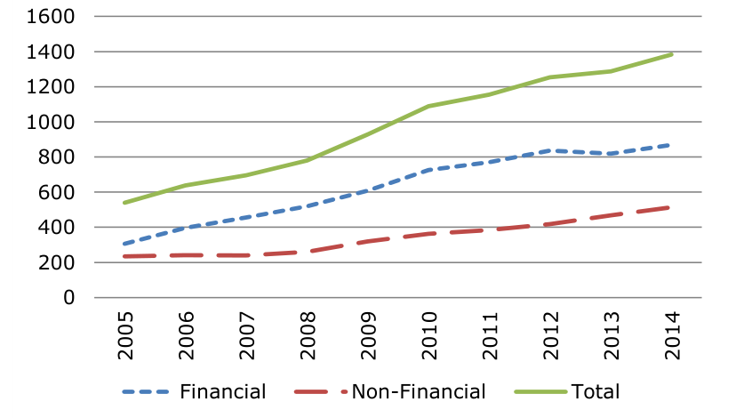
Note: The sources are AMF and authors’ calculations.
5.9 Implications of MiFID 2 and MIFIR implementation
This picture is set to undergo a major change through the implementation of MiFID 2 and the associated regulations contained in MIFIR. MiFID 2 was approved by the European Parliament and the Council in 2014. It is intended to extend to cash bonds and other non-equity instruments a pre-trade and post-trade transparency regime analogous to that which MiFID brought to European equities trading in 2007. The current time-table envisages that MiFID 2 will be transposed into national laws by July 3, 2017 and will become effective in January 2018.77
Part of the difficulty in settling the details of the new regulations reflects the very significant differences between the equity markets and the traditional market structures of cash bonds and other non-equity instruments. Many practitioners, on both buy- and sell-sides of the market, have argued that it would be very difficult impose the full transparency regime to the wide range of instruments and trading conditions that are found in the cash bond market, especially corporate bonds. As a result the proposed regulation standards allow for differences in the way the regime will work for instruments that are deemed “liquid” and those that are categorized as “illiquid”.
The post-trade transparency requirement is implemented through an obligation to publish information on completed transactions within agreed delay period. The MiFID legislation calls for publication as close to real-time as possible and in any case within 15 minutes following the trade for liquid instruments. This deferral limit would apply from the time the regulations enter into force in 2018 and are to be reduced in stages. Trades in illiquid instruments are to be exempted from this short delay standard but nevertheless will need published by 19:00 local time in the second trading day following the transaction (i.e., a 19:00 T+2 standard).
The general principle of the pre-trade transparency requirement for non-equity instruments is set out in Article 8 of MiFIR which requires trading venues to “(…) make public current bid and offer prices and the depth of trading interests at those prices which are advertised through their systems.” The requirement also applies to “actionable indications of interest”.
Under ESMA’s technical standards, pre-trade transparency may be waived for bonds that are classified as illiquid for the purposes pre-trade transparency or for offers to trade that are larger than an instrument-specific threshold.
Thus, for quote-based trading systems, firm quotes to buy or sell liquid issues in amounts below the size thresholds, the venue will be required to make publicly available information about the price, direction and quantity.
In the case of MTFs operating periodic batch auctions, it is expected that offers become actionable only at the end of the period during which responses to RTFs may be made. Thus, the pre-trade transparency obligation will kick in only from that point. Once a transaction is completed, the unexecuted firm quotes are no longer actionable and therefore will not be subject to disclosure in the pre-trade disclosure rule. (TBC)
This poses the thorny problem of how to classify instruments as liquid and illiquid for the purposes of the post-trade and pre-trade requirements. ESMA considered two possible approaches to this problem. One would place instruments into various categories based on issue and issuer characteristics and classify all instruments in each category either as liquid or illiquid. The alternative approach would be an instrument by instrument approach (IBIA) based on market observations.
The basic criteria for deciding whether a bond is effectively liquid in its trading experience are (a) average daily turnover of at least €100,000, (b) average number of daily transactions must equal or exceed a minimum initially set at 15 but scheduled to decline in stages to 10, 7 and ultimately 2, and (c) minimum number of days when the bond trades should be at least 80% of the trading days (European Commission (2016b), p.13).
In the end, ESMA has settled on the IBIA standard to be applied through an annual classification based on the preceding year’s trading experience.78 ESMA examined what these standards would imply for a historical dataset obtained from national regulators and found that more than 95% of European corporate bonds would be classified as “illiquid”.
The use of a one-year look-back for the purposes of classification then poses the issue of how a newly issued bond is classified for the first 12 months of its trading life. It is our understanding that this issue has not yet been totally decided. However, the ICMA (July 2016) study based on practitioner interviews states that the wide-spread expectation among practitioners is that all or almost all corporate bonds will be classified as illiquid.
Based on this summary of current plans for MiFID 2 implementation, we anticipate that initially the major effect the new pre-trade transparency regime will be felt by a relatively small number of comparatively liquid corporate bonds. For these bonds, we expect that liquidity as measured by frequency of trades may drop off as trading gravitates towards forms of negotiation that mitigate problems of information leakage. If subsequently the criterion for a liquid market is phased in as planned, these same pressures could be felt by a significant number of bonds. Ultimately, this could be a major driver of change in the microstructure of the European corporate bond market.
During the initial phase most bonds will be considered illiquid, and for these bonds the main effect of the new reporting regime will be felt through the post-trade publication obligation. This is on the assumption that details of price and quantity of individual transactions will be disseminated widely enough to be usable by all institutional participants in the market within about 48 to 72 hours of a transaction taking place.
This will give rather coarse information with a significant delay, but it will still be a significant increase in the degree of post-trade transparency to the market when compared to the situation that has prevailed in the European corporate bond market up until now. It will enable institutional investors and their data providers to better identify bonds that are more likely to be in the hands of broker/dealers and other active market participants who may be receptive to a request for quotes. And it will give an important point of reference that will serve to anchor the price discovery process for the market as a whole. This potentially can stimulate greater use of batch auction trading mechanisms and therefore indirectly induce a greater degree of pretrade transparency as well.
Depending upon the number of bonds that emerge in steady-state as liquid bonds subjected to strict pre-trade transparency, this may potentially increase pre-trade transparency for illiquid bonds through an indirect channel. Specifically, it may encourage the growth of benchmark referencing. This would encourage trading illiquid bonds on a yield relative to benchmark basis as is more widely practiced in US markets. This would imply a major evolution in European trading culture. So we consider this a possible future consequence of the new transparency regime but not necessarily very likely to occur. However, if the recent growth in primary issuance of
European corporate bonds proves to be a secular trend rather than a cyclical phenomenon, such a change in trading culture could well take hold.
6. Who holds European corporate bonds?
Summary of findings:
1. Systematic data collection on holdings of EU corporate bonds began only in
2014. We combine an analysis of this data with information of other data sources which provide evidence on long term trends.
2. The corporate bond market in Europe is supported by long-term institutional investors which seek future cash flows with predictable timing that can match the timing of these institutions’ liabilities. These investors are made up principally of insurance companies and banks. While pension funds are important in some member countries, for the EU as a whole, they account for a relatively small amount of holdings of corporate debt.
3. Over time, the composition of holdings has been shaped by two distinct trends. One is the growth of private collective savings vehicles in Europe. The second is the increase in globalised capital flows which means that a larger fraction of European corporate issues are in held by non-EU investors including foreign insurance and pension funds, sovereign wealth funds, and off-shore hedge funds and other alternative investment vehicles.
4. Both of these trends could eventually introduce a form of active portfolio management which may become a source of liquidity provision in the secondary market. This is because large fund managers, including those that are internationally active, operate at a scale that could justify investment in a larger, more sophisticated trading team. However, for now it is hard to see evidence of this happening. This may be because the trading style of these investors will change only gradually. Or possibly these forces for change have been obscured by the introduction of the ECB’s corporate bond purchase programme in 2016.
5. In an annex to the chapter, we provide a brief discussion of long-term trends in the US corporate bond market. Better data availability in the US facilitates the detection of some important trends in the composition of holdings of corporate debt.
6.1 Introduction
The market for corporate bonds serves to channel funds from savers to enterprises which use the funds to support on-going operations and for capital investments. In previous sections, we have looked in some detail at the functioning of the secondary market for corporate bonds which facilitates the passage of corporate debt issues into the hands of the ultimate providers of funds. In this section, we examine holders of corporate bonds, which may be household savers or, more likely, institutional longterm investors which invest funds on behalf of households. In particular, we are interested in identifying trends or patterns in the composition of these holders which could affect the nature of the secondary market.
6.2 Trends in European institutional fund management
To understand the evolution of European corporate bond holdings, it is important to grasp the fact that national capital markets have developed in very different ways across Europe. In some cases, institutional investing has been highly developed for some time while, in others, it has been rudimentary.
To illustrate, Davis (2008) reports the percentages of GDP represented in different European countries by pension funds, investment funds and insurers in 2000. The respective percentages were 81%, 27% and 52% for the UK and 111%, 25% and 65% for the Netherlands, showing the importance of pensions saving in these countries. For France and Germany on the other hand, the percentages were 7%, 55% and 61% and 16%, 12% and 43%. For southern European countries such as Italy, Spain, Portugal and Greece, the percentages of GDP represented by pensions were 3%, 7%, 12% and 4%. Investment funds were 39%, 30%, 16% and 25%, while insurers were 21%, 13%, 20%, and 1%, showing the poor state of development of insurance markets in these countries.
In two European countries, Ireland and Luxembourg, the investment fund management industry has been highly concentrated, reflecting accommodative taxation and relatively relaxed regulation. The assets of pension funds and insurers in these two countries were estimated to be 51%, 144% and 45% in the case of Ireland by David (2008) and 1%, 3,867% and 117% in the case of Luxembourg.
Recent developments have not altered the major differences across countries. Towers Watson (2016) compares the percentage of pension assets to GDP in different countries in 2005 and 2015. In the UK and Netherlands, the percentages rose from 79% to 112% (in the UK) and from 109% to 184% (in the Netherlands). On the other hand, in France and Spain the percentage remained flat at 6% and 3% respectively, while in Germany it rose from 10% to 13%. Noticeable in countries with strong defined benefit pensions industries was an increase in portfolio shares of bonds. In the Netherlands, the portfolio share of bonds went from 47% to 52% while in the UK, the rise was from 25% to 37% between 2005 and 2015 according to Towers Watson (2016).
Trends in European investment funds are hard to track but recent estimates by an ESRB study (Grillet-Aubert et al. (2016)) show that bond funds have been consistently the largest category of funds since 2009. Their estimates, which omit some EU countries (most notably the UK), show the total size of bond funds rising from €1.5 trillion in 2009 to about €2.8 trillion in 2015. Equity and mixed funds grew by similar percentages while, in contrast, money market funds slightly declined.
The strong trend of growth of assets under management in recent years is partially explained by the decline of interest rates as the ECB and other monetary authorities pursued expansionary monetary policies. The inflows of new money into bond funds is also documented by Grillet-Aubert et al. (2016) who show substantial net issuance of shares in various categories of funds since 2010, notably in bond funds in the period 2012-14 (coinciding with strong growth of the primary market issuance).
Data from EFAMA (see EFAMA Quarterly Statistical Release (2016) Q2) also show a substantial rise in the net assets of Undertakings for Collective Investments as Transferable Securities (UCITS) over the period 2010 to 2015. In this category of funds, assets under management rose from Euro 1.4 trillion to Euro 2.1 trillion over the period. Again, money market funds declined somewhat while equity funds rose from Euro 2.1 trillion to Euro 3 trillion over the period.[79]
The figures reported by EFAMA on bond holdings do not distinguish between sovereign, corporate, and other types of bonds. The ESRB study by Grillet-Aubert et al. (2016) provides estimates of non-financial corporate bonds in the EU held by investment funds (including money market funds), monetary financial institutions (including banks and central banks but excluding money market funds), and insurance companies and pension funds. The results, reported in Figure 6.1, show a strong increase in holdings by investment funds from €150 billion in 2008 to nearly €350 billion in 2015. This more than compensates for the decline in banks’ holdings which amounted to about €100 billion over the same period.
The data sources summarised above suggest that strong trend growth in European institutional investments has provided a strong natural source of demand for the corporate bond market in Europe. In contrast to the US (see the annex to this chapter), pension funds have been a relatively less important market for corporate bonds.
There has been a strong long run growth in collective investment funds, in particular UCITS, aimed at the retail market in Europe, and much of this market has been concentrated in bond funds. While data are incomplete, there are indications that this has been a strong source of demand for European corporate bonds since the crisis and, especially, between 2012 and 2015.
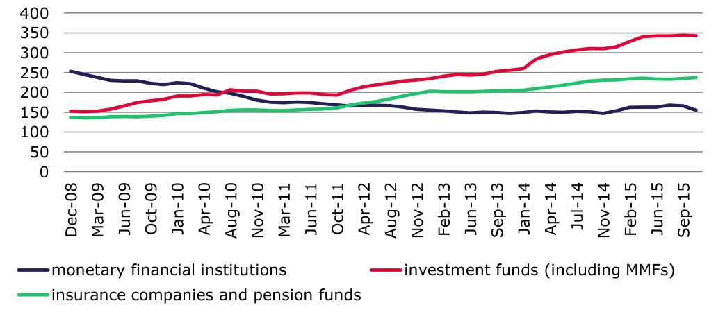
Note: The source is ECB. Data is in Euro billions.
6.3 Corporate bond holdings in the Euro zone
The difficulty of obtaining a comprehensive picture of the European corporate bond market (as well as other aspects of the non-bank financing in Europe) has been the lack of flow of fund statistics providing sources and uses of funds on a standardised basis throughout Europe. This situation is changing as the ECB has started to publish statistics on holdings in 2014.80The ECB’s Securities Holding Statistics (SHS) data have been collected quarterly since the fourth quarter of 2013 and cover the two main types of securities: debt securities and equity securities (including investment fund shares).
Aubert et al. (2016). The discrepancy may in part reflect the fact that the latter study included bond funds managed as alternative investment vehicles. 80 For a description see ECB (2015).
An important feature of this dataset is that holding information is collected at the level of each individual security, i.e. security by security. From this it is possible to report the holdings information at different levels of aggregation depending upon the application. For example, this can be used to construct flow of funds tables at the national level, such as in reporting holdings of debt and equity instruments issued by various categories of French domiciled entities that are held by other French domiciled entities and “the rest of the world” which in this context would include non-French entities in the EU. Alternatively, it can be aggregated to cover the euro zone (EU-19) countries which report financial claims issued by entities in the euro zone held by categories of entities in the euro zone and “the rest of the world”, which in this context would include non-euro zone countries in the EU.
The SHS (Securities Holding Statistics) Sector module encompasses two main distinct sets of data: (i) holdings of securities by investors resident in the euro area, such as households in Germany or monetary financial institutions (MFIs) in France, and (ii) non-resident investors’ holdings of euro area securities that are deposited with a euro area custodian, such as US investors’ holdings of German securities deposited in Luxembourg. In addition, most non-euro area EU countries (namely Bulgaria, the Czech Republic, Denmark, Hungary, Poland and Romania) also collect SHS Sector data. The fact that the fund management industry is highly concentrated in Luxembourg and Ireland means that the omission of the UK from the SHS is not as serious as it might be otherwise. This is because a large fraction of holdings by funds would be reported through entities in those two countries and thereby included in the SHS.
6.4 ECB data in multiple forms
The ECB provides rich but partial information for holders of debt issued by sectors in different countries. The data departs from FISMA’s preferred data breakdown in that it does not cover all 28 EU countries and because the sectoral breakdown fails to distinguish some categories. In this section, we set out adjustments that permit one to deduce breakdowns in holdings over time for all 28 EU countries. In future work, we shall focus on making the sectoral breakdown closer to that desired by FISMA.
European Central Bank Securities Holdings Statistics (SHS) have been collected by ECB on debt securities, equity securities and investment fund shares. The data is collected on a security-by-security basis. Reporting agents report a few essential items, such as the International Securities Identification Number (ISIN) and monetary amounts (positions and/or transactions) to the statistical authority. SHS data has two sub modules: SHS-Sector data and SHS-Group data. We are mainly interested in the Sector data.
The SHS data is published by the ECB in three aggregated versions:
• The first of these is also called ‘SHS’. In this aggregated ‘SHS’ form, the data consists of ‘total economy’ holdings with no sector breakdowns either for issuers or holders.
• The second aggregate form consists of Euro area financial and non-financial accounts (EAA) ‘who-to-whom’ data. These ‘who-to-whom’ data identify both the creditor and debtor for a financial transaction or position. From ECB (2015), we learn that ‘An extension of the who-to-whom coverage to all marketable instruments, namely debt securities, quoted shares and investment fund share, will now be possible thanks to the detailed information contained in the SHS’. This indicates this ‘who-to-whom’ data is derived from the SHS data.
• A third aggregate form of the SHS data consists of the ECB’s ‘aggregated balance sheet data’. This account data is what we primarily employ. It has the drawback that some of the sector classifications differ from what FISMA would prefer. Table 6.1 shows the financial sectoral breakdowns available in the ECB sectoral balance sheet data and what FISMA would prefer to see. Note that FISMA wishes to see holdings by Undertakings for Collective Investment in Transferrable Securities (UCITs) funds and alternative investment funds.
The availability of the data lying behind the aggregate balance sheet data is summarised in Table 6.2. Better data are available for the Euro area than for other countries. Debt issued by Euro area entities is covered so long as their holders are in one of the 19 Euro area countries or in one of an additional group of six countries. If their holders are from Slovenia or the UK, Euro area issues are only included if they are reported by Euro area custodians.
Holdings of non-Euro area bonds are only included if they are held by Euro area countries or countries in the additional group of six. Otherwise, they are not reported. Figures on holdings by the rest of the world may be inferred as residuals but, as such, as combined with other excluded categories, such as UK holdings of Euro area debt not held through Euro area custodians.
There remain problems with regard to the completeness of the data that are reported to the ECB, hence data gaps and inconsistencies are undoubtedly present. Data that the ECB identifies as missing include holdings of Euro area bonds by United Kingdom, Sweden, Croatia- investors that are not under Euro area custodians. ECB document states ‘SHS coverage of holdings by non-Euro area investors reported by Euro area custodians is also relatively high, around 81%’. On omitted reporting, ECB documents state that debt reporting covers 92% of the amount of outstanding of debt securities issued in the euro area.
| ECB classification | Preferred |
|---|---|
| Monetary financial institutions | Banks |
| Insurance corporations | Private |
| Pension funds | Insurance |
| Non MMF investment funds | Pension |
| Other financial institutions | Asset |
| Hedge funds |
| Table 6.2: Reporting scope | by geographical area | |
|---|---|---|
| Issuer domicile | ||
| Holder domicile | Euro area | Non-euro |
| Euro area (19 countries) | Reported | Reported |
| 6 non-Euro EU countries | Reported | Reported |
| Other countries | Reported by Euro area | Not reported |
| custodians only |
Note: 6 non-euro EU countries include Bulgaria, Czech Republic, Denmark, Hungary, Poland and Romania.
6.7 Corporate bond holdings in the EU
6.7.1 Euro 19 results
The analysis in the preceding subsection gives us an insight into who holds long-term debt issued by Euro zone entities. However, it does not tell us the composition of holdings of long-term debt issued by all entities based in the EU. In order to shed light on this issue, we have combined information contained in the flow of funds accounts for the Euro zone countries with information from sectoral financial balance sheets for the remaining nine EU members in order to estimate a flow of funds table for the EU as a whole.
The basic assumption that we make in doing this is that the pattern of holdings across EU19 holding categories that holds for EU19 issue categories can be extrapolated to EU28 issues for the same issue category. Under this assumption, we can use information from aggregate national balance sheets for the non-euro zone member states broken down by issuer category to arrive at an estimate of holdings for the EU as a whole.
Figure 6.2 shows holdings of bonds issued by Euro 19 countries for Q4 2013 and Q2
2016. Individual histograms present the holdings (broken down by sector of domestic holders and by rest of the world) of bonds issued by the different issuer sectors: nonfinancial corporations, insurers, MFIs, and other financial institutions. (Issues by pensions, households and investment firms are too small to be of interest.) The statistics shown in Figure 6.2 are taken directly from ECB data and do not require manipulation or calculation. Table 6.3 shows figures for holdings for Q2 2016.
The Figure 6.2 results show that for non-financial corporation issuers, the key investors are Euro 19 non-MMF investment funds, insurers and MFIs, i.e., the banking sector. The rest of the world (which here, of course includes EU investors outside the Eurozone as well as non-EU investors) are also very important.[81] It is noticeable that non-MMF investment funds and insurers significantly increased their holdings between Q4 2013 and Q2 2016 (as did the rest of the world) whereas the holdings of Euro 19 MMFs were flat. The holdings of other sectors were both minor and relatively flat although the small fraction held by other financial institutions did grow considerably in proportional terms between the two dates.
The insurer bond issues shown in Figure 6.2 are a small fraction of those issued by non-financial corporations. For reasons which would need to be explored further, the ECB statistics suggest that rest-of-the-world holdings of Euro 19 insurer bonds are negligibly small. Euro 19 insurer bond issues are held mainly by other Euro 19 insurers, MFIs and non-MMF investment firms. Again, MFI holdings have been flat while insurer and investment firm holdings have grown significantly in recent years.
Figure 6.2 shows that MFI bond issues comprise much of the largest category of Euro 19 bonds. For example, they are about three times greater than those issued by nonfinancial corporations. Monetary financial intermediaries (MFIs) here include money market funds but principal liabilities of the MMFs take the form of shares rather than bonds and are, therefore, not included in the statistics displayed here.
Euro 19 MFI bond issues are mainly held by other euro 19 MFIs (of the €3.9 trillion outstanding bonds issued by MFIs, about €1.5 trillion are held by other MFIs) and by the rest of the world.[82] Total MFI bond issues have actually fallen between Q4 2013 and Q2 2016. Euro 19 MFI bonds are the only category (among the four categories that we examine) for which the household and non-profit holdings are significant. These have fallen noticeably in the period covered by the histogram. It is likely that the structure of MFI bond ownership in part reflects the structure of a number of major banking groups which in part have emerged as groups of banking cooperatives in the past.
Other financial institution Euro 19 bond issues are also very large (compared with nonfinancial corporate and insurer issues, for example) and show similar patterns of ownership as euro 19 MFI issues. (Note that the large amounts of issues outstanding of “other financial institutions” include largely securitization.) One difference with Euro 19 MFI bond issues is that rest of the world holdings of euro 19 other financial institution bonds rose significantly between Q4 2013 and Q2 2016.
Table 6.4 provides another view of trends in Euro 19 country bond holdings over time, showing holdings of bank and non-financial corporation bonds between 2013 and Q2
2016. Over this period we see that investment funds and insurance and pensions funds have been increasing their holdings of non-financial corporate bonds while banks have been just maintaining or slightly reducing their holdings.
The evolution of holdings of bonds issued by euro zone banks has been rather different. An interesting and surprising finding from this table is that households which held nearly €700 billion of Euro zone bank debt in 2013 have reduced their holdings by about €300 billion since then. Insurance companies and pensions funds and banks have also reduced their holdings of euro zone bank bonds but at a more moderate rate.
Finally, Figure 6.3 shows the breakdown of Euro 19 country sector holdings broken down by issuer in Q2 2016. MFIs hold the most, followed closely by the rest of the world and then by insurers and non-MMF investment funds. In all these cases, the largest issuer contribution to holdings is by MFIs. But insurers and non MMF investment funds have relatively large holdings of non-financial issuer bonds. In fact, MFI holdings of non-financial bonds are the fourth largest. Households appear surprisingly large holders and mostly own MFI bonds.
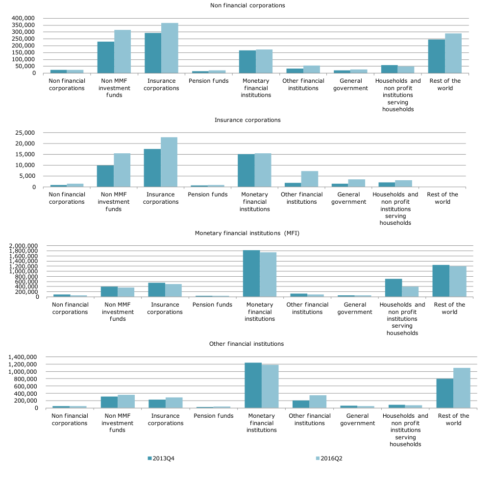
Note: This figure presents Eurozone holdings of debt securities issued by Eurozone entities. Each sub-chart represents one particular issuer sector and all its holding sectors. ‘Rest of the world’ represents non-euro countries’ holdings of debt securities issued by the 19 euro countries’. Holdings are in millions EUR. ‘Rest of the world’ holding is from ECB ‘who-to-whom’ data.
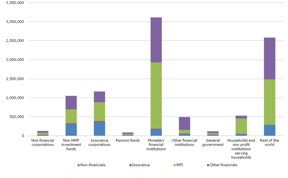
Note: This figure presents euro zone’s holdings of debt securities issued by euro zone entities. Each stacked bar represent one particular sector’s holding broken down by issuer sectors. ‘Rest of the world’ represents non-euro countries’ holdings of debt securities issued by the 19 euro countries’. Holdings are in millions EUR. ‘Rest of the world’ holding is from ECB ‘who-to-whom’ data.
| 2016 Q2 | Liabilities | ||||||||||
|---|---|---|---|---|---|---|---|---|---|---|---|
| Total | Non- | MFIs | Non-MMF | Other | Insurance | General Households | Rest of | ||||
| financial | investment | financial | corporations | government | the | world | |||||
| corporations | funds | institutio | and | pension | |||||||
| ns | funds | ||||||||||
| Total | 21,142 | 1,258 | 3,913 | 7 | 3,317 | 68 | 8,604 | 0 | 3,976 | ||
| Non-financial corporations | 195 | 19 | 33 | 0 | 33 | 1 | 72 | 0 | 37 | ||
| MFIs | 6,679 | 134 | 1,488 | 0 | 1,134 | 15 | 2,960 | 0 | 948 | ||
| Non-MMF investment funds | 3,852 | 306 | 343 | 0 | 342 | 15 | 896 | 0 | 1,950 | ||
| Other financial institutions | 794 | 55 | 69 | 0 | 322 | 6 | 244 | 0 | 97 | ||
| Insurance corporations and pension funds | 3,830 | 381 | 501 | 0 | 304 | 24 | 1,883 | 0 | 737 | ||
| General government | 412 | 24 | 44 | 0 | 44 | 3 | 194 | 0 | 103 | ||
| Households | 801 | 50 | 394 | 0 | 73 | 3 | 178 | 0 | 105 | ||
| Rest of the world | 4,581 | 289 | 1,041 | 7 | 1,066 | 0 | 2,177 | 0 |
Note: The table illustrates the basic structure of the ECB “who to whom” data. It shows holdings of long-term debt securities issued by euro zone entities and held by euro zone entities and by the “rest of the world” (which here includes entities in non-euro zone member countries and by non-EU entities to the extent that their custodians are in the euro zone or otherwise participating in the SHS framework.) Source: ECB Statistical Data Warehouse, Who-to-Whom Detail http://sdw.ecb.europa.eu/reports.do?node=1000002345
| 2015 | 2015 | 2015 | 2016 | 2016 | |||||
|---|---|---|---|---|---|---|---|---|---|
| Total long-term debt | securities | 2013 | 2014 | Q2 | Q3 | Q4 | Q1 | Q2 | |
| Liabilities of | non-financial | corporations, assets of: | |||||||
| Non-financial corporations | 18 | 19 | 19 | 19 | 20 | 18 | 19 | ||
| Monetary financial | institutions | 147 | 134 | 129 | 130 | 131 | 127 | 134 | |
| Non-MMF investment | funds | 222 | 261 | 274 | 272 | 279 | 287 | 306 | |
| Other financial institutions | 30 | 55 | 54 | 57 | 54 | 56 | 55 | ||
| Insurance corporations | and | pension funds | 303 | 337 | 335 | 346 | 357 | 368 | 381 |
| General government | 19 | 23 | 23 | 23 | 24 | 24 | 24 | ||
| Households | 57 | 54 | 50 | 50 | 50 | 51 | 50 | ||
| Rest of the world | 221 | 274 | 279 | 272 | 282 | 279 | 289 | ||
| Liabilities of MFIs, | assets | of: | |||||||
| Non-financial corporations | 53 | 48 | 38 | 35 | 33 | 31 | 33 | ||
| Monetary financial | institutions | 1,598 | 1,515 | 1,497 | 1,492 | 1,467 | 1,483 | 1,488 | |
| Non-MMF investment | funds | 360 | 381 | 362 | 357 | 343 | 343 | 343 | |
| Other financial institutions | 72 | 84 | 87 | 85 | 80 | 87 | 69 | ||
| Insurance corporations | and | pension funds | 564 | 559 | 544 | 532 | 526 | 511 | 501 |
| General government | 51 | 50 | 49 | 50 | 44 | 45 | 44 | ||
| Households | 686 | 543 | 472 | 458 | 434 | 416 | 394 | ||
| Rest of the world | 1,109 | 1,110 | 1,130 | 1,085 | 1,074 | 1,041 | 1,041 |
Note: The source is ECB Statistical Data Warehouse, Who-to-Whom Detail. This is available at the address http://sdw.ecb.europa.eu/reports.do?node=1000002345
6.7.2 EU results
Figure 6.4 presents preliminary results of our analysis of EU bond holdings. The histograms follow the same format as in Figure 6.2 but are based on data calculated using the methodology explained in the last section. The data displayed comes from the Euro 19 countries, several minor countries and a single country with substantial financial markets, the UK.
As one might expect, the patterns of rest-of-the-world ownership are somewhat different when the UK and other non-euro 19 countries are included. A smaller fraction of bonds issued by EU non-financial corporates are held by rest of the world than is the case for Euro 19 countries. The surprising result that no Euro 19 insurer bonds are owned by the rest of the world is reversed when one considers the wider EU group of countries presumably because UK insurer bonds are held by non-EU countries. Larger fractions of EU MFI and other financial bonds are held by the rest of world than is true for Euro 19 MFI and other financial institutions. Many of the qualitative features of the Euro 19 country results remain valid with the EU countries. There are some differences, however. For example, the substantial proportional increases between Q4 2013 and Q2 2016 in investment firm and insurer holdings of non-financial corporate and insurer bonds evident for the Euro 19 countries are mitigated although smaller rises are still evident for bonds at the EU level.
The behaviour over time of the other financial institution holdings are also somewhat different when viewed at the EU rather than the Euro 19 country level. This is not surprising given the relative importance within Europe of the UK securitisation market.
Altogether, and despite the differences just highlighted, there is clearly much continuity between the results for EU countries and those for Euro 19 countries.
Figure 6.5 replicate the presentation of Figure 6.3 but for EU holdings in their entirety. Note that the scale of the plot is greater than Figure 6.3 in that the vertical axis extends to EUR 5 trillion rather than EUR 3.5 trillion. MFI holdings are EUR 5 trillion rather than EUR 3.1 trillion. The rest of the world is a smaller holder of bonds understandably as it no longer includes the UK. Again, insurer and non-MMF investment funds represent larger holders of non-financial bonds than do MFIs. Pension funds remain very small holders despite the inclusion of the UK with its large pension fund sector.
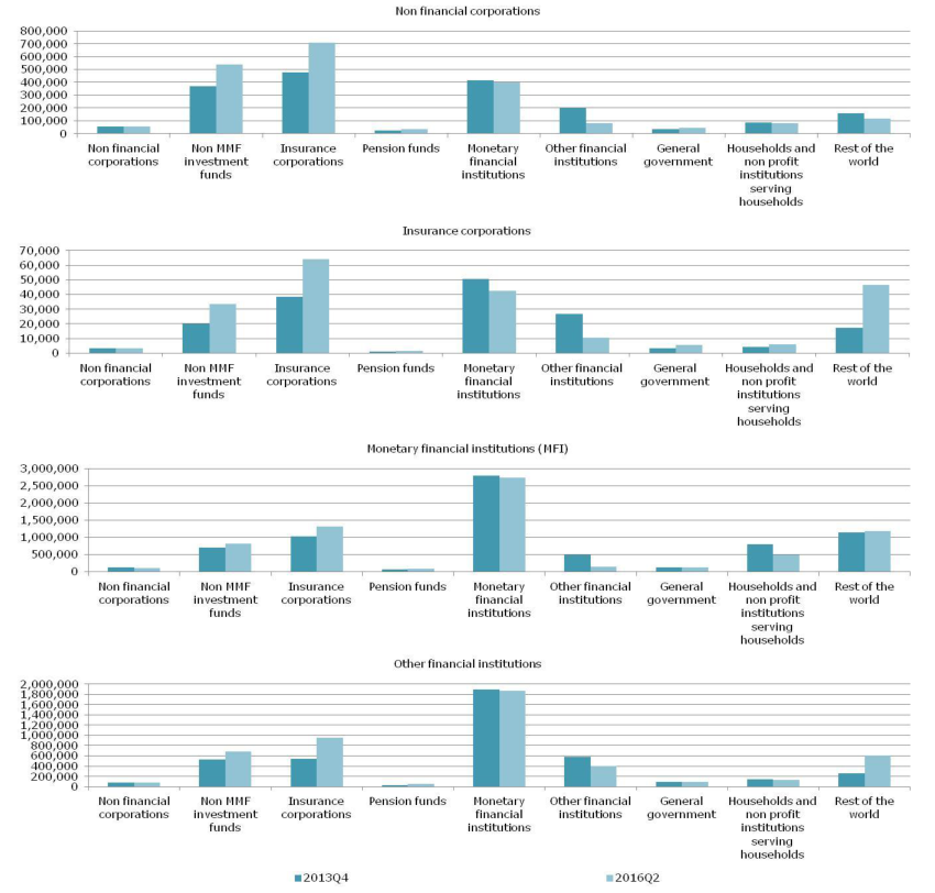
Note: This figure presents EU’s holdings of debt securities issued by EU entities. Each sub-chart presents the holdings of bonds issued by one particular sector. ‘Rest of the world’ represents non-EU countries’ holdings of debt securities issued by the 28 EU countries. Holdings are in millions EUR.
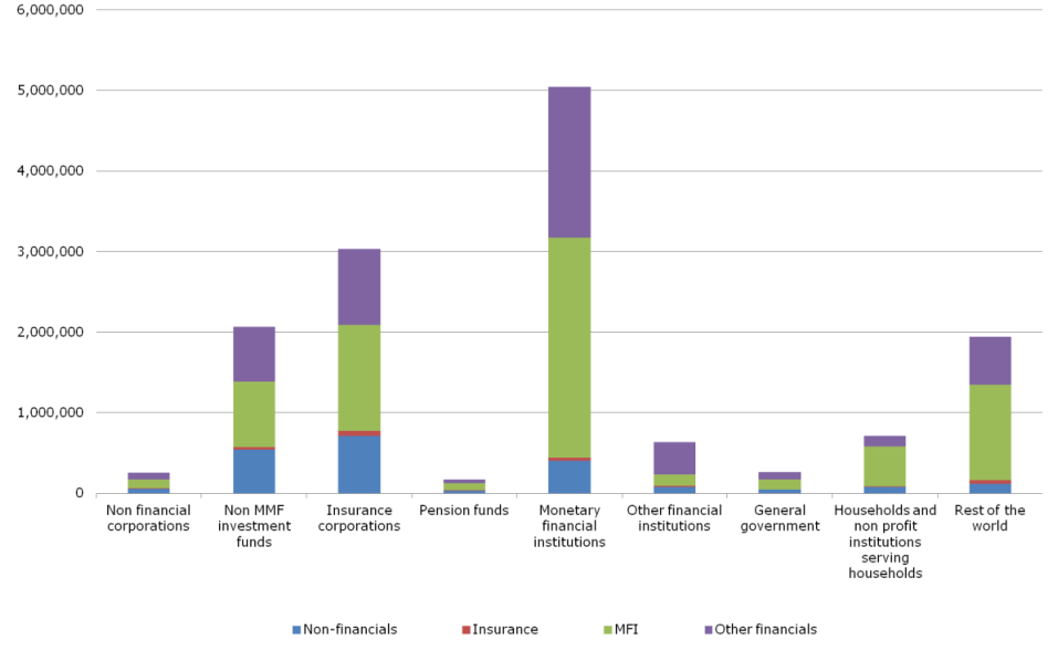
Note: This figure presents EU countries holdings of debt securities issued by EU entities. Each stacked bar represent one particular sector’s holding broken down by issuer sectors. ‘Rest of the world’ represents non-EU countries’ holdings of debt securities issued by EU countries’. Holdings are in millions EUR.
6.7.3 ISIN-level analysis of the SHS data
An important feature of the SHS data is that the basic data is reported for individual securities (ISIN’s) by entities with a reporting obligation. This means that potentially the determinants of demand for various categories of agents can be explored using multiple regression analysis and other powerful statistical techniques. To our knowledge, this feature was exploited for the first time by Boermans and Vereulen (2016), the authors of which are researchers at the Dutch central bank. Currently, access to security level holdings data is restricted to official sector analysts, but given the richness of the data, it is hoped that this data source can be made available to academic researchers and other analysts. Given that the data could be aggregated for different categories of holding entities, it is unlikely that this would be of limited use for proprietary trading or other commercial uses.
The focus of the Boermans and Vermeulen study is to identify the degree of home bias in investment preferences on various categories of investors. The approach they take is to estimate a form of multiple regression model, sometimes called a gravity model, which includes various measures of “distance” between the issuer and the investor. They implement this model for bonds and for equity holdings using five categories of investors: banks, pension funds, insurance companies, investment funds and households.
These regressions suggest that there are three factors which impact positively upon all categories of Euro zone investors’ appetites for a bond issue, namely size of issue, strength of the trading relation between the issuer’s domicile and the investor’s domicile and the fact that it is a Euro denominated issue (i.e., absence of currency risk for both the issuer and the holder). Insurance companies and pension funds give some evidence of having a pure home bias among bond issuers. Insurance companies and households have a preference for long-term issues. Banks and households have an appetite for floating rate issues, while insurance companies prefer fixed rate issues. All institutional investors seem to like covered bonds; while, households do not. Banks, insurance companies and investment funds have a liking for bonds that are eligible as collateral in ECB liquidity operations.
All in all, this is a most interesting paper. One hopes that the SHS data can be further explored provide insights on other factors which may aid our understanding of European bond market. In particular for our purposes it would be most interesting to see the results of similar regression applied to the European corporate bonds along with a break-down between issues of non-financial corporations and financial intermediaries.
For more detail on trends in the US corporate bond market, see Annex 3. For more information on the ESA’s classification of terms, see Annex 4.
7. What are the Drivers of Dealer Profitability?
Summary of findings:
1. This section examines proxies for dealer profitability and discusses possible determinants of their variation over time.
2. Using FCA data, we are able to construct measures of round-trip returns for individual banks and ISINs. We presents gross returns averaged across banks and bonds and then adjust for funding costs, and interest rate risk.
3. The resulting net adjusted returns are closely correlated with returns on a widely used European Investment Grade bond index. We regress on this return to proxy for the effects of book-level hedging and show that round trip returns have trended down over the sample period.
4. We present other proxy indicators of dealer profitability including dealer inventory levels and carry yields. We discuss the dynamics of these indicators in relation to changes in banking regulation that have occurred in recent years.
5. We conclude that the timing of regulatory changes does not obviously square with the dynamics of profitability indicators. Regulatory capital has been relatively constant throughout the period we study and hence is less likely to have been the source of changes. Liquidity regulations are a possible source of declines in dealer inventories but causal connections are hard to establish.
7.1 Introduction
Post crisis changes in banking regulation and the current low interest rate environment are thought by many market participants to have affected banks’ incentives to make markets in European corporate bonds. The exact scale and nature of dealers’ engagement in corporate bond dealing is hard to assess but evidence on dealer inventories suggests that banks have reduced the scale of their dealing activities.83
Directly observing dealer profitability in a particular market such as European corporate bonds is difficult. Even within a fixed income trading operation, a bank may not know the true P&L attributable to particular desks. Hedging is often done at the level of the book and, hence, the costs of hedging cannot easily be attributed to specific activities. Desk level earnings are estimated for the purpose of calculating bonuses on the basis of the so-called “sales credit” system. Under this system, contribution to profits is estimated by applying weights to turnover. The determination of weights is opaque. One senior banker with whom we talked compared the resulting estimates to air miles.
Leaving aside hedging costs, one may estimate the profitability of trades based on round-trip analysis. This is done intermittently by some banks but is not implemented on a systematic basis by any bank that we questioned. Round trip analysis allowing for hedging is more applicable in the case of high yield bonds for which hedging is commonly performed at a single name level. But, where hedging is performed using credit indices, round trip analysis only provides a limited idea of profitability.
As an alternative to holding positive inventory to satisfy client demand, a marketmaker may meet a client order by borrowing a bond or obtaining it via a reverse repo. In this case, the calculation of profitability is more complicated yet. A market-maker selling a bond in such circumstances may have a month to cover their position. The counter-party may call in the bond or refuse to roll the repo so the market-maker is in danger of being squeezed. If the position cannot be covered quickly, the market-maker is highly likely to make a loss on the trade.
While precise identification of profitability is difficult, costs and their drivers are also somewhat opaque. For individual market-making desks, the cost of funding provided by the bank’s Treasury is generally transparent (although the funding rates are frequently much higher than the bank’s market cost of raising funds) but the capital consumption of trading positions will only be observed at the level of senior management.
Here, we examine the issue of dealer profitability indirectly by studying proxy measures. The first such proxy is round trip returns on purchase of individual ISINs by dealer banks. We construct these using FCA data which shows what for each individual institution has bought and sold for each ISIN. We focus on the ten largest dealer banks (by numbers of transactions) and ISINs with at least 200 transactions in the whole period. We report monthly averages of round trip returns across banks and individual bonds.
The second proxy we examine is the behaviour of inventories. The evolution of inventories reflects how profitable it is for banks to commit capital to dealing operations. The data we employ is based on the survey based estimates already briefly discussed in Section 2 provided by Grillet-Aubert et al. (2016).
A third proxy is an estimate of the carry return of holding bonds net of financing costs. For a large set of bonds present in the FCA dataset, we calculate the yield spread and subtract financing costs. Our estimates of financing costs reflect the funding costs faced by the bank plus managerial adjustments that bank treasury operations use to drive the balance sheets of their institutions.
What are the potential pressures on dealer profitability that would affect marketmaking profitability? During the period we study, major changes occurred in the regulatory environment that European bond market-makers face. The changes include the introduction of Basel 3 measures for bank capital, leverage and liquidity rules, and alterations in securities markets regulations.
The period we examine also contains the aftermath of one crisis (the 2007-8 subprime collapse culminating in the failure of Lehman Brothers) and the occurrence of a second major crisis: the 2011-12 European sovereign debt crisis which brought with it concerns about the durability of the Eurozone itself. These shocks to the market environment clearly affected dealer profitability considerably.
Other potential pressures on dealer profitability include the low interest rate environment that has prevailed in Europe since 2012 and, possibly, changes in the competitive environment.
7.2 Indicators of profitability
In this section, we display the indicators or proxies for market-making profitability that we will study. The first consists of round trip returns.
These returns are calculated using data for purchase and sales of individual ISINs by single dealer banks. Following each individual bond purchase by a bank, we track the subsequent sales and calculate what return was made. If the bank makes a second purchase before the first block is completely sold, we assume the second block remains in the bank’s portfolio until all of the first block is disposed of. This approach yields rigorous measures of round trip returns. The only failing of our approach is that it ignores the fact that the bank may have an inventory of the bond in question before the first purchase that appears in our dataset.
The above described round trip return is expressed as a percentage of the initial purchase price. We subtract from this “gross” round trip return the funding cost to obtain a net round trip return.
The funding cost is calculated by assuming that the bank pays for each of the subblocks that it sells the amount of the sale times the funding rate times the period of time between the purchase and the sale in question. The funding rate is assumed to equal a Euribor or Libor 1-year rate. If this falls below zero, we floor the rate at this level.
We track the round trip chains for three months, ignoring chains that remain unclosed in the sense that sales exhaust the purchase after that period. We experimented with calculations in which we tracked chains for up to six months. The time pattern of the average round trip returns was very similar in this case to those obtained assuming a three month cut off. There was slightly more scope for large losses when chains lasting up to six months were considered in that the time series plot showed returns from -4 to +3 percent instead of the range of returns from -3 to +3 percent that was obtained using a three month cut off assumption.
We also adjust for interest rate risk by calculating the return on a notional default free bond having the same contractual cash flows as the defaultable corporate bond in question. We price this default free bond using Euro or sterling denominated Treasury rates. We calculate these returns for each of the sub-blocks involved in a particular sale and work out and subtract from the purchase to sale return the equivalent return on the notional default free bond.
Figure 7.1 shows the gross return and the gross adjusted return for all bonds and the same quantities by age of bond. One may observe that the adjustments for funding cost and interest rate risk have some effect on the time path of average returns but not a substantial impact.
The plot suggests that returns both gross and net adjusted trend down apart form a spike at the end. Upon inspection the sharp negative returns close to the end of the sample period are associated with the default of some Portuguese bonds whereas the very marked positive spike occurs when the ECB announces its corporate bond purchasee program.
We calculated the gross and net returns broken down by sector (financial vs nonfinancial), rating, currency, country, IG vs HY and issue size. None of the categorisations led to very substantially different returns. As one may observe from the plots in 7.1.3 and 7.1.4, age has some effect especially when the volatility of return is great.
Figure 7.2 shows a similar breakdown of plots as in 7.1 but this time for the ”holding periods”, i.e., the average length of time between purchase and final sale (i.e., the completion of the round trip chain). Figure 7.2.1 shows that the average time period rise from about 25 to about 35 days over the sample period. (When we calculate chains allowing for completions of the chain over periods of up to six months, the time profile of the holding periods shows a similar shape but achieves highs of up to 65 days.)
The upward trend is also apparent in Figure 7.2.2 which breaks down the averages by age of bond. The rises are most obvious for older bonds which, in any case, exhibit higher levels than the young bonds. Again, the plots by HY vs IG and by currency show similar time profiles.
Finally, Figure 7.3 shows the behaviour over time of the average numbers of sales involved in chains. The number of sales for all bonds (in 7.3.1) falls sharply between 2011 and 2013 and is then fairly flat. Broken down by age, the declines appear more progressive and smooth over time despite some fluctuations. High Yield bonds show higher numbers of sales than Investment Grade (see 7.3.3) while currency and other break downs (not shown) appear to make little difference.
To investigate further the effects of adjusting the gross round trip returns first for funding costs and then for interest rate risk, in 7.4 we plot the three series for “all bonds” on the same graph. It is apparent how little difference the funding adjustment makes while the interest rate adjustment only affects the net returns to an appreciable degree for brief periods in mid 2013 and mid 2015.
Having adjusted for interest rate risk, the remaining adjustment one might make is for hedging. Corporate bond dealing books are commonly hedged at the bond level. (Some High Yield positions may be hedged at the security level.) To reflect hedging, we regress the total return series on the returns on a Bloomberg European Investment Grade bond index. Figure 7.5 shows the time paths of the index return and the net adjusted return on the same graph. It is apparent that many of the turning points coincide.
Table 7.1 shows the results of the regressions on the index return and time. We include two sample periods to allow for the fact that the ECB’s corporate bond purchase program represents a substantial potential regime shift. In both cases, the coefficient on the index return is close to unity and highly significant staistically. With the longer sample period, the coefficient is 0.99.
The coefficient on time in the aggregate regressions shown in Table 7.1 are negative, sizeable and highly statistically significant. The left hand side variable is in percent and the time variable is scaled so that five years equals one period. Hence, over the sample period, the return trends down substantially. Figure 7.6 shows a time plot of the residuals of a regression of the net adjusted return on the index return alone, showing the effects of the negative time trend.
The final exercise we perform with the round trip data is to run panel regressions of the individual round trip returns on index returns, time and bond characteristics. The results for net return and net adjusted return regressions are shown in panels a) and
b) of Table 7.2.
The first regression is just on the index return and time. As in the aggregate regression, the time trend is large in absolute value, negative in sign and statistically significant. The coefficient on the index return is again very close to unity in the simple regression for the net return. When more variables are added, again the time trend is negative and strongly significant.
The second proxy for dealer profitability that we consider is dealer inventories. Figure 7.7 shows European market-maker government and corporate bond inventories from the ESRB study Grillet-Aubert et al. (2016).[84] The time series of long and short inventory positions reported by Grillet-Aubert et al. (2016) are based on a survey of 13 large European bond market-makers.
It is noticeable from Figure 7.7 that inventories for government bonds remain stable over the 2008 to 2015 period, whereas corporate bond inventories slump. A gradual decline occurs in 2008-9 after the collapse of Lehman Brothers. Following a brief recovery, inventories decrease sharply in late 2011 and early 2012.
The evolution of short positions mimics that of long inventories although the decline in short positions is proportionally greater. Long positions approximately halved over the sample period whereas short positions fell by two thirds.
Comparing inventories for financial and non-financial bonds, the dynamics for long positions are similar although there are some differences for short positions. The volume of non-financial short positions briefly rose in the period 2012-2013 before declining again thereafter.
The third indicator of profitability on which we focus is the carry spread on holding corporate bonds. The carry return consists of the yield on the bond minus the funding cost charged by the bank’s treasury or ALM function to the dealing operation.
The funding rates charged by bank treasuries are confidential but generally consist of a calculation of the bank’s own funding cost plus several adjustments. The bank’s own funding cost is typically estimated from multiple sources. It may include general market funding rates and instruments the bank has issued recently and in the past. Added to a base funding cost for different maturities are managerial adjustments. These adjustments provide levers through which the bank’s treasury may drive the bank’s balance sheet, favouring one activity against another.
Figure 7.8 shows generic overnight and 1-year rates bank funding rates in EUR and GBP. While these, of course, do not reflect managerial adjustments and ignore contributions to funding costs of other instruments such as retail deposits, their dynamics over time provide information on the starting point for bank treasuries’ calculations of internal funding rates.
An important aspect of the rates in Figure 7.8 is the gap between overnight and 1-year funding costs. This fluctuated substantially over the sample period particularly in the case of GBP rates. It was around 1% in mid-2011, contracting to about ½% by late
2012. Since then it has been between 30 and 50 basis points in the two currencies considered.
Figures 7.9 and 7.10 present time series plots of the yields on different categories of Euro-denominated bonds minus the 1-year Euribor rate. The bonds in question are taken from the FCA database described in earlier sections. To calculate yields, we exclude callable, puttable or convertible bonds and require that bonds have fixed payment frequency and that neither principal nor coupons be linked to indexes.
To calculate a monthly time series of yields for individual ISINs from the FCA transaction level data for each ISIN, we take the median price of all transactions occurring during the last 5 or 8 working days of each given month. Each bond's future cash-flow is constructed from its date of price, coupon rate, coupon frequency and maturity date. Using the price so obtained and the cash flow structure, we calculate the yield of the bond using Newton method.
The carry spreads for EUR-denominated corporate bonds displayed in Figure 7.9 show a progressive decline from September 2011 to December 2014. For all bonds (7.9.1), the lowest level of about 70 basis points was in February 2015. Thereafter, the spread rose again to a peak of approaching 2% in December 2015. Since then it fell back to about 1% at the end of the sample period. Amongst other factors, this decline is likely to have contributed to a reduction in the profitability of dealing.
The other plots in Figure 7.9 show relatively small differences between financial and non-financial bonds but a big gap between the carry spreads for High Yield and Investment Grade bonds. This gap has been noticeably high in the most recent period, being not very different from the corresponding gap at the height of the 2011-12 financial crisis. For investment Grade bonds, the carry spread was quite close to zero in late 2014 and early 2015 although it has not risen somewhat.
Figure 7.10 shows carry spreads for GBP-denominated bonds contained in the FCA dataset. The behaviour of spreads over time for all bonds (7.10.1) echoes in some respects that of the EUR bond spreads although the levels are somewhat higher and a local peak is evident in early 2015 that is not apparent in Figure 7.10.1. Spreads for financials are more clearly higher than those for non-financials in the GBP case. The large gap between spreads for High Yield versus Investment Grade bonds is evident with the 3% gap in early 2016 being similar to that observed at the height of the crisis.
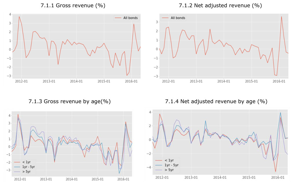
Note: Gross revenue is the monetary return expressed as a percentage of initial purchase monetary amount. Net adjusted revenue is gross revenue adjusted by funding cost and interest rate risk.
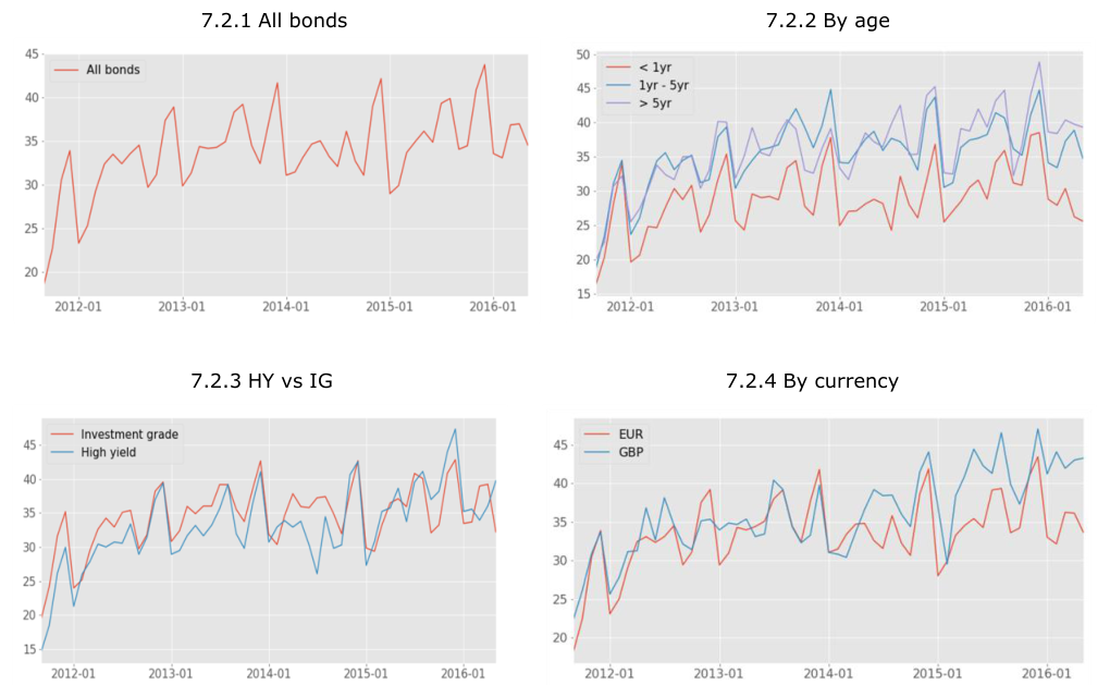
Note: Holding period is the average length of time between purchase and final sale (i.e., the completion of the round trip chain).
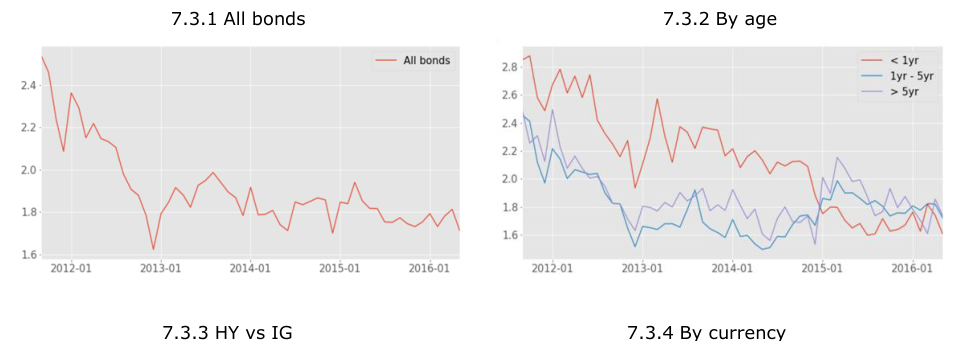
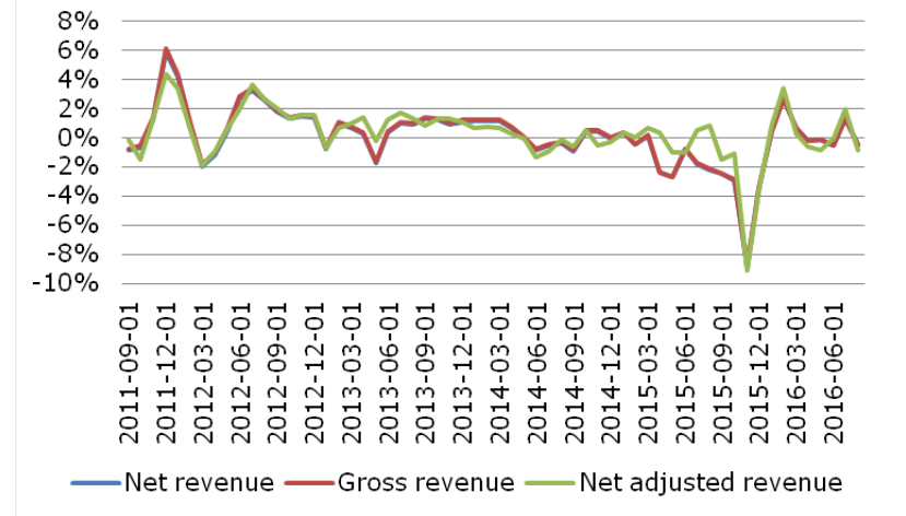
Note: This figure presents monthly averages of gross revenue, net revenue (gross revenue adjusted for funding cost) and net adjusted revenue (gross revenue adjusted for funding cost and interest rate risk).
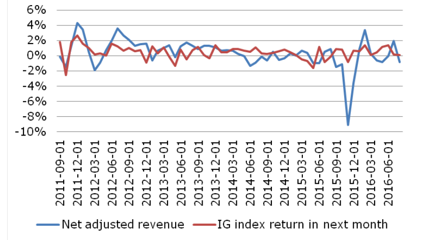
Note: IG index is Bloomberg investment grade EUR bond index. Monthly return is growth rate between the price at the beginning of the month and the end of the month.
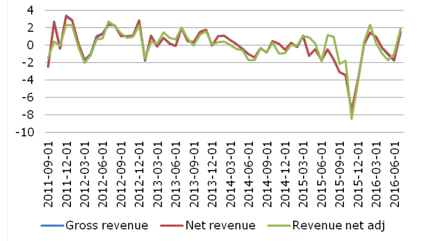
Note: Units are in percent. The data is shown for the period September 2011 to August 2016.
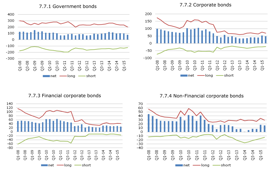
Note: The source is Grillet-Aubert et al. (2016). Variables are in Euro billion.
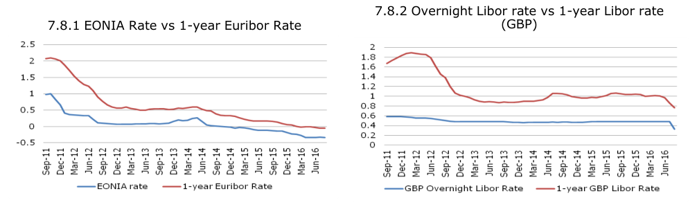
Note: The source is Bloomberg. Variables are in percent.
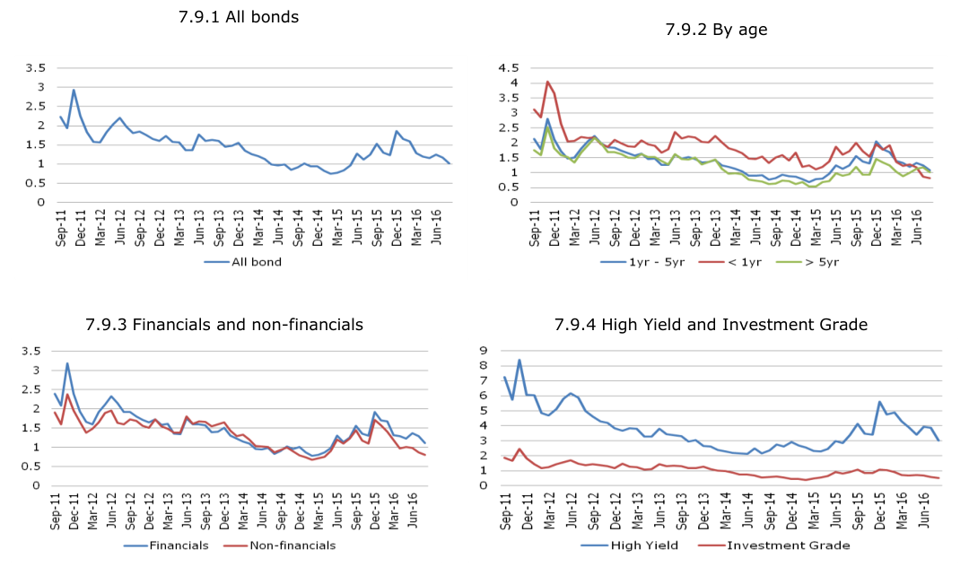
Note: The sources are FCA and Bloomberg. Variables are in percent.
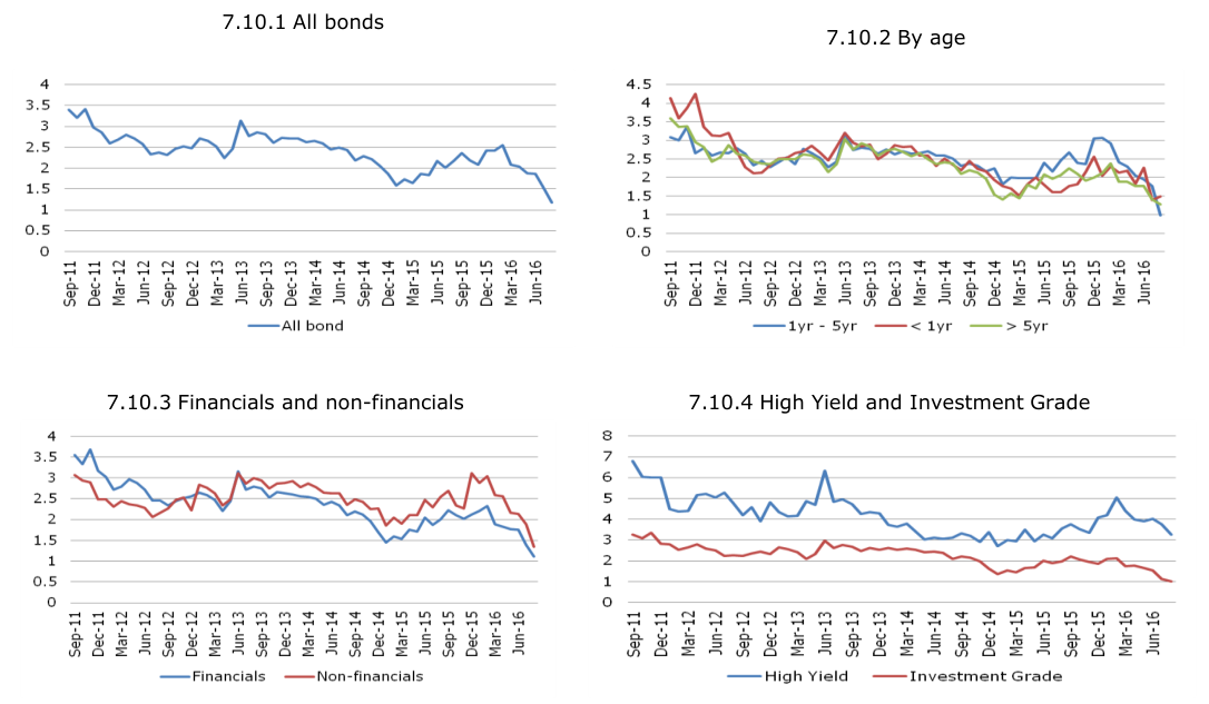
Note: The sources are FCA and Bloomberg. Variables are in percent.
| Panel a) Sample | period September | 2011 | to August | 2016 | |||
|---|---|---|---|---|---|---|---|
| Net | adjusted | ||||||
| Dependent Variable | Gross | revenue | Net | revenue | revenue | ||
| coef. | t-value | coef. | t-value | coef. | t-value | ||
| Constant | 0.20 | 0.90 | 0.12 | 0.52 | 0.35 | 1.55 | |
| IG index return | in next month | 0.99 | 3.92 | 0.99 | 3.90 | 0.64 | 2.50 |
| Time | -2.86 | -3.71 | -2.69 | -3.49 | -2.03 | -2.59 | |
| Panel b) Sample | period September | 2011 | to January | 2016 | |||
| Net | adjusted | ||||||
| Time Period | Gross | revenue | Net | revenue | revenue | ||
| Dependent Variable | coef. | t-value | coef. | t-value | coef. | t-value | |
| Constant | 0.15 | 0.68 | 0.06 | 0.27 | 0.31 | 1.34 | |
| IG index return | in next month | 0.88 | 3.44 | 0.87 | 3.42 | 0.54 | 2.05 |
| Time | -3.72 | -4.66 | -3.57 | -4.47 | -2.70 | -3.27 |
Note: This regression is based on monthly aggregated observations.
| Coeff. | t-stat. | Coeff. | t-stat. | Coeff. | t-stat. | |
|---|---|---|---|---|---|---|
| Constant | 0.384 | 2.903 | 0.447 | 3.304 | 0.447 | 3.346 |
| Time | -1.541 | -2.4 | -1.792 | -2.3 | -1.769 | -2.3 |
| IG Index Return | 0.988 | 10.9 | 1.085 | 10.9 | 1.104 | 11.3 |
| Aggregate Vol | - | - | -3.021 | -0.4 | -2.860 | -0.4 |
| Individual Vol | - | - | 0.013 | 0.5 | 0.016 | 0.7 |
| Log age | - | - | -0.063 | -1.5 | -0.058 | -1.4 |
| Log size | - | - | -0.091 | -1.3 | -0.080 | -1.1 |
| High yield | - | - | -0.092 | -0.8 | -0.103 | -0.8 |
| Financial | - | - | 0.146 | 1.2 | 0.151 | 1.3 |
| Upgrade | - | - | - | - | -0.041 | -0.2 |
| DownGrade | - | - | - | - | -1.310 | -4.7 |
| Number observations | 957,093 | - | 630,738 | - | 630,738 | - |
| Number months | 60 | - | 60 | - | 60 | - |
| Adjusted R-sq. | 0.08 | - | 0.10 | - | 0.10 | - |
| F-stat. | 68.11 | - | 23.49 | - | 44.41 | - |
| Panel b) Net adjusted revenue | ||||||
| Coeff. | t-stat. | Coeff. | t-stat. | Coeff. | t-stat. | |
| Constant | 0.628 | 3.605 | 0.662 | 3.631 | 0.662 | 3.652 |
| Time | -1.255 | -1.7 | -1.986 | -2.1 | -1.969 | -2.1 |
| IG Index Return | 0.665 | 6.9 | 0.740 | 6.2 | 0.748 | 6.3 |
| Aggregate Vol | - | - | -10.013 | -1.1 | -9.828 | -1.1 |
| Individual Vol | - | - | 0.051 | 2.8 | 0.053 | 2.9 |
| Log age | - | - | 0.004 | 0.1 | 0.007 | 0.2 |
| Log size | - | - | 0.065 | 1.1 | 0.072 | 1.1 |
| High yield | - | - | 0.154 | 1.4 | 0.147 | 1.3 |
| Financial | - | - | 0.095 | 0.9 | 0.098 | 0.9 |
| Upgrade | - | - | - | - | 0.218 | 0.8 |
| DownGrade | - | - | - | - | -0.649 | -2.8 |
| Number observations | 520,433 | - | 390,293 | - | 390,293 | - |
| Number months | 60 | - | 60 | - | 60 | - |
| Adjusted R-sq. | 0.04 | - | 0.08 | - | 0.08 | - |
| F-stat. | 26.17 | - | 9.62 | - | 10.14 | - |
Note: Estimated by Ordinary Least Squares with standard errors robust to time-specific clusters and serial correlations of 2 lagged periods (See Annex 6 for methodology). Unlike Table 7.1, regressions in Table 7.2 are based on individual round-trip observations. Individual Vol is the past 30 day Bloomberg mid-price volatility at beginning of the month. Aggregate Vol is the average of Individual Vol across bonds. Upgrade and Downgrade are dummy variables indicating rating transitions for a bond within a given month.
7.3 Regulatory pressures on market-making
Having presented different indicators or proxies for market-maker profitability in the last section, we now turn to a discussion of factors that may influence this profitability. (In the next section, we shall bring indicators and factors together and discuss how the factors may have influenced profitability.)
An obvious and important source of possible pressure on market-making profitability is regulatory change. Justified as a response to the financial crisis, regulatory change may have affected, in turn, dealer profitability, the availability of market-making services and ultimately market liquidity.
The ECB has conducted regular quarterly surveys on credit terms and conditions in euro-denominated securities financing and OTC derivatives markets (SESFOD). The surveys focus on euro-denominated instruments in securities financing and OTC derivatives markets. Survey participants are large banks and dealers active in targeted euro denominated markets.
In 2015 Q4 survey, more than 80% of respondents indicated that their market-making activities on high-quality financial corporate bonds, high-quality non-financial corporate bonds and high yield corporate bonds have decreased over the past year. Table 7.3 presents the main reasons cited by respondents for the decrease.
Most respondents to the 2016 Q4 survey also report decreased market-making activities in the past year. 83% of respondents reported a decrease in high-quality financial corporate bonds dealing, 63% reported reductions in high-quality nonfinancial corporate bonds and 67% respondents reported a decrease in high-yield corporate bond market-making. As observed in the 2015 Q4 survey, the main reasons for the decrease in activity are (in order) (i) Availability of balance sheet or capital at your institution, (ii) Compliance with current or expected changes in regulation and (iii) Profitability of market making activities. The 2016 Q4 survey also shows balanced numbers of respondents expecting their market-making activities will decrease or increase in 2017.
Figure 7.11 presents data on responses to a survey of European bond market-makers reported by Grillet-Aubert et al. (2016). The figure shows the percentage of survey respondents that identified different regulatory issues as discouraging market-making.
There are some problems in interpreting the survey responses as several of the issues may be viewed as overlapping. However, the primary conclusions one may draw are that the issue identified by the largest fraction of respondents as discouraging marketmaking is capital. This is closely followed by (i) the Basel 3 liquidity regulations, the Liquidity Coverage Ratio (LCR) and the Net Stable Funding Ratio (NSFR) and (ii) the transparency regime envisaged by MiFID 2.
In what follows, we will present calculations of capital costs and possible impacts of the liquidity regulation in order and compare their timing with the evolution of the indicators of profitability discussed above.
Tables 7.4 and 7.5 present information about the timing of changes in bank capital and liquidity rules associated with Basel 2.5 and 3. Banks were compliant with the Basel 2.5 rules by the end of 2010. The Leverage Ratio transition period began at the start of 2011 with a parallel run period commencing at the start of 2013.
Basel Committee proposals envisaged that the Liquidity Coverage Ratio (LCR) would be introduced on 1 January 2015. At that date, the minimum requirement would be set at 60%, rising in equal annual steps to 100% on 1st January, 2019.
The LCR transition periods in Europe and the US different slightly from those proposed by the Basel Committee. In Europe, the liquidity coverage has been introduced as follows: (a) 60 % of the LCR from 1 October 2015; (b) 70 % from 1st January 2016;
(c) 80 % as from 1st January, 2017; (d) 100% from 1st January, 2018.[85]
The US Final Rule requires covered companies to comply with a minimum LCR of 80% beginning on 1st January, 2015, 90% by 1st January, 2016, and 100% from 1st January, 2017. These transition periods are similar but shorter than those set forth out in the Basel 3 Revised Liquidity Framework.
The updated schedule NSFR in different jurisdictions is provided in BCBS (2017). In the US, proposals for the NSFR were issued in May 2016 and implementation is planned for January 2018. In the proposal for implementing the standard on the NSFR was adopted by the European Commission in November 2016. Again, implementation is planned for January 2018.
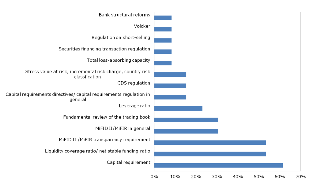
Note: The chart exhibits data from a survey of 13 large European, bond market-makers reported in Grillet-Aubert et al. (2016). Each bar shows the percentage of survey respondents that identified different regulatory issues as discouraging market-making.
| Possible reasons | for a | decrease | in | market making | activities First | Second | Third | Either first | ||
|---|---|---|---|---|---|---|---|---|---|---|
| (2015 Q4 survey) | reason | reason | reason | or second | or | |||||
| third reason | ||||||||||
| High-quality | financial | corporate | bonds | |||||||
| Willingness of | your institution | to take | on risk | 0 | 0 | 25 | 6 | |||
| Internal treasury | charges | for | funding | market-making | activities | 0 | 0 | 50 | 11 | |
| Availability of | balance | sheet | or capital | at your institution | 22 | 60 | 0 | 28 | ||
| Compliance | with current | or | expected | changes in regulation | 67 | 20 | 0 | 39 | ||
| Profitability of | market | making | activities | 11 | 20 | 25 | 17 | |||
| Total number | of answers | 9 | 5 | 4 | 18 | |||||
| High-quality | non-financial | corporate | bonds | |||||||
| Willingness of | your institution | to take | on risk | 0 | 0 | 25 | 6 | |||
| Internal treasury | charges | for | funding | market-making | activities | 0 | 0 | 50 | 12 | |
| Availability of | balance | sheet | or capital | at your institution | 13 | 40 | 0 | 18 | ||
| Availability of | hedging | instruments | 13 | 0 | 0 | 6 | ||||
| Compliance | with current | or | expected | changes in regulation | 63 | 20 | 0 | 35 | ||
| Profitability of | market | making | activities | 13 | 40 | 25 | 24 | |||
| Total number | of answers | 8 | 5 | 4 | 17 | |||||
| High-yield | corporate bonds | |||||||||
| Willingness of | your institution | to take | on risk | 0 | 25 | 0 | 9 | |||
| Internal treasury | charges | for | funding | market-making | activities | 0 | 0 | 33 | 9 | |
| Availability of | balance | sheet | or capital | at your institution | 25 | 25 | 0 | 18 | ||
| Compliance | with current | or | expected | changes in regulation | 25 | 25 | 33 | 27 | ||
| Growing | importance of | electronic trading | platforms | 0 | 25 | 0 | 9 | |||
| Profitability of | market | making | activities | 50 | 0 | 33 | 27 | |||
| Total number | of answers | 4 | 4 | 3 | 11 |
Note: The data source is European Central Bank Survey on credit terms and conditions in euro- denominated securities financing and OTC derivatives markets (SESFOD) 2015 Q4. The numbers are in percentages, except for the total number of answers. Other available but not chosen reasons in the questionnaire are: Competition from other banks, Competition from non-bank financial institutions, Constraints imposed by internal risk management (e.g. VaR limits), Role of high-frequency automated trading in making markets and other reasons.
| Basel rules | Timeline | ||||||
|---|---|---|---|---|---|---|---|
| BCBS 158: Revisions to the Basel II | |||||||
| market risk framework | Banks are | expected to | comply with the | revised | requirements by | 31 December | 2010 |
| The transition | period for | the leverage | ratio commenced | 1 January | 2011.The | ||
| transition | period comprises | a supervisory | monitoring | period and | a parallel | run | |
| period: The | supervisory | monitoring period | commenced | 1 January | 2011. | The | |
| supervisory | monitoring | process focused | on developing | templates | to track | the | |
| underlying | components | of the agreed | definitions | and resulting | ratio in a | consistent | |
| manner. The | parallel run | period commenced | 1 | January 2013 and | runs until | 1 January | |
| BCBS 270: Basel III leverage ratio | |||||||
| 2017. During | this period, | the leverage | ratio and its | components | are being | reported | |
| framework and disclosure | |||||||
| and tracked, | including its | behaviour | relative to the | risk-based | capital | requirement. | |
| requirements | |||||||
| The Committee | will | continue to test a | minimum | requirement of | 3% for | the leverage | |
| ratio during | the parallel | run period. The | public | disclosure | requirements | start on 1 | |
| January 2015. | Based on | the results of the | parallel | run period, any | final | adjustments | |
| to the definition | and | calibration of the | Basel III | leverage ratio | will be carried | out by | |
| 2017, with a | view to | migrating to a Pillar | 1 treatment | on 1 January | 2018 | based on | |
| appropriate | review and | calibration. |
| Rule | LCR phase-in | Source | |
|---|---|---|---|
| 01/01/2015 | 60% | ||
| 01/01/2016 | 70% | ||
| Basel | |||
| 01/01/2017 | 80% | BCBS 238 | |
| III | |||
| 01/01/2018 | 90% | ||
| 01/01/2019 | 100% | ||
| 01/10/2015 | 60% | ||
| Commission | |||
| 01/01/2016 | 70% | ||
| EU | (EU) 2015/61 | ||
| 01/01/2017 | 80% | ||
| Regulation | |||
| 01/01/2018 | 100% | ||
| 01/01/2015 | 80% | Liquidity | |
| US | 01/01/2016 | 90% | Risk Measurement |
| 01/01/2017 | 100% | Rule. Federal |
Note: The table shows the schedule for LCR compliance originally proposed by the Basel Committee and the schedules applied by the EU and the US Federal Reserve.
7.4 Quantifying capital pressure on market-making
To evaluate the effects of capital regulations on incentives to offer market-making services, we create a sample portfolio representative of the bonds contained in the FCA dataset. We then calculate what capital a bank that held such a portfolio would have to hold against the portfolio under the Basel 2.5 rules and examine how this varies over time.
To create a suitably representative portfolio, we estimated the joint distribution of bond turnover by rating, sector, country, currency and maturity. We then construct a portfolio made up of the 2,000 bonds which are most traded in the last year of the FCA data. As portfolio weights, we used shares based on the distribution by characteristics of the FCA data.[86]
To calculate capital, we used a set of simplified market risk capital models that provide a stylised representation of how a bank might derive Basel 2.5-consistent market risk capital, allowing for credit and interest rate risk.
The regulatory framework applicable for bank trading books evolved considerably with the adoption of Basel 2.5. Prior to the Crisis, banks were allowed to permit a variety of market risk VaR models with a holding period of ten days and a confidence level of 1%. The ten day holding period was usually implemented by employing a VaR model for 1-day returns and multiplying the capital by the square root of 10. Subject to supervisory permission, a bank may use an internal model to assign capital for specific risk.
Concerned about the accuracy of VaR models and the lack of attention to the liquidity of a bank’s trading book in the pre-crisis Basel 2 rules, regulators devised the changes in the Basel 2 framework referred to as Basel 2.5 and set out in Basel publications in July 2009 (see BCBS (2009a), BCBS (2009b) and (2009c)).
Under the July 2009 rules (see BCBS (2009b)), trading book capital charges for a bank using the internal models approach for market risk include a general market risk capital charge (inclusive of a specific risk capital charge) and a stressed Value-at-Risk charge. In addition, the bank must hold meet an additional Incremental Risk Charge (IRC) (see BCBS (2009c)) allowing for default risk in the trading book and designed to penalise illiquid positions.
The main components of our calculations are, therefore:
1. Portfolio VaR
2. Specific risk capital
3. Stress VaR
4. Incremental Risk Charge for default risk
We consider the exposure of the return on our representative portfolio to points on Treasury term structures and to credit spreads. It is necessary to calculate the bond’s market yield as it is not provided. Only vanilla bonds are chosen for the yield spread estimation exercise in that we exclude callable, puttable and convertible bonds. We also require that bonds have fixed payment frequency and that neither principal nor coupons be linked to indexes. For each ISIN, we take the median price of all transactions occurring during the last 5 or 8 working days of each month. To calculate the market yield, we calculate the accrued interest based on the bond's payment structure information as well as its day count convention. Adding up the price and the accrued interest, we derive a dirty price. A bond's yield is found using the Newton method by equating the discounted value of the bond’s cash flows to its dirty price.
We collect time series data on factors representing returns on pure discount bonds at different points on the term structures of multiple currencies. These are denoted . We also collect time series of credit spreads by rating and maturity, denoted . Given the current portfolio breakdown by maturity and rating, we calculate the impact on portfolio values of the interest rate factors (the weights are denoted . and the credit risk factors (the weights are denoted
associated with a given bucket so that their total par equals the adjusted weight for that bucket. The total par values of the 2,000 bonds then sums to unity.
To estimate , we then construct a vector of the portfolio value changes consisting of on each date using formula (7.1):
(7.1)
The length of is . An estimate for is the 99% quantile of based on daily data scaled up to ten days. We repeat this exercise for each date , and thereby obtain a time series of portfolio s. We use the rules set out in Table 7.6 to calculate the specific capital risk charge.
Under the Basel 2.5 rules, a bank must calculate a ‘stressed value-at-risk’ measure similar to the standard VaR calculation but based on a calibration based on historical data from a continuous 12-month period of significant financial stress relevant to the bank’s portfolio. As an example, for many portfolios, a 12-month period relating to significant losses in 2007/2008 would adequately reflect a period of such stress; although other periods relevant to the current portfolio must be considered by the bank.
Combining the VaR and the Stress VaR, a bank obtains its trading book capital requirement as follows.
(7.2)
Here, is the previous day’s Value-at-Risk, is the average of the daily value-at-risk of preceding 60 business days, the multiplier is set to 3 and is the stressed Value-at-Risk.
The final component of the trading book capital charge is the Incremental Risk Charge (IRC). This is based on an estimate of the default and migration risks of unsecuritised credit products over a one-year capital horizon at a 99.9% confidence level, taking into account the liquidity horizons of individual positions or sets of positions.
We estimate the IRC using a Monte Carlo simulation simulated up to a one-year horizon broken into four quarterly time steps. Any position that experiences default or rating migration during the quarterly periods is rebalanced at the end of the period. The rebalancing is implemented by reinvesting the available funds in assets with the same credit characteristics (initial rating and maturity) at the end of quarterly horizon.
| Table 7.6: | Specific risk | capital | charges | for | issuer | risk | |||
|---|---|---|---|---|---|---|---|---|---|
| External | |||||||||
| Categories | credit | Specific risk capital | charge | ||||||
| AAA to AA- | 0% | ||||||||
| A+ to BBB- | 0.25% (residual | term | to | final | maturity | 6 months | or less) | ||
| 1% (residual term | to | final | maturity | greater than 6 | and | up to and | |||
| Government | 1.60% (residual | term | to | final | maturity | exceeding | 24 | months) | |
| BB+ to B- | 8% | ||||||||
| Below B- | 12% | ||||||||
| Unrated | 8% | ||||||||
| 0.25% (residual | term | to | final | maturity | 6 months | or less) | |||
| Qualifying | 1% (residual term | to | final | maturity | greater than 6 | and | up to and | ||
| 1.60% (residual | term | to | final | maturity | exceeding | 24 | months) | ||
| Similar to credit | risk charges | under | the | standardised | approach of | this | Framework, | ||
| BB+ to BB- | 8% | ||||||||
| Other | |||||||||
| Below BB- | 12% | ||||||||
| Unrated | 8% |
7.5 Capital calculations for a market-maker portfolio
Here, we present the results of our capital calculations for the representative portfolio based on FCA data. Figure 7.12 shows the evolution of the 10-day VaR.
Figure 7.13 shows the evolution of the capital charge based on the equation (7.2) including the influence of the 60-day lookback period VaR and the Stress VaR. Figure 7.13 also shows the Incremental Risk Charge (IRC), the Specific Risk Charge and total capital. The IRC is calculated using by applying a Monte Carlo model to the representative portfolio made up of 2,000 bonds from the FCA dataset using statistical inputs estimated for each time period. The IRC capital is broadly flat although its evolution shares some of the features of the VaR/SVaR because the factor correlations that it uses as inputs also rise in the crisis period.
What lessons do we learn from these capital calculations? The total capital is high with the sum of VaR/Stress VaR, Specific Risk and IRC capital being around 8-9% across the period considered. The total capital shows some small fluctuations driven by changes in spreads and their volatilities and covariances, but overall the results are very risk insensitive. This reflects the “capital flattening” effect of the use of Stress VaR and the fact that the IRC is based on a long-run and relatively slow moving calibration.
It is often argued that high trading book capital charges have discouraged banks from making markets. The results shown here for a stylised portfolio suggest that capital has not been a driver of the reduction in inventories that we see in the ESRB Grillet- Aubert et al. (2016) study. The Basel 2.5 changes came in earlier and appear quite risk insensitive and, hence, stable over time.
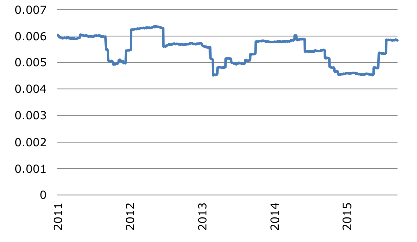
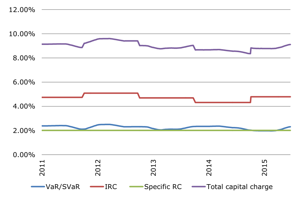
7.6 Pressure of liquidity rules on market-making
We now turn to an examination of the impact of liquidity rules on market-making. Liquidity rules represent restrictions across broad swathes of a bank’s asset base (in the case of the LCR) or across the entire balance sheet (in the case of the NSFR). It is therefore not straightforward to calculate their impact as a quasi-tax on activity as one may for capital.
In this section, we focus on the efforts that banks made in the period following 2010 to become compliant with the liquidity ratios. In the case of the LCR, a formal process of increasing compliance was envisaged by regulators with successively higher trigger levels for the ratio that banks had to exceed. But in fact banks were pushed by regulators and the market to become LCR and NSFR compliant much earlier than the formal rules. From early on in the implementation process, the presentations that banks prepare each quarter for bank equity analysts contained “FLB3” (“Front Loaded Basel 3”) figures showing how close to complying with the liquidity requirements banks had become.
For this reason, the pace with which banks struggled to become compliant with LCR and NSFR is easier to observe in the Quantitative Impact Study (QIS) publications of regulators. Specifically for Europe, the European Banking Authority (EBA) published a sequence of studies showing the progress banks made with their liquidity ratio compliance. The results of these QIS studies are summarised in Figures 7.14 and 7.15.
Figure 7.14 shows how the LCR ratio, averaged across bank, evolved from June 2011 to June 2016 using six-monthly time steps. The averages shown distinguish between large and small banks (“Group 1” and “Group 2” banks).
The key point to note in Figure 7.14 is the time periods in which European banks increased most significantly their LCR. For large banks, the biggest compliance effort was over 2012 when the average LCR went from 66% to 109%. In 2014, a second rise in the large bank average from 114% to 125% occurs. These changes, particularly the first, presumably required large shifts in European bank balance sheets.
Figure 7.15 shows the average NSFRs of European banks again for the period June 2011 to June 2016. The NSFR compliance effort made by European banks appears smoother than for the LCR. The six monthly changes are generally small. The largest increases for large banks are 4% in the second half of 2011, and 6% in the second half of 2013.
Another way to look at European banks’ efforts to comply with the Basel 3 liquidity ratio requirements is to look at the aggregate shortfall across European banks in High Quality Liquid Assets (HQLA), the numerator in the LCR) or the aggregate shortfall in Available Stable Funding (ASF), the numerator of the NSFR. These shortfalls are shown, for large and small banks, in Figures 7.16 and 7.17. The substantial effort that European banks made to comply with the LCR is evident in the sharp declines in the aggregate shortfalls in the two halves of 2012. Smaller banks began their compliance efforts slightly earlier with the biggest decline being in the second half of 2011.
The aggregate bank shortfall for NSFR compliance is shown in Figure 7.17. As with the average ratios shown in Figure 7.15, it appears that the sharpest correction in the shortfalls occurred in the second half of 2011 and the second half of 2013. As remarked earlier, NSFR compliance represented a more gradual process by European banks.
How might one expect the effort to become compliant with LCR and NSFR funding ratios to have affected market-making operations? As explained above, compliance with liquidity ratios has been mainly achieved by banks through changes in internal funding rates employed by treasury/ALM operations. Reportedly, some major European banks shifted their bond dealing operations from overnight to 1-year funding during the period 2013-15. At the same time, treasury operations employed managerial adjustments to funding rates, charging market-making operations supplementary spreads over the bank’s true external cost of funds.
Figure 7.18 provides illustrative calculations of what these changes in internal funding costs may have implied for a particular market-making operation. Panel a) shows results for EUR-denominated bonds. The green line shows the carry spread assuming overnight funding. Developments in this spread reflected the general interest rate environment that was itself significantly influenced by central bank actions. From December 2012, over a period of 12 months, we suppose that the bank progressively requires market-makers to use 1-year rather than overnight funding. While this evolution occurred through internal policy changes of commercial banks, it also probably anticipated the expectations of regulators. This second effect reduces the carry spread to the blue line shown in the figure.
Furthermore, it is assumed that the bank progressively moves from a 20 basis point managerial adjustment to the funding cost of dealer inventory to a 30 basis point adjustment again over a two year period. The result of these two funding policy changes is the red line that appears in panel a) of 7.19.
As one can observe, the carry spread is lowest in early 2015 for both EUR- and GBP denominated bonds. The most recent level of spreads is only slightly higher than that low.
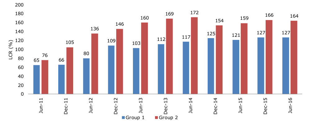
Note: The source is EBA QIS data (June 2016). Variables are in percent.
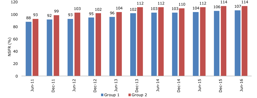
Note: The source is EBA QIS data (June 2016). Variables are in percent.
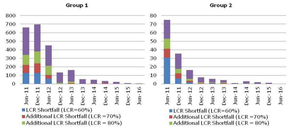
Note: The source is EBA QIS data (June 2016).
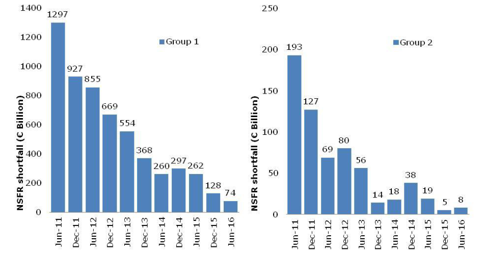
Note: The source is EBA QIS data (June 2016).
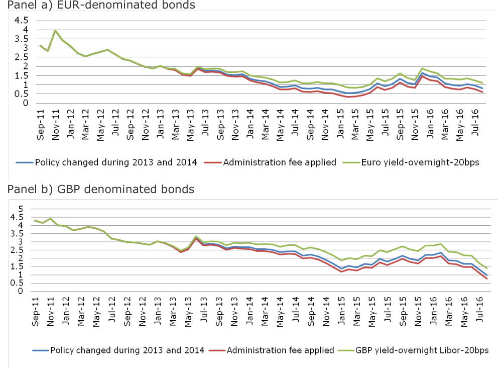
Note: Source include the FCA data and Bloomberg. Variables are in percent. We assume the administration fee 0.5% to 1% and growth generally between 2013 January and 2014 December.
7.7 Timing of shocks to market-maker profitability
Here, we turn to the lessons one may draw from the above discussion. We are interested in pressure on market-maker profitability because of the evidence presented in Section 3 that quantity-based indicators of liquidity appear to deteriorate over the period 2011-2016 and that price-based indicators, despite improving in the aftermath of the 2011 crisis, appear to deteriorate after 2014. When the price-based indicators are adjusted for risk (by conditioning on volatility), their improvement after the crisis appears less marked and a worsening seems to occur after 2013.
It is natural to consider the pressures on market-making profitability that we have discussed in this section as candidates for explaining these dynamics in liquidity indicators. Key to discussing this is clarity about the timing of the effects and the possible causes.
Figure 7.19 summarises some of the findings of this section as regards timing. Among the proxies for market-maker profitability that we consider, dealer inventories declined sharply in 2011 and 2012. Carry spreads, on the other hand, drifted down over the period 2012 to 2015. How do these developments compare to regulatory changes?
Figure 7.19: Time line of liquidity developments
From the EBA QIS data, it appears that European banks exerted themselves to be compliant with the Basel 3 liquidity rules between 2011 and 2014. On the other hand, the quantity-based liquidity indicators deteriorated gradually over the whole period 2010 to 2016 and the price-based indicators worsened only from 2014 onwards (or from 2013 when adjusted for risk).
It is difficult from these events to see a completely clear picture in which particular events generated unambiguous outcomes for corporate bond market liquidity. As mentioned above, corporate bond market-making is a flow business in which participants’ perceptions of changes in viability of activities takes time to accumulate. In this case, the cumulative impact of different changes in the regulatory and market environment could impair liquidity in a gradual way.
To conclude, this section presents an analysis of drivers of market-maker profitability. Directly observing this profitability is challenging but we identify and calculate a set of proxy variables including round-trip returns, inventories and carry yields net of funding costs. In each case, we bring data to bear, calculating the time profile of these indicators over the last few years. We examine possible influences on profitability including most notably regulatory capital and liquidity rules. The timing of the adoption of new regulations does not coincide exactly with obvious developments in our profitability indicators but one can make a case for the fact that the adoption of liquidity rules had an impact on dealer inventories. Pressure on the underlying returns from market-making appear to have drifted down over a number of years, reducing the degree to which dealers could absorb the costs of new regulations without a contraction in activity levels.
8. Dealer Inventories and EU Corporate Bonds Spreads
Summary of findings:
1. Earlier sections of this report have been concerned with the state and determinants of liquidity in the European Corporate bond market. This section focuses instead on the possible implications of liquidity on the pricing of corporate debt.
2. We calculate yield spreads on corporate bonds using the Bloomberg and FCA data described in earlier sections. The FCA data extends only slightly before the date when dealers in Europe reduced their inventories whereas the Bloomberg data is available over a longer period.
3. Using the Bloomberg data, we study how yield spreads have been affected by a range of cross sectional and time series factors. To examine spreads holding credit quality and risk constant, we regress yield spreads on ratings dummies and measures of volatility (ISIN-level and aggregate). By also including such time series variables as dealer inventories, we are able to measure the impact of changes in inventories corporate bond pricing.
4. The analysis should be regarded as descriptive of the data rather than a rigorous demonstration of causal effects. Our findings are consistent with a statistically and economically significant association between declines in dealer inventories and increases in credit spreads.
8.1 Introduction
There has been much recent comment on the declining levels of dealer inventories in major bond markets and the possible implications for liquidity. Adrian et al. (2015) comment on the decline in inventories but dispute that this has negatively affected liquidity. Himmelberg and Henson (2015) provide a counter view from an industry perspective.
Although disputed by Adrian et al. (2015), most would expect declines in dealer inventory to boost EU corporate bond credit spreads. While there may be a direct demand effect on corporate bond prices and hence yields, most of the impact is likely to reflect the increased transactions costs that bond holders will face if dealers curtail their market making activities.
Estimating the magnitude of the effect requires that one calculate (i) the impact of dealer inventories on transactions costs and (ii) the degree to which higher current transactions costs feed through into bond price discounts or, equivalently, credit spreads.
In general, corporate bond yields comprise multiple components including the Treasury yield for the same maturity, expected credit losses (inclusive of a risk premium), tax effects and spreads to compensate the holder against the current or possible future illiquidity of the bond.
The illiquidity spread reflects not just current transactions costs multiplied by expected frequency of future trading in a given position. Even if the bid-offer spread is currently narrow, the bond holder may anticipate a possible future need to sell and this sale may coincide with stressed market conditions in which trading costs are high. Furthermore, the holder may themselves anticipate possibly being in financial difficulties in this stress situation in which case they will add a hefty risk premium to their current forecast of future trading costs.
Various papers have attempted to decompose credit spreads into different components in order to gauge the impact of illiquidity discounts on bond prices. A notable such study is Dick-Nielsen, Feldhütter and Lando (2012). These authors regress yield spreads to the swap rate on proxies for liquidity and control variables and then estimate the liquidity premium by the contribution to spreads of the liquidity indicators multiplied by their regression coefficient. Aquilina and Suntheim (2016) use the same approach as Dick-Nielsen et al. (2012).
We will employ comparable techniques including dealer inventory levels as a time series determinant of spreads along with other time series and cross-sectional bond and issuer characteristics.
We will use the dealer inventory data collected by the European Systemic Risk Board (ESRB) study discussed in Section 2, Grillet-Aubert et al. (2016), and presented in
Figure 2.11. These data are based on a survey of 13 large European market-makers.
Inspection of Figure 2.11 suggests that European corporate bond dealer inventories experienced a regime change dropping sharply in late 2011 or early 2012. Before and after this time, inventories, although they fluctuate somewhat, are broadly constant. Our analysis is in the spirit of an event study, therefore. We effectively examine whether, other factors being equal, corporate bond spreads were noticeably high after the sharp drop in inventories compared with the period before.
In performing the analysis, we condition on various cross-sectional influences. To this effect, we include dummies for ratings and a measure of bond age. A crucial additional influence on which we want to condition is the risk of the bonds in question. To allow for risk, we include in the regression bond-specific and market wide volatility measures (as we did in the regressions reported in Section 3).
The reason why conditioning on risk is crucial is that, following the crisis, spreads clearly fell. By conditioning on risk (proxied by volatility), we pose the question did spreads fall by less than one would expect given what happened to risk?
It is true that a quasi “event study” or the type presented here cannot provide conclusive evidence that inventory changes caused an apparently high level of spreads. The problem is that relatively little evidence in the time series dimension is available. But, it remains interesting to explore the issue and to calibrate the magnitude of the effect that the analysis suggests.
8.2 Data on Yield Spreads
To construct yield spreads, we calculate the price of a notional, default-free bond having the same contractual cash-flows as the bond in question. We then take the difference between the yield on the defaultable corporate bond and the yield on the notional default free security.
To obtain the price of the notional bond, one must discount contractual cash flows using “default free” rates. Dick-Nielsen et al. (2012) and Aquilina and Suntheim (2016) calculate yield spreads employing as “default free” rates swap yields. In our analysis, we prefer to employ Treasury pure discount bond yields. (In fact, Dick-Nielsen et al. (2012), use both swap yields and Treasury yields as the basis for calculating yield spreads but only report results in detail for the former.)
Our preference for Treasury yields is based on the fact that the period we are studying includes a banking crisis. Swaps are generally collateralised and, hence, close to default free. But, the rate on the fixed leg of a swap inherits a credit spread since the floating leg is indexed to a non-collateralised, defaultable floating rate. In a banking crisis, swap yields (just like interbank deposit rates such as Libor) may substantially exceed default free rates. We examined AAA and AA corporate bond yields for the period covered by this study and found that they were less than swap yields for some periods.[87]
Using the approach described above, we construct yield spreads for two bond datasets: (i) the bonds contained in the FCA dataset and (ii) the bonds in the Bloomberg dataset. Below, we focus only on results obtained using the Bloomberg data. The reason is that the FCA data starts no more than three months before the step change in inventories apparent in Figure 2.11. Basing a ‘quasi’ event study on a dataset in which only a few observations are available for the period before the event appears ill-advised. In contrast, the Bloomberg bond data stretches back further in time to well before the start of the dealer inventory data that we employ.
Only vanilla bonds are chosen for the yield spread estimation exercise in that we exclude callable, puttable and convertible bonds. We also require that bonds have fixed payment frequency and that neither principal nor coupons be linked to indexes. For the Bloomberg data, we take daily bid price and bid yield data from the Bloomberg BGN data source. For each month and ISIN, the median bond price and its corresponding yield are picked from the observations on the last 5 working days of the month (or 8 working days if the month is December). Each bond's future cash flow is then constructed from its date of price, coupon rate, coupon frequency and maturity date.[88]
Figure 8.1 shows the yield spread data for the Bloomberg bond data. For each month, top 0.5% and bottom 0.5% yield spread data is winsorised. It is interesting to observe that the yield spread data shows much more sensitivity to the first phase of the financial crisis following the 2008 collapse of Lehman Brothers than the bid-ask spreads presented in Figure 3.13. In other words, the riskiness of bonds rose in the early phase of the crisis without a major increase in trading costs.
Figure 8.1: Yield spreads over Treasury rates - Bloomberg non-financial bonds
Figure 8.2: Yield spreads over Treasury rates - FCA data
Figure 8.1.1 suggests that the term structure of spreads was hump shaped in the early crisis phase in that short and long yields were relatively low. In the 2011-12 phase of the crisis the term structure of spreads is inverted with short maturities exhibiting higher spreads. Note that, towards the end of the sample period, yield spreads rise until the ECB asset purchase program leads them to fall back to low levels.
Figure 8.1.2 shows that yield spreads for the Netherlands were highest in the first phase of the crisis whereas, in the second phase, Italian bond spreads were highest. Figure 8.1.3 shows that USD-denominated bonds reached very high peaks in 2008-9. In 2011-12, there is little difference between the yields for different currency denominations. Figure 8.1.4 shows that, for both crisis periods, financial issuer yields exceeded those for non-financial issuers. A strong issue size effect is visible in yield spreads as shown by Figure 8.1.5.
When bonds are bucketed by past volatility, yield spreads appear the same in phase 1 of the crisis but in 2011-12, the bucketing flattens out the rise in yield spreads. This shows that the rise in spreads reflected the differing riskiness of the bonds and that conditioning on this would attenuate the spike.
Figure 8.2 shows the equivalent to 8.1 but for the FCA yield spreads. The sample period is shorter but one may observe some similar patterns, including a downward sloping credit spread term structure in the 2011-12 period (8.2.1), high Italian bond spreads (8.2.2), relatively high USD-denominated bond spreads (8.2.3), high spreads for financials versus non-financials (8.2.4), a strong issue size effect (8.2.5), a smoothing out of the spikes in spreads with volatility bucketing (8.2.6) and consistent age (8.2.7) and rating effects (8.2.8). It seems that the same patterns are evident in both Bloomberg and FCA yield spreads.
8.3 Potential explanatory variables for yield spreads
The approach we take is to perform a panel regression of monthly observations of Bloomberg yield spreads at the ISIN level on a combination of cross sectional and time series drivers.
We wish to allow for credit quality. In their yield spread regressions, Dick-Nielsen et al.
(2012) and Aquilina and Suntheim (2016) employ issuer-specific financial ratios and ratings. (Dick-Nielsen et al. (2012) condition on ratings broken down by specific ratings grades whereas Aquilina and Suntheim (2016) include a dummy for Investment Grade versus High Yield.)
One may be concerned that the credit quality implications of financial ratios vary across sector and may not provide a fully reliable measure of credit risk in the absence of detailed and complex allowances for the nature of the firm’s activities. We, therefore, rely on ratings alone to condition on credit quality. Ratings themselves may be criticised as the basis for credit quality adjustments. Another drawback is that some bonds may not be rated.
We primarily use S&P ratings but if these are not available we successively use a Moody’s rating. If the latter cannot be obtained we use Fitch and ultimately DBRS ratings. (We presume that all can be mapped between each other on the usual consistent scale.) As we argued above, we believe that use of issuer financial ratios to condition on credit quality is ill-advised as the interpretation of these ratios varies so dramatically across sectors, reflecting differing business models. As well as ratings, we also include maturity and currency dummies as cross-sectional issue-specific determinants of yield spreads.
Figure 8.3: Time series variables that could explain yield spreads
Ratings (and indeed financial ratios) are slow moving indicators of credit quality in part reflecting the fact that the ratings agencies follow through the cycle approaches to credit evaluation. It is, therefore, also important to condition on risk more directly. With this aim, we include as right hand side variables in the yield spread regression (i) a measure of bond specific volatility calculated using the previous 30 days of return data, and (ii) an equally weighted index of such volatilities as a market-wide risk indicator.[89]
Having conditioned on ratings, maturity, currency and volatility, we investigate the effect on spreads of time series variables including market-maker inventories. To understand the role that time series variables may play, we present several plots in
Figure 8.3. The plots include the ESRB inventory data for financial and non-financial bonds, the 1-year and 5-year swap rates. The latter two series may be seen as reflecting the interest rate environment.
8.4 Regression analysis of yield spreads
Tables 8.1 and 8.2 present the results of our regression analysis. Table 8.1 shows regressions of Bloomberg data for non-financial yield spreads on cross sectional and time series variables. Three regressions are presented excluding and including the 1 year swap rate and the slope from 1 to 5 year swap rates.
The coefficients on the ratings variables consistently exhibit values that are monotonically decreasing in the rating grade except for the CCC dummy. The coefficients on maturity are insignificant reflecting the fact that the slope of the credit term structure has changed over the sample period (downward sloping in some crisis periods and upward sloping in others).
The currency dummies are consistent with expectations (after inspection of the plots above) in that they suggest USD-denominated bond yield more than those in GBP or EUR. The volatility variables are highly significant, particularly the individual volatility (which of course varies over time and across ISINs). Both have the expected signs.
Turning to the inventory data, both long and short inventory positions exhibit consistently statistically significant coefficients. In both cases, signs are as intuitively expected in that higher positive inventories imply lower yield spreads. Negative inventories are included as negative values and hence one may expect to find a positive coefficient if greater scope for shorting bonds leads to higher liquidity and lower yields. The inclusion of the 1 year swap rate and the swap rate slope variable does not substantially affect the coefficients on inventories. Nor does the inclusion of these additional variables affect the R-square statistics which equal 48%.
The third regression for which results are shown in Table 8.1 replaces the inventory variables with a dummy variable equalling unity before July 2011 and zero otherwise. This regression treats the drop in inventories as an event and allows one to examine whether a significant change in the level of spreads is associated with the contraction of dealing activity reflected in the drop. The inventory drop dummy has a significant parameter with a magnitude that appears economically significant (37 basis points).
Table 8.2 presents regression results for Bloomberg data yield spreads for financial bonds. Many of the observations about the non-financial yield spread results remain true. In this case, the maturity variable is significantly negative, however, reflecting the greater importance of crisis period inverted credit term structures for bank bonds. The volatility index has a negative sign but is not at all significant statistically.
Some of the variables appear surprising until one recalls that the yield spreads are for financial bonds in the most part issued by banks. The swap yield has a negative coefficient (unlike for non-financial yield spreads for which the coefficient was positive). This is reasonable as lower interest rates impair bank profitability and, hence, boost yield spreads for bank bonds.
The coefficients for long inventories are negative as one might expect. Higher inventories boost liquidity and hence reduce yields. The coefficient for short inventories is also negative, however. This appears counter-intuitive but there are mechanisms other than liquidity driving the relationship between short bank bond positions and bank credit quality. If banks short bank bonds in order to hedge themselves against deterioration in the credit quality of other banks, one will observe that larger short inventories will coincide with higher bank bond yield spreads. The inventory dummy regression (for which the results are shown in columns 6 and 7 of Table 8.1) again exhibits a statistically significant parameter with a counter-intuitive sign. Once again, we would interpret this as reflecting influences on bank bond spreads other than liquidity.
| Coeff | t-stat | Coeff | t-stat | Coeff | t-stat | |
|---|---|---|---|---|---|---|
| Constant | 1.91 | 44.84 | 1.91 | 45.43 | 1.91 | 39.66 |
| AA dummy | 0.23 | 5.28 | 0.24 | 5.24 | 0.28 | 6.21 |
| A dummy | 0.63 | 15.36 | 0.63 | 15.64 | 0.66 | 14.79 |
| BBB dummy | 1.27 | 16.58 | 1.27 | 16.62 | 1.29 | 15.56 |
| BB dummy | 3.17 | 21.83 | 3.17 | 21.97 | 3.16 | 21.90 |
| B dummy | 5.97 | 16.60 | 5.96 | 16.73 | 6.01 | 16.20 |
| CCC dummy | 4.71 | 2.70 | 4.72 | 2.71 | 4.59 | 2.62 |
| NR dummy | 1.61 | 22.50 | 1.62 | 24.12 | 1.65 | 22.03 |
| Maturity | 0.00 | -0.55 | 0.00 | -0.57 | 0.00 | -0.34 |
| GBP-denom | -0.27 | -5.33 | -0.32 | -4.66 | -0.28 | -4.05 |
| EUR-denom | -0.32 | -5.28 | -0.36 | -6.01 | -0.31 | -6.12 |
| Long inventory | -0.01 | -3.06 | -0.02 | -2.07 | - | - |
| Short inventory | 0.03 | 5.38 | 0.03 | 5.49 | - | - |
| Inventory dummy | - | - | - | - | -0.37 | -2.63 |
| Volatility | 0.10 | 8.26 | 0.10 | 8.27 | 0.10 | 8.25 |
| Volatility index | 6.99 | 5.21 | 6.63 | 4.50 | 10.97 | 5.71 |
| 1-year rate | - | - | 0.02 | 0.29 | 0.06 | 0.78 |
| Yield curve slope | - | - | -0.07 | -0.79 | 0.02 | 0.26 |
| Number observations | 35,055 | - | 35,055 | - | 35,055 | - |
| Adjusted R-sq | 0.48 | - | 0.48 | - | 0.47 | - |
| F-stat | 285.24 | - | 294.47 | - | 404.84 | - |
| P (F-stat) | 0.00 | - | 0.00 | - | 0.00 | - |
Note: Estimated by Ordinary Least Squares with standard errors robust to time- specific clusters and serial correlations of 2 lagged periods (See Annex 6 for methodology). Inventory dummy equals unity before 07/2011 and zero otherwise.
| Coeff | t-stat | Coeff | t-stat | Coeff | t-stat | |
|---|---|---|---|---|---|---|
| Constant | 2.27 | 34.88 | 2.27 | 35.62 | 2.27 | 28.08 |
| AA dummy | 0.37 | 4.85 | 0.36 | 4.67 | 0.35 | 4.38 |
| A dummy | 0.75 | 9.25 | 0.73 | 8.97 | 0.72 | 8.82 |
| BBB dummy | 1.38 | 12.50 | 1.37 | 12.38 | 1.35 | 12.32 |
| BB dummy | 3.01 | 10.88 | 3.00 | 10.93 | 2.98 | 10.82 |
| B dummy | 4.46 | 4.96 | 4.45 | 4.98 | 4.38 | 4.88 |
| CCC dummy | 13.25 | 3.75 | 13.23 | 3.74 | 13.13 | 3.72 |
| NR dummy | 1.27 | 13.78 | 1.26 | 13.25 | 1.28 | 12.76 |
| Maturity | -0.11 | -5.39 | -0.11 | -5.34 | -0.11 | -5.27 |
| GBP-denom | -0.12 | -1.83 | 0.02 | 0.17 | -0.19 | -2.42 |
| EUR-denom | -0.38 | -3.58 | -0.28 | -2.50 | -0.48 | -4.81 |
| Long inventory | -0.03 | -3.05 | -0.03 | -3.83 | - | - |
| Short inventory | -0.06 | -3.91 | -0.08 | -5.22 | - | - |
| Inventory dummy | - | - | - | - | 0.51 | 2.44 |
| Volatility | 0.30 | 7.30 | 0.30 | 7.28 | 0.30 | 7.30 |
| Volatility index | -1.24 | -0.37 | -0.54 | -0.15 | -2.34 | -0.65 |
| 1-year rate | - | - | -0.08 | -0.82 | -0.07 | -0.79 |
| Yield curve slope | - | - | 0.12 | 1.03 | -0.21 | -2.03 |
| Number observations | 71,811 | - | 71,811 | - | 71,811 | - |
| Adjusted R-sq | 0.46 | - | 0.46 | - | 0.46 | - |
| F-stat | 122.30 | - | 175.45 | - | 209.44 | - |
| P (F-stat) | 0.00 | - | 0.00 | - | 0.00 | - |
Note: Estimated by Ordinary Least Squares with standard errors robust to time- specific clusters and serial correlations of 2 lagged periods (See Annex 6 for methodology). Inventory dummy equals unity before 01/2012 and equals zero otherwise.
8.5 Implications of the analysis
Regression analysis of this kind must necessarily be treated with caution. We are aware of the limited time series information offered by our dataset. One could, no doubt, include other time series variables and find combinations that vitiate the significance of the inventory variables included in these regressions. Hence, the results presented here should be viewed as suggestive rather than as a fully convincing scientific demonstration of the impact of inventory volumes on bond yield spreads.
Despite the above cautious comments, it is interesting to calculate the economic magnitude of the inventory effects that we have estimated using the regression analysis. Table 8.3 presents calculations of the impact on yield spreads of inventory changes.
The calculations presented in Table 8.3 show the economic significance of the effects estimated in the regression analysis. Declines in long inventories of €10 to €30 billion imply increases in non-financial yield spreads of between 15 and 45 basis points according to the Bloomberg data regressions. The actual drop in long inventories in the period from Q2 2011 to Q2 2012 (the period of steepest decline for long non-financial inventories) was €25 billion. Declines in short inventories also generate large increases in yield spreads according to the regression results. The Bloomberg data results actually suggest the effects are larger than for equal declines in long inventories.
To conclude, in most of this study, we have focussed on the drivers of liquidity in the European corporate bond market. In this section, we have considered the implications of liquidity for the costs of funding for bond issuers. We present statistical analysis of the effects of changes in market-maker inventories on yield spreads in European corporate bonds. Conditioning on cross sectional variables and some time series influences like volatility, we find that changes in dealer inventories have marked impacts on the cost of funds to bond issuers. The sizeable magnitude of the effects are striking and the calculations are consistent with the notion that illiquidity implies costs to the real economy via its effects on pricing in the primary market.
| 10 | 0.15 |
|---|---|
| 20 | 0.30 |
| 30 | 0.45 |
| inventories (€billion) | |
| 10 | 0.28 |
| 20 | 0.56 |
| 30 | 0.84 |
Note: Y2011-Y2012 marks the time from 2011 Q2 to 2012 Q2 when non-financial bonds' long inventories dropped by €25 billion.
9. Conclusions
This report presents the findings of a study of drivers of liquidity in the European corporate bond market. We also examine the growing role of Electronic Trading Platforms (ETPs) and the implications for liquidity of pre- and post-trade transparency rules. Finally, we study influences on dealer profitability and the impact of changes in dealer inventories on corporate bond yield spreads.
The report employs an extensive collection of datasets. These include MiFID 1 regulatory transactions data from the UK’s FCA. Because of the detailed information on their transactions that market participants report under MiFID 1 and the special role of the City of London in European bond trading, the FCA data provides a unique view of the market.
We supplement this dataset with other substantial and valuable datasets including a substantial transactions dataset from one of the leading Electronic Trading Platforms (ETPs), settlement data from one of the two large European bond clearing organisations, Euroclear, and large datasets of bond quotes and characteristics that we collected ourselves from Thomson Reuters and Bloomberg.
Our empirical analysis reveals significant declines in key activity indicators such as turnover rates and the fractions of bonds that do not trade at all. We also show that, since 2014, price-based indicators of liquidity (such as effective and bid-ask spreads, round trip and market depth measures) have deteriorated markedly. When price-based measures of liquidity are adjusted for risk, the sharp rise in transactions costs associated with the 2011 crisis appears never to have been reversed.
These empirical findings suggest the existence of a “liquidity problem” for European corporate bonds. Identifying the cause of this “problem” is challenging. A contributing factor could be regulatory changes. These have apparently placed pressure on traditional market-making activity. Dealer inventories of European corporate bonds fell sharply in 2011 and early 2012 according to ESRB survey data.
The main regulatory pressures on profitability are capital and liquidity rules. The Basel 2.5 market risk capital rules are risk-insensitive and appear close to flat through the period in which we are interested. This makes it unlikely that they directly determine the time path of market-making inventory although they could have contributed to the background pressure on market-making activities.
On liquidity, EBA QIS data suggest that European banks made efforts to be compliant with Basel 3 LCR and NSFR requirements between 2011 and 2014. These efforts probably affected carry spreads that bond market-makers faced. European banks in this period reportedly (i) switched their dealing desks to financing positions with 1 year rather than overnight funding and (ii) in some cases increased managerial mark-ups between the cost of external funds and what is charged to dealers. Subject to these pressures, carry spreads (the spreads between bond yields and funding costs) appear to have drifted down between mid-2012 and early 2015.
The pressure of new regulations might be bearable for market-makers if the profitability of the activity had remained reasonably buoyant. Our analysis of trip profits, however, suggests that underlying profitability has been poor. Market-maker round-trip returns have trended down on average over the sample period although the announcement of the ECB corporate bond purchase program reversed this at least temporarily.
The round trip profits we calculate are “before” the cost of regulatory capital and liquidity requirements in that we do not allow in our calculation for a cost of equity capital or an allowance for liquidity costs. Hence, they show the trading environment that market-makers have faced in recent years without taking into account the incremental cost on bond dealers of more conservative regulations.
It is possible that regulations reduced market-maker participation and made it harder for dealers to make profits because their ability to shift positions was reduced. (We note from our calculations that the longer a dealer holds a position, the more likely it is that they make a loss on a given transaction.)
One may question, however, whether “the timing is right” in the sense that bank compliance with liquidity rules was largely complete by 2015, whereas price-based illiquidity indicators rose after 2014 and quantity-based indicators deteriorated over a longer period. Profitability as reflected by round-trip returns trended down over the 2011-15 period before fluctuating in 2016 as the ECB entered the market.
Obscuring connections between cause and effect is the fact that bond market-making is a flow business in which profitability changes may lead participants only gradually to adjust the degree to which they supply liquidity to the market.
To conclude, our study provides evidence of reduced liquidity in the European corporate bond market, contradicting the findings of some regulatory studies. We show that dealer profitability has been depressed limiting the extent to which marketmaking businesses could absorb the impact of regulatory changes.
Measuring the economic cost of illiquidity is challenging. Clearly, there is an impact on transactions costs for market participants. This in turn may increase the costs of borrowing for bond issuers. While we are cautious about interpreting the results, the last section of our study attempts to quantify this effect, showing that declines in dealer inventories, conditional on risk, are associated with rises in borrower yield spreads.
10. References
Adrian, T., M. Fleming, O. Shachar, and E. Vogt (2015) “Has U.S. Corporate Bond Market Liquidity Deteriorated?” October 5th, available at: http://libertystreeteconomics.newyorkfed.org/2015/10/has-us-corporate-bondmarket-liquidity-deteriorated.html#.V7n8-5grK00
Adrian, T., M. Fleming, E. Vogt, and Z. Wojtowicz (2016) “Further Analysis of Corporate Bond Market Liquidity,” Liberty Street Economics, Federal Reserve Bank of New York.
Amihud, Y. (2002) “Illiquidity and stock returns: Cross-section and time series effects,” Journal of Financial Markets, 31-56.
Anderson, R. and K. Jõeveer (2014) “The Economics of Collateral,” available at: http://papers.ssrn.com/sol3/papers.cfm?abstract_id=2427231
Aquilina, M. and F. Suntheim (2016) “Liquidity in the UK corporate bond market: Evidence from trade data,” FCA Occasional Paper, 14, available at: https://www.fca.org.uk/publications/occasional-papers/occasional-paper-no-14liquidity-uk-corporate-bond-market-evidence
Asquith, P., T. Covert, and P.A. Pathak (2013) “The Effects of Mandatory Transparency in Financial Market Design: Evidence from the Corporate Bond Market,” MIT Working Paper.
Autorité des Marchés Financiers (2015) “Study of Liquidity in French Corporate Bond Markets,” November.
Babus, A. and T-W Hu (2015) “Endogenous Intermediation in Over-the-Counter Markets,” CEPR Discussion Paper 10708, forthcoming Journal of Financial Economics.
Bank for International Settlements (2009a) “Enhancements to the Basel 2 framework”.
Bank for International Settlements (2009b) “Revisions to the Basel 2 market risk framework”.
Bank for International Settlements (2009c) “Guidelines for computing capital for incremental risk in the trading book”.
Bank for International Settlements (2016) “Electronic Trading in Fixed Income Markets,” January, available at: http://www.bis.org/publ/mktc07.pdf
Bank for International Settlements (2017) “Twelfth progress report on adoption of the Basel regulatory framework,” D404, April.
Bao, J., J. Oan, and J. Wang (2011) “The Illiquidity of Corporate Bonds,” Journal of Finance, 66(3), 689-1049.
Barton, R. (2013) “Paving the Way for European Regulatory Reform: An Evolution in Electronic Fixed Income,” MTS Reporting, January.
Bessembinder, H., W. Maxwell, and K. Venkataraman (2006) “Market Transparency and Institutional Trading Costs,” Journal of Financial Economics, 82(2), 251–288.
Bessembinder, H. and W. Maxwell (2008) “Markets: Transparency and the Corporate Bond Market,” Journal of Economic Perspectives, 22(2), 217-234
Biais, B., F. Declerck, J. Dow, R. Portes, and E.L. von Thadden (2006) “European corporate bond markets: transparency, liquidity, efficiency,” Centre for Economic Policy Research.
Biais, B. and R. C. Green (2007) “The microstructure of the bond market in the 20th century,” Working paper, Carnegie Mellon University.
Bank for International Settlements (2016) “Electronic trading in fixed income markets”
Bank for International Settlements, European Central Bank and International Monetary Fund (2015) “Handbook on securities statistics.”
Blackrock (2015) “Addressing Market Liquidity,” Viewpoint, July.
Boermans, M. A. (2015) “Market concentration in the euro area bond markets: An application with granular sectoral securities holdings statistics,” mimeo, available at: https://www.bis.org/ifc/events/ws_micro_macro/boermans_paper.pdf
Boermans, Martijn and Robert Vermeulen (2016) “International investment positions revisited: Investor heterogeneity and individual security characteristics,” DNB Working paper, 531, November.
Cameron, Colin and Douglas Miller (2015) “A Practitioner’s Guide to Cluster-Robust Inference,” Journal of Human Resources, Vol. 50, No. 2, pp. 317–372.
Chan, D., F. Fontan, S. Rosati, and D. Russo (2007) “The Securities Custody Industry,” ECB Occasional Paper, No. 68, August.
Chief Investment Officer (2014) “The Changing Face of Corporate Bond Ownership,” October 09.
Committee on the Global Financial System (2014) “Market-making and proprietary trading: industry trends, drivers and policy implications,” CGFS Papers, No. 52, November.
Committee on the Global Financial System (2016) “Fixed Income Market Liquidity,” CGFS Papers No. 55, January.
Cooper, S.K., J.C. Groth and W.E. Avera (1985) “Liquidity, exchange listing and common stock performance,” Journal of Economics and Business, 37, 19-33.
Davis E. Philip (2008) “Pension Funds and Financial Markets,” in X. Freixas, P. Hartmann, and C. Mayer, Handbook of European Financial Markets, Oxford University Press.
De Renzis, T., Guagliano, C. and Salituro, V. (2016) “EU corporate bond market liquidity – recent evidence” ESMA Report on Trends, Risk, and Vulnerabilities. No.2, September.
Deutsche Bank Research (2013) “Corporate bond issuance in Europe: Where do we stand and where are we heading?” January.
Deutsche Bundesbank (2015) “Securities holdings statistics for analysing holdings of securities in Germany and Europe: methodology and results,” Deutsche Bundesbank Monthly Report, March pp. 95-107, available at: https://www.bundesbank.de/Redaktion/EN/Downloads/Publications/Monthly_Report_A rticles/2015/2015_03_securities.pdf?__blob=publicationFile.
Dick-Nielsen, J., P. Feldhütter and D. Lando (2012) “Corporate bond liquidity before and after the onset of the subprime crisis,” Journal of Financial Economics, Vol. 103.
Di Maggio, M., A. Kermani, and Z. Song (2016) “The Value of Trading Relationships in Turbulent Times,” Journal of Financial Economics.
Driscoll, John and Aart Kraay (1998) “Consistent Covariance Matrix Estimation with Spatially Dependent Panel Data,” Review of Economics and Statistics, Vol. 80, No. 4, pp. 549–560.
Duffie, D., N. Garleanu, and L.H. Pedersen (2005) “Over-the-Counter Markets,” Econometrica, 73: 1815-1847.
Edwards, A.K., L.E. Harris, and M.W. Piwowar (2004) “Corporate Bond Market Transparency and Transactions Costs,” Securities and Exchange Commission.
European Central Bank (2005) “Handbook on quarterly financial accounts for the euro area sources and methods,” ECB note on recital 8 of Guideline, ECB/2005/13.
European Central Bank (2015) “Who holds what? New information on securities holdings,” ECB Economic Bulletin (2), 72-84
European Commission (2013a), “Regulation (EU) No 575/2013 of the European Parliament and of the Council of 26 June 2013on prudential requirements for credit institutions and investment firms and amending regulation(EU) No 648/2012,” Official Journal of the European Union.
European Commission Eurostat (2013b) “European system of accounts. ESA 2010,” available at: https://www.ecb.europa.eu/stats/prices/acc/ESA2010/html/index.en.html
European Commission (2015) “Action Plan on Building a Capital Markets Union,” 30/9/2015.
European Commission (2016a) Commission Delegated Regulation (Eu) 14.7.2016 supplementing Regulation (EU) No 600/2014
European Commission (2016b) Commission Delegated Regulation (Eu) 14.7.2016 supplementing Regulation (EU) No 600/2014: Annexes. European Securities and Markets Authority (2015a) “Final Report Draft Regulatory and Implementing Technical Standards MiFID 2/MiFIRA,” September, pp. 96-97.
European Securities and Markets Authority (2015b) “Regulatory Technical and Implementing Standards: Annex I, MiFID 2/MiFIRA,” September.
European Securities and Markets Authority (2016) “Draft Regulatory Technical Standards on transparency requirements in respect of bonds, structured finance products, emission allowances and derivatives under MiFIR,” ESMA/2016/666, May.
Federal Reserve Board (2016) “Z.1Financial Accounts of the United States Flow of Funds, Balance Sheets, and integrated Macroeconomic Accounts,” 2016 Q3, available at https://www.federalreserve.gov/releases/z1/current/default.html.
Federal Reserve Bank of New York (2016) "Further analysis of corporate bond market liquidity," Liberty Street Economics, available at: http://libertystreeteconomics.newyorkfed.org/2016/02/further-analysis-of-corporatebond-market-liquidity.html
Feldhütter, P. (2012) “The Same Bond at Different Prices: Identifying Search Frictions and Selling Pressures,” Review of Financial Studies, 1155-1206.
Fender, I. and U. Lewrick (2015) “Shifting tides – market liquidity and market-making in fixed income instruments,” BIS Quarterly Review, March.
Financial Conduct Authority (2017) “New evidence on liquidity in the UK corporate bond market,” February, available at: https://www.fca.org.uk/publications/research/new-evidence-liquidity-uk-corporatebond-markets.
Goldman Sachs (2015) Global Macro Research, 37, August 2, 2015.
Goldstein, M.A., E. Hotchkiss, E.R. Sirri (2007) “Transparency and liquidity: a controlled experiment on corporate bonds,” Review of Financial Studies, 20, 235–273
Grillet-Aubert, Laurent, Jean-Baptiste Haquin, Clive Jackson, Neill Killeen and Christian Weistroffer (2016) “Assessing shadow banking –non-bank financial intermediation in Europe,” ESRB Occasional Paper, No 10/ July.
Hendershott, T. and A. Madhavan (2015) “Click or Call? Auction versus Search in the Over-the-Counter Market,” Journal of Finance, 70.
Himmelberg, C. and B. Bartlett (2015) “Why market liquidity has deteriorated,” in Goldman Sachs (2015) August.
Himmelberg, C. and C. Henson (2015) “Negative inventories bode poorly for corporate bond liquidity,” Goldman Sachs mimeo, November, available at: http://www.thebondbeat.com/bondbeat/wp-content/uploads/2015/11/gs-GMD2.pdf
Hoechle, Daniel (2007) “Robust Standard Errors for Panel Regressions with Cross- Sectional Dependence,” Stata Journal, Vol. 7, No. 3, pp. 281.
Holmstrom, B. (2015), “Understanding the role of debt in the financial system, “BIS Working Papers, No 479.
International Capital Market Association (ICMA) and European Fund and Asset Management Association (EFAMA) (2016) “Managing fund liquidity risk in Europe - an AMIC/EFAMA report,” April.
International Capital Market Association (ICMA) (2014) “The current state and future evolution of the European investment grade corporate bond secondary market.”
International Capital Market Association (ICMA) (2016a) “Evolutionary Change: The future of electronic trading in European cash bonds,” April.
International Capital Market Association (ICMA) (2016b) “Electronic Trading Platforms- ICMA Mapping Study” April.
International Capital Market Association (ICMA) (2016c) “Remaking the Corporate Bond Market,” July.
IOSCO (2017) “Examination of Liquidity of the Secondary Corporate Bond Markets: Final Report,” February.
Jackson, Patricia, David Maude and William Perraudin (1997) “Bank Capital and Value at Risk,” Journal of Derivatives, Vol.4, No. 3, spring, pp. 73-89.
Khan, W. A. and H. K. Baker (1993) "Unlisted trading privileges, liquidity, and stock returns," Journal of Financial Research, 16(3), 221-236.
Lee, P. (2015) “Bond trading: Information trumps execution,” Euromoney, March.
Linciano, N., F. Fancello, M. Gentile and M Modena (2014) The liquidity of dual-listed corporate bonds," Commissione Nazianale per la Societa e la Borsa (CONSOB), Discussion Paper 79, December.
London Economics (2010), “Understanding the Impact of MiFID in the Context of Global and National Regulatory Innovations.”
Markets Media (2013) “Obstacles to Electronic Bond Trading Assessed.”
Markets Media (2015) “Few Corporate Bond Trading Platforms Will Survive: Report,” March.
Market Muse (2016) “e-Bond ATS ‘OpenBondX’ Promotes Maker-Taker Rebates,” April, available at http://marketsmuse.com/e-bond-atspromotes-maker-taker-rebates/.
McKinsey (2013) “Corporate bond e-trading same game new playing field”, available at http://www.mckinsey.com/~/media/mckinsey/industries/private%20equity%20and%2 0principal%20investors/our%20insights/can%20e%20trading%20revitalize%20corpor ate%20bonds/corporate%20bond%20etrading%20%20same%20game%20new%20pl aying%20field.ashx
O’Hara, M. (2015) “High Frequency Market Micro-structure,” Journal of Financial Economics, 116 pp 257–270.
Price Waterhouse Coopers (2015) “Global financial markets liquidity study”, August.
Sanderson, O. (2016) “Dehydrated bond markets face up to life without liquidity,” Global Capital, Euromoney Publications, January.
SEC (2014) “Intermediation in the Modern Securities Markets: Putting Technology and Competition to Work for Investors,” speech by Mary Jo White, June 20, https://www.sec.gov/News/Speech/Detail/Speech/1370542122012
Silber, W. (1975) “Thinness in Capital Markets: The Case of the Tel Aviv Stock Exchange,” Journal of Financial and Quantitative Analysis, 10, pp 129-142.
Steins-Bisschop, S., M. Boermans and J. Frost (2016) “A shock to the system? Market illiquidity and concentrated holdings in European bond markets,” De Nederlandsche
Bank Occasional Studies, 14-1, available at: http://www.dnb.nl/binaries/1600019_WEB_tcm46-337345.pdf
Towers Watson (2016) “Global Pensions Asset Study”.
Annex 1 Data
For each dataset below, we match the market activity data with issue and issuer characteristics data from Thomson Reuters Eikon, and only choose ISINs which satisfy following criteria:
1. Have data on Eikon
2. Asset type: CORP
3. Issuer country: 28 EU countries
4. Instrument type: bond, note and debenture
5. Seniority type: All unsecured types
FCA data Since the introduction of MiFID in 2007 corporate bond trading in EU has been reported to systematically to regulatory authorities. Specifically, banks and other European firms have been required to report details of their trades through a number of reporting platforms. The data are then distributed to the responsible national authorities for the purposes of their routine market supervision.
The UK’s Financial Conduct Authority (FCA) oversees the operation of the ZEN data collection platform which has served as the main reporting conduit for bond trading in the UK. As such it encompasses the large UK market in the City of London and elsewhere. The FCA has greatly aided our study by arranging for a variety of analyses of our design to be carried out with the data on EU corporate bonds collected through the ZEN reporting system. We refer to this as the FCA dataset.
We select bonds whose Classification of Financial Instruments (CFI) codes start with ‘DB’ (bonds), ‘DC’ (convertible bonds), ‘DT’ (medium-term notes) and ‘DX’ (not available). We also delete bonds with underlying assets as they are most likely to be structured notes. In addition, we only select those have EU countries as their relevant competent authority (RCA) countries.
Given the large quantity of data involved and the nature of the reporting protocols the FCA dataset has required an extensive cleaning effort which we have carried out with close FCA collaboration.
One complication is that under European rules if either of the counterparties to a trade is a European entity it will have an obligation to report the trade. That is, in principle there may duplicate report of the transaction. However, not all reports will be filed through the same reporting platform, and even if both sides of the trade report through the same conduit it is not always the case that the detailed data entries will match.
Furthermore, some trades will have only one European counterparty in which case there is likely to be no duplicate report of the trade. As a result there is a rather elaborate process of cleaning the data to identify matching reports and to eliminate duplicate reports to avoid double counting transactions.
The data cleaning process involved the following two steps.
Step 1: Assign buyers and sellers
Transaction reporting format varies with the trading capacity of reporting firm[90]. Therefore we need to map the fields ‘reporting firm’, ‘counterparty 1’ and ‘counterparty 2’ into ‘buyer’, ‘seller’ and ‘broker’ according to the circumstance.
Internal transactions under Principal trading capacity are deleted, as it is an internal transfer between a firm’s own book and its agency book in most cases. When one counterparty is ‘INTERNAL’, its corresponding trading party is always populated with the reporting firm’s name and code. We split a report when it combines two trades into one report.
Table A1.1: Assign buyers and sellers When no 'INTERNAL' presents When C1 is 'INTERNAL' When C2 is 'INTERNAL' Trading capacity Buyer Seller Broker Buyer Seller Broker Buyer Seller Broker P (Principal) RF C1 n/a Delete record C2 is always empty A (Agency) Split into two trades C2 RF RF RF C1 RF C (Principal cross) Split into two trades C2 RF RF RF C1 RF X (Agency cross) Split into two trades C2 RF RF RF C1 RF Note: RF refers to 'reporting firm', 'C1'refers to 'counterparty 1' and 'C2' refers to 'counterparty 2'. When one counterparty's FRN/BIC code equals the reference company's code, this counterparty is also treated as 'INTERNAL'. The table assumes 'Buy/Sell indicator' is 'B'. When the 'Buy/Sell indicator' is 'S', one just need to switch buyer and seller.
Table A1.2: Split cross trades Original trade Trading capacity Buyer Seller Broker A/C/X C2 C1 RF
Split into two trades Trading capacity Buyer Seller Broker A/C/X C2 RF RF A/C/X RF C1 RF
Note: RF refers to 'reporting firm', 'C1'refers to 'counterparty 1' and 'C2' refers to 'counterparty 2'. Here C1 and C2 are not ‘INTERNAL’.
Step 2: Delete duplicates
Some trades are double counted in the raw dataset since the buying company, selling company and agency all might have reported the same trade. To eliminate duplicated trades, we match transaction data by the following criteria, and keep the earliest trade among each matched group of trades.
Matching criteria are:
1. Same ISIN
2. Trading time is within the same calendar day
The reason for not matching the exact time is as follows. First, the trading time might be different across reporting firms. Second, ‘where trading time is not made available, for example by the broker, the default time of 00:01:00 UK time must be used.’[91]
90 See Transaction Reporting User Pack (TRUP) v3.1, section7. 91 See Transaction Reporting User Pack (TRUP) v3.1, section7.3.
3. Same transaction nominal value
4. Same transaction price
5. Same buyers and same sellers
Buyers and sellers are represented by company name and company identification code. Company identification code can be in one of the following types: BIC code, FRN code and reporting firm’s internal code. As reporting firm’s internal codes are not comparable across different reporting firms, we only choose the other two types of codes as well as company names in matching. Either matched code or name signals a matched trading party.
Table A1.3: Overview of the FCA Dataset
Financial Non-financial Total Sep 2011- Aug 2016 Period
Numbers of Bonds Trading 11,472 1,819 13,291
Total Daily Transactions 6,805 2,385 9,190
Daily Volume 4,156 1,243 5,399 Note: the daily volume is in euro millions.
Table A1.1 summarises the FCA data obtained after data. It encompasses 60 months of data covering transaction in 13,291 bonds. On average there were 9,190 individual transactions per day representing a transaction volume of about €5.4 billion. There were many more financial issues represented in the sample than non-financial issues. However, in terms of numbers of daily transactions the ratio was about 3 to 1 implying a higher trading frequency of non-financial issues.
Further data validation is conducted in calculating liquidity measures. Erroneous data points and outliers are removed in a procedure descript below. Steps 2), 3) and 4) are employed on each ISIN’s observations for each month.
1) Delete prices that are less than 2% or more than 200% of nominal value. 2) Delete transaction with size larger than the bond’s amount outstanding. 3) If there are no more than 4 transactions, and the maximum price is more than 30% of nominal amount higher than the minimum price, drop all prices. 4) When there are no less than 4 transactions, calculate the mean and standard deviation of prices between 5 and 95 percentile. Exclude prices outside 3 standard deviation of the mean. 5) Generate price buckets from 0 to 200% of nominal value, with the width being 10% nominal value. Count number of price observations within each bucket. If the two largest buckets in terms of number of observations are no less than 30% nominal value apart, drop all observations. This is to address the problem when there are two clusters of prices.
Monthly observations are windsorized when producing bucketing and regression analysis. For each month, observations with top 1% Amihud, Amihud1 and Amihud2 ratios and observations with top 0.5% and bottom 0.5% Roll measure are dropped when conducting analysis on corresponding liquidity indicators.
The final data is described in Table A1.4. In 2016, the countries that contribute the largest fractions of the total bond amount outstanding are (in decreasing order) UK, France, Netherlands, Germany and Italy.
Table A1.4: Amount outstanding distribution of FCA dataset (EUR billion)
2011 2012 2013 2014 2015 2016
GB 953.4 1087.8 1080.0 1107.5 1198.7 1258.5
FR 609.3 684.5 745.8 831.1 929.4 957.0
NL 773.4 926.9 946.3 942.3 857.1 877.7
DE 432.8 411.8 374.6 336.4 325.0 269.0
IT 285.5 328.6 324.6 305.8 274.4 259.3
SE 141.0 173.6 193.3 211.7 221.1 225.3
ES 259.1 288.4 220.8 196.0 214.4 205.3
IE 138.9 154.1 147.4 138.9 121.6 135.2
LU 171.8 189.9 156.4 115.8 121.0 130.5
DK 82.1 87.7 77.8 70.1 71.1 75.3
AT 92.6 103.9 104.9 76.9 69.2 66.8
BE 28.5 31.1 35.7 44.4 48.9 61.2
FI 27.4 38.9 48.1 50.3 54.1 46.8
PT 45.7 50.9 47.3 46.3 24.4 20.1
CZ 4.9 6.4 10.4 10.4 15.0 15.5
CY 7.7 9.5 9.6 8.9 8.9 8.9
HU 13.4 13.4 13.4 13.4 2.4 2.3
HR 0.3 0.8 0.8 0.8 1.4 1.4
BG 0.1 0.1 0.7 0.7 0.7 1.3
EE 0.3 0.3 1.2 1.2 1.2 1.2
SK 0.0 0.0 0.7 1.2 1.2 1.2
SI 2.6 2.7 1.5 1.9 2.1 1.0
RO 1.0 0.3 0.3 0.3 0.3 0.2
GR 0.1 0.1 2.0 2.0 2.0 0.2
MT 0.0 0.0 0.0 0.0 0.0 0.0
PL 0.0 0.0 0.0 0.0 0.0 0.0
Total 4071.8 4591.7 4543.4 4514.3 4565.6 4621.3
Euroclear data Euroclear has provided us with information for turnover and other activity in individual European corporate bonds.
Euroclear Plc is an integrated provider of post-trade services including settlement and client services to a clientele consisting of major financial institutions globally. It operates an international central securities depository (ICSD) called Euroclear Bank which facilitates settlement of international transactions of securities that are registered at the national central securities depositories (CSDs) of the country where they are issued.
According to Euroclear’s 2015 annual report, on behalf of its more than 2000 clients, including the major custodian banks, it held accounts with €27.5 trillion of securities including more than 60% of the Eurobond market. The other main ICSD active in the Eurobond market is Clearstream which is part of the Deutsche Börse group.
It is important to understand that Euroclear captures information at the settlement level rather than at the level of individual trade for a single beneficial owner. Thus, for example, a typical transaction at this level represents a transfer of ownership from one Euroclear client account (say, account X held by custodian bank A) to another (account Y held by custodian bank B). It is likely that behind this there may have been a number of client trades that were netted internally at the beneficial owner of X and similarly for Y.
Table A1.5: Overview of Euroclear Data after data cleaning and validation Euroclear Euroclear Bank ESES UK & Ireland Total
Period covered Aug 15-Dec 16 Jan 14-Aug 16 Dec 15-Dec 16
No. of bonds 798 2,824 1,027 4,567
No. of transactions 177,313 769,570 67,136 1,014,019 Bonds in multiple venues ESES & EB UK & ESES UK & EB All three
No. of bonds 148 12 38 2
Formerly most trading in European securities was conducted in national securities markets, and, with the advent of dematerialised securities, ownership records and other post-trade tasks were channelled through securities depositories that were adjuncts to national or regional securities exchanges. These CSDs still account for some amount of transaction activity.
For example, this may be the case for two custodian banks based in the same country for deals involving a security also issued there. Euroclear has brought a number of European CSDs under its group umbrella including those of France, Belgium, and the Netherlands (all dealing with securities traded in the Euronext Exchange) and the UK & Ireland.
For historical reasons activity covered by the Euroclear group are contained in three distinct datasets. An overview of our Euroclear data is given in Table A1.5. Euroclear Bank is the ICSD as just described. ESES is the reporting framework used within the Euronext Group of exchanges and which are cleared and settled by Euroclear. Euroclear UK & Ireland is the reporting framework for the joint CSD of the UK and Ireland.
The greatest coverage is available through ESES which covers months, 2,824 distinct bonds and almost 800 thousand transactions. Overall there are 4,453 different bonds treated within the three parts of the dataset. There is an overlap of 148 bonds that were traded and reported through Euronext while transactions taking place elsewhere were channelled through the Euroclear Bank. The overlap between the UK & Irish CSD and the other segments was minimal.
ETP data We have obtained information on European corporate bond transactions that have taken place on one of the major electronic trading platforms that operates a venue where institutional clients can request quotes (RFQs) from dealers. We have greatly appreciated the cooperation of this organization for their contribution. Using it, we have been able to calculate effective spreads on a large number of European corporate bond transactions going back to 2010.
Table A1.6 presents the number of distinct European corporate bonds traded on average the platform monthly over the period 2010-2016.
Table A1.6 Total European Corporate Bonds Traded
Year 2010 2011 2012 2013 2014 2015 2016
Count of distinct ISINs 2462 2789 3043 3413 3911 3893 4125 Notes: Figures are numbers of unique EU corporate bonds traded within each calendar year.
Table A1.7: Numbers of Trades by Sector Financial Non-financial 2010 30,956 11,887 2011 59,617 24,483 2012 87,177 39,189 2013 97,538 46,582 2014 104,619 45,651 2015 97,579 41,482 2016 80,014 35,514 Note: Dec 2016 figures less than a full month.
Table A1.8: Numbers of Trades by Age 0 -1 1- 5 5-10 10 years years years years and over
2010 10428 2312 8215 917
2011 14450 51329 16023 2295
2012 25686 73827 23091 3759
2013 32341 80372 25052 6350
2014 34891 78784 29009 7540
2015 31566 74395 25679 7413
2016 20670 69904 19416 5531 Note: 2016 figures are based on less than a full month of data for the month of December.
Table A1.9: Numbers of Trades by Trade Size 0- 5000k and 100k 100-200k 200-400k 400-1000k 1000-2000k 2000-5000k over
2010 13843 7247 7152 8967 3365 2079 190 2011 27994 14368 13335 17459 6564 4018 362 2012 38996 21057 21029 28430 10563 5709 582 2013 47616 23919 22961 30315 12089 6601 619 2014 59471 22490 19742 28910 12265 6723 669 2015 59579 18785 16713 25358 10381 6906 1339 2016 53069 15607 11612 17831 8934 6822 1653 Note: 2016 figures are based on less than a full month of data for the month of December.
Tables A1.7-A1.9 summarise the numbers of trades in European corporate bonds annually broken down by sector, age of issue and trade size. Numbers of trades have grown strongly from 2010. In contrast with our FCA dataset financial bonds are traded more frequently than non-financials. Trading is most active in younger bonds and drops off quite sharply for bond over 10 years old. There is good volume in trades over €400 thousand. However, the numbers of small trades (below €100 thousand) has grown in relative terms since 2013.
Bloomberg Bloomberg is the main source of information for intraday quotes data. At any given time, it reports active bid price, ask price, quote time from a variety of quoting sources. These include regulated exchanges, participating broker/dealers, and some proprietary estimates including Bloomberg’s own Bloomberg Generic (BGN). Bloomberg Generic is the source of historical bid and ask on a daily basis going back to 1990 covering about 9,403 distinct European corporate bonds. This is our main source of information for very long-term historical pricing information at the individual security level.
Figure A1.10: Bloomberg historical quotes, number of bonds quoted
8,000
7,000
6,000
5,000
4,000 Non-financial
Financial 3,000
2,000
1,000
1990 1991 1992 1993 1994 1995 1996 1997 1998 1999 2000 2001 2002 2003 2004 2005 2006 2007 2008 2009 2010 2011 2012 2013 2014 2015 2016
From Bloomberg, we have obtained daily quotes (bids and ask) since 1990 for a large number of individual European corporate bonds. These include issues from all the current EU28, whether or not they were members of the EU at the time.
Figure A1.10 reports the total number of European corporate bonds (distinct ISINs) contained in our Bloomberg historical dataset. The number of bonds covered has grown consistently over time, and growth has been particularly strong since 2008. A large faction of the quoted bonds are financial issues.
Thomson Reuters Our main source of information about issue and issuer characteristics of individual securities is Eikon data available from Thomson Reuters. This provides a large range of data fields with important security identifiers including ISIN which allow us to link issue and issuer characteristics to other data sources. From this data source we have identified approximately 50,000 ISINs that are corporate bonds issued by EU28 entities over the time period we cover.
Variable Description
Euroclear data The Euroclear raw data are daily. Variables are defined for each bond and month as follows. All summations are taken over days in the month.
1. Daily transaction volume:
(A1.1)
2. Daily turnover to amount held:
(A1.2)
3. Daily turnover to amount issued:
(A1.3)
4. Number of daily transactions:
(A1.4)
5. Ticket size:
(A1.5)
6. Transaction frequency:
(A1.6)
7. Transaction dummy:
(A1.7)
Bloomberg data The Bloomberg raw data are daily. The bid-ask spread for each bond and month is defined by the following equation:
(A1.8)
ETP/FCA data The ETP data and the FCA data are transaction-level. Variables are defined for each bond and month as follows. All summations are taken over observed transactions unless stated otherwise. For the FCA data replace the variable with the variable .
1. Daily transaction volume:
(A1.9)
2. Daily turnover to amount issued:
(A1.10)
3. Number of daily transactions:
(A1.11)
4. Ticket size:
(A1.12)
5. Transaction frequency:
(A1.13)
6. Transaction dummy:
(A1.14)
7. Bid-ask spread:
(A1.15)
8. Effective spread:
(A1.16)
9. Amihud measure 1 is calculated as:
(A1.17)
Here, range over all days of the month, and is given by:
(A1.18)
Here, ranges over all transactions in day .
10. Amihud measure 2 is calculated as:
(A1.19)
Here, ranges over all days of the month, and is given by:
(A1.20)
Here, ranges over all transactions in day , and where is given by:
(A1.21)
Here, is the minimum positive number of days so that
11. Amihud measure 3 is calculated as:
(A1.22)
Here, ranges over all days of the month, and is given by:
(A1.23)
Here, ranges over all transactions in day , is the standard deviation of intraday returns calculated using all available returns in the day, and intraday return is calculated as:
(A1.24)
12. The Roll measure is calculated as:
(A1.23)
Here, is given by:
(A1.24)
Annex 2 Classical Economics and market transparency
The principle that an open and competitive market helps promote fairness in trading has been studied in detail by economists. The classic work in this area is Walras’ analysis of the competitive auction market. This is a centralized market, known to all potential buyers and sellers, where the goods offered for sale are readily verified to be of the same quality.
The only relevant characteristics to be negotiated on the market are the quantity and price, expressed in a common means of payment for immediate (spot) settlement. The negotiation is conducted by an auctioneer who announces a proposed price and then collects expressions of quantities demanded and supplied at that price. If supply does not equal demand at the announced price then the price is adjusted until they are equalized. Once this equilibrium price is found the market is settled, that is, all goods are delivered, all payments are received, and the market is completed.
Economic theory has shown the optimality of this market structure. By “optimal” here we mean that it results in an allocation of goods in which no participant could be made better off by a change in allocation without making at least one person worse off. The first theorem of welfare economics says that the competitive equilibrium in this Walrasian market is indeed optimal in this sense. Furthermore, the second theorem of welfare economics states that any optimal allocation can be achieved with a competitive Walrasian auction market with the appropriate transfers of wealth among the participants.
What are the implications of this analysis for the desirability of market transparency, either pre-trade or post-trade? First, notice that in the Walrasian competitive auction all participants know where and when the market meets. They do not need to search to discover where they can find possible counterparties. The goods are all of the same quality which is known to all participants. Finally, the quantity offered for sale or proposed for purchase at an announced provisional price are firm commitments that are publicly verifiable.
So, the Walrasian competitive auction is a centralized market for a homogenous product that is pre-trade transparent. Furthermore, it is post-trade transparent in that people know the price at which other participants bought their goods since all goods are exchanged at a single, equilibrium price. However, post-trade transparency does not enter into the analysis of the optimality of the resulting allocation in this idealized setting.
The reason is that the Walrasian market is a one-time meeting of producers and consumers of a perishable good, that is, a good that will be consumed following the market meeting and, therefore, will not be an asset that can be used to store value over time and potentially be resold at a later date. It is useful to keep this point in mind when trying to translate the principles of a good market to objects such as securities and other financial contracts which are stores of value that can be resold at later times.
Annex 3 Trends in the US Corporate Bond Market
According to the BIS, the US bond market is the largest bond market in the world with approximately $36 trillion outstanding at the end of 2015. The next biggest national bond market is Japan’s with $11 trillion outstanding. The largest European national market is the UK’s with $5.8 trillion. In 2015 there were about $8.1 trillion corporate bonds outstanding in the US as compared to $13.2 trillion US Treasury securities and $8.7 trillion mortgage backed securities (SIFMA 2016 Factbook).
Figure A3.1: Ownership of US corporate bonds over time
Notes: Data source is Federal Reserve Board Statistical release - Z.1, item L.213: Corporate and Foreign Bonds. Privately issued mortgage-backed securities and other privately issued asset-backed bonds are included.
Our understanding of this large and long-established market is aided by the availability of US Flow of Funds data which gives information about the sources and uses of capital flows in US markets dating back to 1945. The evolution of the composition of holdings of the US corporate bonds is depicted in Figure A3.1.92
From this, we see that historically the principal holders of US corporate bonds were insurance companies and pension funds which in 1970 held about 42 percent and 33 percent respectively. This is in line with the argument above that corporate bonds are particularly attractive to large institutional investors who can match the fixed income nature of their liabilities while controlling credit risks by holding a diversified portfolio of bonds.
The dominance of insurers and pensions funds has been eroded over time, however. By 2013 the US insurers’ share of corporate bond holdings had dropped to about 20 percent. US pension funds held about 10 percent. This evolution is explained in part by the growth of mutual funds and ETF’s and also by the growth of other financial companies which would include domestic hedge funds.
Another important development, however, has been the entry of foreign investors into the US market (as captured by the Rest of the World in the flow of funds accounting). As can be seen in the Flow of Fund Accounts the foreign holdings of US corporate bonds trebled since 2001 to account for about 37 percent of the market in 2015.
This trend is the manifestation of the globalization of capital markets. Over the same 2001-2015 period, US holdings of foreign bonds rose from $500 billion to $2.2 trillion (see FRB Flow of Funds Accounts Table L 132).
Annex 4 Classification of terms according to the ESA
Debt security (F.33) A promise on the part of the issuer (the borrower) to make one or more payment(s) to the holder (the lender) on a specified future date or dates. Such securities usually carry a specific rate of interest (the coupon) and/or are sold at a discount to the amount that will be repaid at maturity. Debt securities issued with an original maturity of more than one year are classified as long-term (F.332). Money market paper (F.331) and, in principle, securities issued as private placements are included in the debt securities statistics of the ECB.
List of financial institutions ECB’s sectoral accounts statistics adopt ESA 2010 since 1 September, 2014. ESA 2010 is a Regulation of the European Parliament and of the Council and sets compulsory methodological standards, definitions, classifications and accounting rules for European national accounts statistics.
1. Non-financial corporations (S.11) The non-financial corporations sector (S.11) consists of institutional units which are independent legal entities and market producers, and whose principal activity is the production of goods and non-financial services. The non-financial corporations sector also includes non-financial quasi-corporations.
2. Monetary financial institutions (MFI) (S.12K) Monetary financial institutions (MFIs) as defined by the ECB consist of all institutional units included in the central bank (S.121), deposit-taking corporations except the central bank (S.122) and MMF (S.123) subsectors.
3. Central bank (S.121) The central bank subsector (S.121) consists of all financial corporations and quasi-corporations whose principal function is to issue currency, to maintain the internal and external value of the currency and to hold all or part of the international reserves of the country.
4. Deposit-taking corporations except the central bank(S.122) The deposit-taking corporations except the central bank subsector (S.122) includes all financial corporations and quasi-corporations, except those classified in the central bank and in the MMF subsectors, which are principally engaged in financial intermediation and whose business is to receive deposits and/or close substitutes for deposits from institutional units, hence not only from MFIs, and, for their own account, to grant loans and/or to make investments in securities.
5. Money market fund (S.123) The MMF subsector (S.123) consists of all financial corporations and quasicorporations, except those classified in the central bank and in the credit institutions subsectors, which are principally engaged in financial intermediation. Their business is to issue investment fund shares or units as close substitutes for deposits from institutional units, and, for their own account, to make investments primarily in money market fund shares/ units, short-term debt securities, and/or deposits.
6. Non-MMF Investment funds (S.124) The non-MMF investment funds subsector (S.124) consists of all collective investment schemes, except those classified in the MMF subsector, which are principally engaged in financial intermediation. Their business is to issue investment fund shares or units which are not close substitutes for deposits, and, on their own account, to make investments primarily in financial assets other than short-term financial assets and in non-financial assets (usually real estate).
7. Insurance Corporations (S.128)
The insurance corporations subsector (S.128) consists of all financial corporations and quasi-corporations which are principally engaged in financial intermediation as a consequence of the pooling of risks mainly in the form of direct insurance or reinsurance.
8. Pension funds (S.129) The pension funds subsector (S.129) consists of all financial corporations and quasi-corporations which are principally engaged in financial intermediation as the consequence of the pooling of social risks and needs of the insured persons (social insurance). Pension funds as social insurance schemes provide income in retirement, and often benefits for death and disability.
9. Other financial institutions (Financial corporations other than MFIs, insurance corporations, pension funds and non MMFs investment fund) (S.12O) According to Table 2.3 in ESA 2010, page 38, S.12O is the sum of S. 125, S.126 and S.127.
Table A4.1: Sector categorization from ESA 2010 Sectors and subsectors Public National Foreign private controlled Financial corporations S.12 Central bank S.121 Deposit-taking Moneytary financial Other monetary corporations except institutions (MFI) financial institutions the central bank S.122 S.12201 S.12202 S.12203 (CMFI) MMF S.123 S.12301 S.12302 S.12303 Non-MMF investment funds S.124 S.12401 S.12402 S.12403
Other financial intermediaries, except Financial corporations insurance corporations and pension funds S.125 S.12501 S.12502 S.12503 except MFI and ICPF Financial auxiliaries S.126 S.12601 S.12602 S.12603 Captive financial institutions and money lenderS.127 S.12701 S.12702 S.12703 Insurance corporations Insurance corporations (IC) S.128 S.12801 S.12802 S.12803 and pension funds Pension funds (PF) S.129 S.12901 S.12902 S.12903
10. Other financial intermediaries, except insurance corporations and pension funds (S.125) The other financial intermediaries, except insurance corporations and pension funds subsector (S.125) consists of all financial corporations and quasicorporations which are principally engaged in financial intermediation by incurring liabilities in forms other than currency, deposits, or investment fund shares, or in relation to insurance, pension and standardised guarantee schemes from institutional units.
11. The other financial intermediaries, except insurance corporations and pension funds subsector (S.125) is further subdivided into subsectors consisting of financial vehicle corporations engaged in securitisation transactions (FVC), security and derivative dealers, financial corporations engaged in lending, and specialised financial corporations.
12. Financial auxiliaries (S.126) The financial auxiliaries subsector (S.126) consists of all financial corporations and quasi-corporations which are principally engaged in activities closely related to financial intermediation but which are not financial intermediaries themselves.
13. Captive financial institutions and money lenders (S.127) The captive financial institutions and money lenders subsector (S.127) consists of all financial corporations and quasi-corporations which are neither engaged in financial intermediation nor in providing financial auxiliary services, and where most of either their assets or their liabilities are not transacted on open markets.
14. General government (S.13) The general government sector (S.13) consists of institutional units which are non-market producers whose output is intended for individual and collective consumption, and are financed by compulsory payments made by units belonging to other sectors, and institutional units principally engaged in the redistribution of national income and wealth.
15. Households (S.14) The households sector (S.14) consists of individuals or groups of individuals as consumers and as entrepreneurs producing market goods and non-financial and financial services (market producers) provided that the production of goods and services is not by separate entities treated as quasi-corporations. It also includes individuals or groups of individuals as producers of goods and nonfinancial services for exclusively own final use. Non-profit institutions serving households (NPISH) (S.15) 16. The non-profit institutions serving households (NPISHs) sector (S.15) consists of non-profit institutions which are separate legal entities, which serve households and which are private non-market producers. Their principal resources are voluntary contributions in cash or in kind from households in their capacity as consumers, from payments made by general government and from property income.
17. Rest of the world (S.2) The rest of the world sector (S.2) is a grouping of units without any characteristic functions and resources; it consists of non-resident units insofar as they are engaged in transactions with resident institutional units, or have other economic links with resident units. Its accounts provide an overall view of the economic relationships linking the national economy with the rest of the world. The institutions of the EU and international organisations are included
Annex 5 Bond Holdings Methodology
Methodology
ECB’s historical sector account data include quarterly observations from 2013 Q4 to 2016 Q2. We employ the 8 exhaustive and mutually exclusive sectors listed in Table A5.1. The fields shown in Table A5.1 are available for the ECB’s sector account data.
The sector account data covers both asset and liability side of the reference area’s balance sheet. On the liability side, however, the counterparty sectors (holder sectors) are not distinguished. Therefore our emphasis is on the asset side. The reference area includes two broad categories: 1) 28 individual EU countries; and 2) the 19 euro countries (Euro 19) as a whole. In general, the 19 euro countries’ national accounts and Euro19’s account have better data coverage than the national accounts of the 9 non-euro EU countries. The data on UK and Croatia accounts contain important gaps which must be dealt with using bespoke interpolations.
Table A5.1: List of 8 exhaustive and mutually exclusive ECB sectors Sector code Sector definitions S11 Non-financial corporations S124 Non MMF investment funds S128 Insurance corporations S129 Pension funds S12K Monetary financial institutions (MFI) S12O Other financial institutions (Financial corporations other than MFIs, insurance corporations, pension funds and non MMFs investment fund) S13 General government S1M Households and non-profit institutions serving households (NPISH) Note: ECB adopts sector classifications specified in ESA2010 during the period we study. ESA2010 sector specifications are provided in Appendix.
Table A5.2: List of fields defining ECB sector account data Field name Values Reference area 28 individual EU countries and 19 euro countries as an integrated area Counterparty area ‘W2’ ( domestic), ‘W1’ (rest of the world) and ‘W0’ (world) Reference sector 8 sectors and ‘total economy’ Counterparty sector 8 sectors and ‘total economy’ Time 2013Q4 to 2016Q2 Currency Domestic. In the programme, non-euro countries’ holdings are converted to euro using exchange rates at quarters’ end.
Maturity ‘L’ (more than one year), ‘S’ (less than one year) and ‘A’ (all maturities). When ‘A’ is missing, we use the sum of ‘L’ and ‘S’.
Side of balance sheet Assets (holding debt securities) and Liabilities (Issuing debt securities)
Analysis
Our analysis starts with the Euro 19 and euro countries. Statistics inferred from the euro area are used to interpolate missing values of non-euro countries. We then aggregate all countries to generate the whole picture.
To be clear, the objective is to arrive at estimates of the holdings of EU sectors and of the rest of the world of bonds issued by the EU sectors. The data available to accomplish this consist of information for each individual country of (i) the holdings by its sectors of bonds issued by its own domestic sectors and (ii) the total issuance of each domestic sector.
The difference between the issuance of a sector and the holdings of all the other domestic sectors yields the holdings of each domestic sector by the rest of the world. As well as these data on a country basis, we have comparable data for the aggregate of the Euro 19 countries. The basic challenge then is to infer the holdings of each country’s domestic sectors by sectors from other EU countries and by the rest of the world (i.e., in this case by non-EU countries).
Figures A5.1, A5.2 and A5.3 illustrate the steps we follow.
Figure A5.1: Work flow of calculating 19 euro countries
Step 1,2,3
Domestic holding of euro 19 as a Sum of 19 whole euro Take countries’ Step 5 foreign difference Sum of the holding of the domestic other 18 Divide The ratio of Step 6 holdings of holding of countries along 19 euro foreign euro holder countries countries to Apply this sectors total foreign ratio on each Each euro holding euro country’s Sum of 19 country’s foreign euro countries foreign holding of EU Distribute to Each euro holdings of 19 euro holding, and countries issuer sectors country’s foreign debt countries then scale up using ratios foreign holding securities holdings of by 27/18 from each of EU countries (holder sectorforeign debt country’s Step 4 securities domestic by-issuer sector) holdings calculate Issuer issuer sector Domestic sector holdings of ratio for each ratio 19 euro country’s matrices Step 7 countries each holding sector
Steps 1 to 3 shown in Figure A5.1 involve estimating the holdings of the Euro 19 sectors in the debt issued by other euro 19 countries.
1. Download the national accounts of each of the 19 euro countries. Each country has their domestic holdings of domestic debt securities, divided by issuer sectors and holder sectors. We call those 19 tables euro country domestic holding. 19 tables for 19 countries: holder sectors X issuer sectors x time Download the domestic debt holding of domestic debt securities of the Euro 19 as a whole. The table is also divided by issuer sectors and holder sectors. We call it Euro 19 domestic holding.
2. 1 table for Euro19 area: holder sectors X issuer sectors X time
3. Sum up euro country domestic holding tables. Subtract this amount from Euro 19 domestic holding. This yields the sector-by-sector table of the sum of each euro country’s holding of the debt issued by the other 18 euro countries. (table in 2- Sum(tables in 1)) We call this matrix Euro 18 foreign holding (holder sector X issuer sector X times). Where there is negative holding amount in this sector-by-sector matrix, the value is normally small in magnitude, and is likely to reflect data inconsistencies or rounding errors. We replace small negatives where they appear with zero value and add the increased amount to the euro 19 domestic holding table accordingly (adjust the table in 2).
Steps 4 to 7 (also shown in Figure A5.1) involve calculating the ratio of a sector’s foreign holding within euro area to the same sector’s foreign holding of debt issued by the rest of the world.
4. Download each euro country’s holding of the domicile ‘World’ (19 tables: holder sectors X times) and ‘Rest of the world’ (19 tables: holder sectors X times). Those tables are only divided by holder sectors without issuer sectors. We call those two sets of tables euro country W0 holding and euro country W1 holding respectively. Note that euro country W0 holding equals the sum of euro country W1 holding and euro country domestic holding of all issuer sectors (euro country domestic holding of all issuer sectors means sum up the matrices in 1 along the second dimension). Therefore, wherever there are missing values in euro country W1 holding, we can infer it from the other two tables.
5. We derive the total foreign holding of the Euro 19 by summing up all the euro country W1 holding tables. This table is divided by holder sectors only. We call it euro countries total foreign holding (1 table: sector X times). For each holder sector, we calculate the ratio of its Euro 18 foreign holding of all issuer sectors (euro 18 foreign holding of all issuer sectors means adding up the matrix in 3 along the second dimension) and its euro countries total foreign holding. We call this vector euro18 foreign to W1 ratio (1 table: sector X times. All ratios should be less than 1. This table is important as we use this ratio a lot to infer each country’s holding of EU debt from its holding of ‘rest of the world’. The former steps are mainly to work out this ratio.). For each holding sector, the corresponding element in this vector means the ratio of this sector’s foreign holding within the euro area to this sector’s foreign holding all over the world.
6. Assuming euro18 foreign to W1 ratio applies to each euro country, and the ratio of each euro country’s holding of non-euro country to its total foreign holding is proportional to euro18 foreign to W1 ratio, we interpolate each euro country’s holding of the other 27 EU countries (19 tables: holding sector X times).
To work out the issuer sectors of each euro country’s holding of the other 27 EU countries, we employ the issuer sector ratios (1 matrix: issuer sector X times) inferred from Euro 18 foreign holding (using S1 holding of different issuer sectors). We now can generate the sector-by-sector table of each euro country’s foreign holding within EU Figure 7.18 provides illustrative calculations of what these changes in internal funding costs may have implied for a particular market-making operation. Panel a) shows results for EUR-denominated bonds. The green line shows the carry spread assuming overnight funding. From December 2012, over a period of 12 months, we suppose that the bank progressively requires market-makers to use 1year rather than overnight funding. This reduces the carry spread to the blue line.
7. We call this set of tables euro 19 foreign holding of EU 27. (19 tables: holder sectors X issuer sectors X times)
Steps 8 to 10 shown in Figure A5.2 generate domestic and foreign holdings of 9 noneuro EU countries. Dedicated extrapolation steps are required for UK and Croatia due to data incompleteness.
8. Download the national accounts of the 9 non-euro EU countries (9 domestic tables: holder sectors x issuer sectors x times; 9 foreign tables: holder sector x times). Except for UK and Croatia, the other 7 countries’ data doesn’t have essential missing values. We can generate those 7 countries’ domestic holding tables and foreign holdings within the EU using methods in steps 6 and 7.
9. Croatia’s domestic holding does not have issuer sectors distribution and holder sector distribution. We first infer its issuer sector distribution by its domestic debt’s outstanding amount. Then we distribute it to holding sectors using ratios of its total holding of world debt. After Croatia’s domestic table is worked out, its foreign holding within the EU is produced using methods in steps 6 and 7.
10. As some of the UK’s sector amount outstanding data and sector world holding data is also missing, we first infer the missing data’s proportion to the total amount by averaging the corresponding ratios of Germany and Netherlands. The rest part of calculating the UK tables resembles Croatia’s case.
Figure A5.2: Work flow of calculating 9 non-euro EU countries
Non-euro EU countries other Step 8: Non-euro EU than UK and Croatia. There is countries other than no essential missing data in UK and Croatia their domestic and foreign holding tables
Croatia’s Debt debt Croatia securities domestic on holdingliabilities side securities amount outstanding sector distribution Apply the sector distribution of amount outstanding to Croatia’s domestic holding by Apply the Follow Step 6 issuer holder Non-euro EU domestic and 7, sectors sector Croatia’s total domestic holding Croatia’s world holding by holder holding’s issuers Holder sector distribution Croatia’s world holding distribution of world holdings to domestic holdings Croatia’s foreign Croatia’s domestic holdings while adding scaling factors to the ratio generated in step 5 countries’ domestic holdings and foreign holdings of other EU countries sectors holdings as its world table minus Step 9: Croatia its domestic table
Interpolating UK’s domestic holding and foreign holding follows similar steps as in Croatia’s case, except that as there are some missing data points in UK’s sector amount outstanding and world holding table, we either interpolate them by its past value or analogize it to France and Germany. Step 10: UK
Steps 11 and 12, illustrated in Figure A5.3, represent the last stage in the aggregation.
11. Now we have each country’s domestic holding and foreign holding within the EU, all divided by issuer sectors and holder sectors. Summing them up leads to the domestic holding of all EU countries.
12. Calculate total amount outstanding by aggregating each EU country’s amount outstanding. Every country has its amount outstanding break down by issuer sectors, except for UK. UK’s four missing sectors are interpolated by distributing their total amount outstanding by ratios inferred from Germany and France. Subtracting total EU domestic holding in step 11 from the total EU amount outstanding in step 12, we derive holdings of EU debt securities by non-EU countries.
Figure A5.3: Workflow of aggregation
UK’s debt securities amount outstanding. Step Infer missing 12 Although UK total sectors by amount outstanding is Germany UK’s debt available, sectors’ are and France’s securities ‘non-MMF investment amount amount EU debt funds’, ‘insurance outstanding outstanding securities companies’, ‘pension distribution amount funds’ and ‘other Aggregate outstanding, financial institutions Non-UK EU divided by issuer missing countries’ sectors debt Step 13 securities Non-EU’s holding amount Take of EU issued debt outstanding difference securities, for each divided by issuer issuer sectors sector 28 EU countries’ domestic EU domestic holdings holdings, divided by issuer and Aggregate holder sectors 28 EU countries’ foreign holdings of EU countries
Step 11
Annex 6 Robust Standard Errors
This annex explains how we calculate standard errors for regression coefficients that are robust to autocorrelation and cross sectional correlation. Consider the linear model
(A6.1)
The covariance matrix of may be expressed as
(A6.2)
Here, . White’s heteroskedasticity-robust covariance estimator is then given by (A6.3)
Cluster-robust covariance matrix estimators generalise White’s estimator to allow for covariance within different clusters. In panel data, one may consider individual specific clusters, allowing for serial correlation in the observations of each individual, or time specific clusters, allowing for cross-sectional correlation. For each group , we have the linear model (A6.4)
The cluster-robust covariance estimator is given by
(A6.5)
A detailed discussion of cluster-robust standard errors is provided by Cameron and Miller (2015).
The Driscoll-Kraay covariance matrix estimator allows for both time specific clusters and serial correlation using a a Newey-West approach:
(A6.6)
Here, is the Bartlett weight function given by
(A6.7)
Also, is given by
(A6.8)
Driscoll-Kraay standard errors were first described in Driscoll and Kraay (1998). A Stata implementation is discussed in Hoechle (2007).
In Dick-Nielsen, J., P. Feldhütter and D. Lando (2012), the authors instead use standard errors robust to both time-specific and firm-specific clusters. The resulting standard errors are broadly comparable to Driscoll-Kraay standard errors.
Table A6.1 shows the results of regressing turnover rate per day on log age, log size and time, with dummy variables for high-yield bonds and financials, suing nonfinancial bonds in FCA dataset. The first set of t-statistics are calculated naively, without any adjustments for clustering, heteroskedasticity or serial correlation. The second and third set are calculated using Driscoll-Kraay standard errors and two-way cluster robust standard errors respectively.
Table A6.1: Regression with different t-statistics (FCA non-financial bonds) t-statistics No Driscoll-Kraay Two-way Coeff. clustering clustering clustering Constant 0.187 189.8 44.7 22.9 Log age -0.065 -43.4 -17.3 -8.9 Log size 0.033 17.8 11.9 2.8 High yield dummy 0.000 0.2 0.1 0.0 Individual vol 0.002 17.1 2.3 2.2 Aggregate vol -0.004 -5.0 -1.2 -1.1 Time -0.045 -10.3 -2.6 -2.1 Note: The dependent variable is turnover rate per day for FCA non-financial bonds. This table illustrates how t-statistics varies in a typical regression in Section 3.
Similarly, we compare t-statistics using Driscoll-Kraay standard errors and two-way cluster robust standard errors in a typical regression in Section 8. The result is provided in Table A6.3. The dependent variable is yield-spread over treasury rate for EU non-financial corporate bonds.
Table A6.2: Regression with different t-statistics (FCA data) t-statistics No Driscoll-Kraay Two-way Coeff. clustering clustering clustering Constant 1.71 214.4 49.7 30.0 AA dummy 0.23 1.9 3.6 1.2 A dummy 0.58 5.8 11.5 3.7 BBB dummy 1.25 12.4 15.6 6.9 BB dummy 2.67 25.6 18.7 12.6 B dummy 3.48 25.7 11.4 5.6 CCC dummy 13.06 21.7 9.8 24.7 NR dummy 1.66 16.4 26.6 7.6 Maturity 0.00 0.1 0.0 0.0 GBP-denom -1.87 -16.8 -7.7 -2.3 EUR-denom -1.86 -16.8 -8.0 -2.3 Long inventory -0.08 -22.6 -5.0 -3.6 Short inventory 0.01 8.0 2.4 1.8 Volatility 0.10 58.2 4.5 3.3 Volatility index 17.18 25.40 7.06 5.39 Note: The dependent variable is yield-spread over treasury rate for EU nonfinancial corporate bonds. This table illustrates how t-statistics varies in a typical regression in Section 8.
Glossary
A2A- All-to-All ALM- Asset Liability Management AMF- Autorité des marchés financiers ATS- Alternative Trading System BGN- Bloomberg Generic Prices BIS- Bank of International Settlements BPW- Bao, Pan, Wang (measure) BVAL- Bloomberg Valuation Service CCP- Central Counterparty CDS- Collateralised Debt Security CFI- Classification of Financial Instruments CGFS- Committee on the Global Financial System CLOB- Central Limit Order Book CMU- Capital Markets Union Coeff.- Coefficient CSD- Central Securities Deposit CSPP- Corporate Sector Purchase Programme EAA- Euro Area Accounts EB- Euroclear Bank ECB- European Central Bank EFAMA- European Fund and Asset Management Association ESES- Euroclear Settlement of Euronext-zone Securities ESMA- European Securities and Markets Authority ESRB- European Systemic Risk Board FBRNY- Federal Bank Reserve New York FCA- Financial Conduct Authority FINRA- Financial Industry Regulatory Authority F-Stat.- F-Statistic GDP- Gross Domestic Product G-SIFIS- General Systemically Important Financial Institution HFT- High Frequency Trading HY - High Yield IBIA- Instrument by Instrument Approach ICMA- International Capital Market Association IG- Investment Grade IOSCO- International Organisation of Securities Commissions IRTC- Imputed Round-Trip Cost IRC- Incremented Risk Charge ISIN- International Securities Identification Number KYC- Know Your Customer LCR- Liquidity Coverage Ratio MDP- Multi Dealer Platform MIC- Market Identifier Code MiFID- Market in Financial Instruments Directive MiFIR- Market in Financial Instruments Regulation MLF- Multilateral Trade Facilities MMF- Money Market Fund NFC- Non-financial Corporates NMS- National Market System NSFR- Net Stable Funding Ratio OTC- Over-the-counter P&L- Profits and Losses
QIS- Quantitative Impact Study RCA - Relevant Competent Authority RFQ- Request for Quotes RFS- Review of Financial Studies RM- Regulated Market R-Sq.- R- Squared SDP- Single Dealer Platform SEC- Securities Exchange Commission SHS- Securities Holding Statistics SI- Systematic Internaliser SIFMA- Securities Industry and Financial Markets Association SVaR- Stressed Value at Risk T2-S- Target 2 Securities TRACE- Trade Reporting and Compliance Engine T-Stat- T-Statistic UCITS- Undertakings for Collective Investment in Transferable Securities VaR- Value at Risk
EV-04-16-586-EN-N
doi:10.2874/499825 ISBN 978-92-79-59845-6
Notes
[1] At the same time, for various reasons, banks themselves have issued more bonds.
[2] Deutsche Bank Research (2013) argues that the experience has varied greatly across member states.
[3] See PWC (2015), page 62.
[4] This theme has been developed by Holmström (2015) and others.
[5] Here, we mean to insensitive to information about the issuer’s credit standing not of course insensitive to information regarding interest rate changes.
[6] Furthermore, because high quality bonds are relatively information insensitive, they make excellent collateral in secured lending arrangements such as repos. Thus, they serve an important role in creating funding liquidity within the financial system.
[7] This stark distinction between information sensitive equities on the one hand and bonds that are relatively insensitive to information about issuer credit quality on the other should not be pushed too far. Credit quality varies over time and low rated bonds are almost as exposed to news as are equities. For bonds rated near the borderline between investment grade and sub- investment grade, awareness of important developments for the issuer may induce a sharp increase in the sensitivity of the bond price to credit related information.
[8] See the interview with Steve Strongin in Goldman Sachs (2015).
[9] See interviews with Mary John Miller and Ritesh Shah in Goldman Sachs (2015).
[10] One large asset manager that we interviewed said that they had moved from buying bonds in the primary market and selling when their maturity fell below half the maturity at issue, to following a buy and hold investment strategy. They attributed this development specifically to the difficulty of liquidating positions at a reasonable price. Other large asset managers spoke of the need to take more care in identifying and exploiting pools of liquidity where they could be located and of selling blocks in piecemeal fashion so as to avoid moving the market price.
[11] The difference is that the ECB operates at a scale that can easily dominate all other participants in the market. The ECB’s programme is aimed at supporting the market and keeping issuers’ costs of capital attractive. But, it may have the perverse unintended consequence of reducing the supply of bonds in circulation to the detriment of market liquidity.
[12] See Blackrock (2015).
[13] See Himmelberg and Bartlett (2015).
[14] A market may have tight spreads but still be inefficient if agents cannot trade immediately but instead have to wait until a counter-party appears.
[15] These arguments will be explored in the European context in later chapters of this report.
[17] The arguments of CGFS (2014) are summarised and discussed in Fender and Lewrick (2015).
[18] See Adrian et al (2015).
[19] Himmelberg and Bartlett (2015) have argued that this time series does not truly reflect the inventories operated by the trading desks of the market makers at the dealer/brokers and that the decline in the chart mainly reflects a shift away from prop trading and other reasons.
[20] The AMF study is based on regulatory filings by dealers required under MiFID 1 concerning transactions in bonds for which AMF is the competent supervisor. While the main focus of AMF (2015) is the liquidity of corporate bonds, their data includes transactions in both government and corporate (financial and non-financial) issues. The data goes back to 2006 but reporting quality is only considered good starting from about 2010. The authors found that the number of bonds outstanding, which was 2000 in 2006, grew to 4,000 by 2014. Of these, about 20% were non-financial corporate bonds and 50%-60% were financial corporate bonds. The amount outstanding represented about 65% that of government issues.
[21] This was preferred by the AMF to the well- known Amihud measure (discussed below) because of concerns about the accuracy of time-stamping in the regulatory reported data.
[22] See Aquilina and Suntheim (2016).
[23] Another study that examines corporate bond market liquidity is Linciano, Fancello, Gentile and Modena (2014). This relatively early contribution to the analysis of European corporate bond liquidity looks at fragmentation in Italian retail corporate bond markets. As our focus here is more on wholesale markets, we do not summarise their conclusions here.
[24] These so-called RFQs as will be discussed in detail in Section 4.
[25] Grillet-Aubert et al (2016).
[26] The regulatory authorities mainly use the reports to detect and investigate possible market abuses.
[27] The other main ICSD active in the European bond market is Clearstream which is part of the Deutsche Börse group.
[28] Zen is the FCA's system for ingesting, processing and validating transaction reports through a set of validation rules. Zen replaced the former monitoring system SABRE II on 8 August 2011.
[29] This variable indicates if a particular bond has been “siloed”, i.e., has settled into portfolios of long-term investors who trade these bonds only occasionally.
[30] This yields useful background for our discussion of trading platforms in Section 4 where we explore the evolving market microstructure of the European corporate bond market.
[31] This may reflect the fact that a significant retail market exists for some corporate bonds.
[32] To define this Amihud measure, adopt the following notation. Let be the transaction day. Suppose that there are transaction in ISIN j on day t. Let indicator of the transactions in ISIN j on day t ordered by time stamp. Let be the agreed price in the i’th transaction in ISIN j. Let be the rate of return in the ‘ith transaction. Note this is calculated only or intra-day transactions, and is only possible if there are at least two transactions in the day. Let be the volume (face value) in the i’th transaction in ISIN j. Then, the Amihud measure for ISIN j on day t is, (3.1) More elaborate explanations of Amihud measures can be found in Annex 1.
[33] Note that the statement of how the Amihud measure is calculated in Aquilina and Suntheim (2016) contains typos but we suppose that it is calculated as set out here.
[34] For many securities, the calculation of the Amihud measure 1 will be infeasible on numerous days because there are fewer than two trades in the day. To quantify this characteristic of the Amihud measure in the datasets, one may define to be the dummy variable that takes the value 1 if and zero otherwise.
[35] Formally, one may defined this second Amihud ratio as: (3.2) Here, is the daily return of ISIN j on day t while the other notation remains as defined above.
[36] If there is no trading on the previous day one might take the price to be the last price on the last day when there was trading.
[37] Formally, this third “Amihud ratio” may be defined as: (3.3)
[40] Some past studies have looked at electronic trading in European corporate bonds. One focus has been to understand the episodes of short-term price volatility in segments of the bond market that apparently resembled the “Flash-crash” episode that hit equity markets in May 2010. Could it be that the IT revolution that transformed equity trading in the mid-1990s has been taking hold in the bond market as well? By and large, these studies have concluded that
[43] See Market Muse (2016).
[44] See the discussion of a study by Greyspark the consulting firm as reported by Markets Media in March 2015.
[45] BIS (2016).
[46] This need not be the case if the trade arranged by the broker has been agreed to be cleared through a CCP in which case the CCP enters as the counter-party to the two dealers involved in the trade.
[49] See ICMA (2016a).
[50] See ICMA (April 2016b).
[51] MiFID II Article 27(1) defines best execution as the obligation on firms to “take all sufficient steps to obtain . . . the best possible result for their clients taking into account price, costs, speed, likelihood of execution and settlement, size, nature or any other consideration relevant to execution”.
[54] See Lee (2015) for a good overview.
[56] Under this transparency regime and for bonds that are deemed to be liquid, price and size of transactions will be published within a specified time deferral following the transaction (post- trade transparency). In its draft RTS on Transparency requirements for trading venues and investment firms in respect of non-equity instruments, ESMA proposed for corporate bonds to use an instrument by instrument approach (IBIA) in which a bond will be considered liquid if at quarter end and over the last quarter (a) the average daily turnover is at least €100,000, (b) the average daily number of trades is at least 2, and (c) the minimum number of days traded is at least 80% of the available trading sessions. Subsequently, the standard for a liquid market
[57] See the Annex 2 for a short review of the main classic teachings on competitive markets.
[58] We are grateful to Kristian Rydqvist for this point and for sharing his on-going research on the development of trading in the Swedish stock and corporate bond markets. He finds that in the first decades of the 20th century, bonds were traded much like shares in an open outcry market. Trading occurred infrequently in that, for a typical company, its stocks and bonds would trade at a rate of about once per month.
[59] The operations of the OTC market for corporate bond market in Europe and the US has been described by a number of academics and practitioners. See Biais and Green (2007), Biais et al. (2006), ICMA (2016), Di Maggio et al. (2016) and Sanderson (2016).
[60] Note that large dealers may benefit from economies of scale and scope if they are very active participants in the repo market in both the GC (General Collateral) and Special segments because, with large flow business in repos, they will be more likely to be able to cover short- sales in the cash bond business without making significant price concessions in the repo trades. Note this also suggests that changes in the repo business, such as the decline of repos in the period following the crisis, may affect the costs of principal-based market-making in the cash corporate bond market. For a description of the repo markets in the US and Europe, see Anderson and Jõeveer (2014).
[61] See Biais et al. (2006) p. 68.
[62] See Duffie et al. (2005).
[63] See Babus and Hu (2015).
[64] This result arises in their set-up under the assumption that one-shot trading on a secured basis is more costly than trading with an intermediary on an unsecured basis. Thus instead of trading with relatively proximate counter-party on a one-shot secured basis it may be preferable to do a costly search for an appropriate intermediary with a complementary trading interest who can facilitate the trade on an unsecured basis.
[65] In a central limit order book, market traders can enter orders to buy an amount of the security at a price equal to their bid or below. They can enter an order to sell an amount of security at their ask price or above. These orders stay in the market until they expire, are cancelled or are executed. A market order to buy is executed immediately at the best (i.e., lowest) ask price. A market order to sell is executed at the best (i.e., highest) available bid price.
[66] See London Economics (2010) and Koeber et al. (2016).
[67] See Market Muse (2016).
[68] See Biais et al. (2006) for a summary of those earlier studies.
[69] See, Edwards et al. (2007), Goldstein et al. (2007), Bessembinder et al. (2006).
[70] Bessembinder and Maxwell (2008).
[71] Asquith et al. (2013)
[72] See Adrian et al. (2015)
[73] One commentator on fintech developments states that attempts to introduce electronic trading into the corporate bond market go back at least to the mid-1990s with the development of the IBD system, later acquired by the Bank of New York-Mellon, and that subsequently there have been about 40 new attempts to break into the market, most of which have failed. See Market Muse (2016).
[74] Hendershott and Madhavan (2015).
[75] However, this is not to say that in the US these measures have achieved the transparency intent reflected in the EU which prescribes the dissemination to the public and not just the trading community.
[76] Direct trading cost is of course only one of the reasons retail investors may trade in bond funds including ETFs. Another reason may be the convenience of avoiding dealing with redemptions and reinvestment.
[77] For a presentation of the major features of ESMA’s proposed technical standards regarding transparency see ICMA (2016a).
[78] The ESMA proposed technical standards of September 28, 2015 originally proposed a quarterly look-back period for the assessment of liquidity.
[79] Note that the EFAMA data puts the size of the European bond fund at about €2 trillion in 2015, about €800 billion less than the amount of bond funds estimated by the ESRB study, Grillet-
[81] Specifically, of the €1.26 trillion non-financial corporate bonds issued by entities in the euro zone, €381 billion was held by euro zone insurance companies and pension funds. €306 billion was held by euro area investment funds, and €289 billion was held outside the Euro zone.
[82] The second largest holdings of Euro zone banks’ corporate bonds, with holdings of €1 trillion, are non-euro zone entities which could include banks in Europe but outside the Eurozone.
[83] Dealing in government bond markets is subject to many of the same pressures as dealing in corporate bonds. The last year has seen a sequence of high-profile resignations of European primary dealerships by banks.
[84] The data in 3.1.4 was already displayed in Section 2. Note that the ESRB study, Grillet- Aubert et al. (2016), also provide data on market-maker inventories of securitisation and covered bond inventories for the 2008-2015 period. These show surprising dynamics in the last few years of the sample period in that inventories rise markedly. We suspect that this reflects less genuine market-making activities and is more a consequence of banks’ generation of collateral by placing loans in covered bond and securitisations vehicles in the course of seeking central bank funding support.
[85] See Article 460(2) of Regulation (EU) No 575/2013.
[86] To do this, we assign each of the 2,000 bonds to a bucket in the weights vector according to its rating, sector, country, and currency and maturity classifications. We calculate the total weight associated with buckets for which there is no bond. We adjust the weights by dividing all the buckets weights by 1- . We assign par value equally to the one or more bonds
[87] We checked the sensitivity of our conclusions to the use of Treasury rates rather than swap rates by repeating the whole analysis with yields against swap spreads. The conclusions were qualitatively similar.
[88] The term structure of Treasury rates is generated for each month end by picking the day among the last 5 working days of each month for which the most data are available. In the case where there are multiple days with most available data, the latest will be chosen. Treasury rates on missing days between available terms are linearly interpolated. Treasury rates below the shortest available term are set equal to the rate of the shortest available term. Rates over 30 years are replaced with the 30-year rate. The Treasury rate term structure is used to discount the cash flow of each bond and to work out the theoretical price as if the bond were risk free. Using the risk free price and cash flow structure, one may then calculate the yield of the bond using the Newton method. The spread is calculated as bid yield minus this constructed “default- free” yield. The calculation of yield for the FCA dataset is described in Section 7.4. FCA dataset’s yield spread is calculated following the same approach as for Bloomberg data set.
[92] As reported by Chief Investment Officer (2014).