Determinants of Asset-Backed Security Prices in Crisis Periods

Research Paper

Determinants of Asset-Backed Security Prices in Crisis Periods

Date:2008 Reference Number:8/3 Updated: December 2008

DETERMINANTS OF ASSET-BACKED SECURITY PRICES IN CRISIS PERIODS

William Perraudin Shi Wu Imperial College Imperial College London London

First version: March 2008 This version: December 2008∗

1 Introduction

The crisis in credit markets since the spring of 2007 has wrong-footed regulators, shocked investors and undercut the solvency of the banking industry.

Among the few commentators who flagged aspects of the crisis in advance, Large

(2005) argued that the opaqueness of risk transfers effectuated through structured products could lead to a loss in counter-party confidence and hence generate a banking liquidity crisis. Altman (2007) argued that credit was market pricing of credit risk was overly generous and, in effect, a credit bubble was present. Since the crisis struck, Turnbull (2008) and Fender and Hordahl (2007) describe the early development of the crisis and how it has spread throughout the financial system.

Though its impact has been widely felt, the origins of the recent turmoil reside in the solvency of loans in a particular, somewhat specialized sector of the US structured product market, namely the sub-prime Residential Mortgage-Backed Securities market. Commentators have attributed the problems to a major decline in underwriting standards combined with a down-turn in the housing market induced by rising interest rates.

Morgenson (2007) describes several abuses that brokers and lenders perpetrated in order to boost lending volumes. Chomsisengphet and Pennington-Cross (2006) discuss recent developments in the sub-prime market. Demyanyk and Van Hemert

(2007) show that delinquency rates rose from 2001 to 2006 even allowing for borrower characteristics and changes in the economic environment. Mian and Sufi(2008) and Keys, Mukherjee, Seru, and Vig (2008) attribute the expansion in the sub-prime market to the new possibilities offered by securitization and suggest agency problems associated with securitization caused the drop in underwriting standards.

What ultimately burst the lending bubble was the tightening of monetary policy pursued by the Federal Reserve Board concerned about inflationary pressures. From June 2004 to June 2006, the Federal Reserve progressively pushed up rates. By late 2006, specialist sub-prime lenders came under increasing financial pressure and spreads on CDOs exposed to sub-prime mortgages widened significantly.

The speed and the magnitude of subsequent declines in ABS values surprised many market participants. It is worth noting, however, that a comparably severe shock was experienced five years ago by another important sector of the US ABS market, namely the Manufactured Housing (MH) Loan-backed ABS. At the time, that sector which suffered a major rise in delinquency rates following a reported fall in lending standards. Prices of MH-backed ABS issues fell substantially and the volume of new issues dried up.

In this paper, we study determinants of the cross-sectional pattern of pricing in (a) the 2002 Manufactured Housing-backed ABS crisis and (b) the 2007 crisis affecting the Home Equity Loan-backed ABS market. We focus on the pricing of similarly-rated ABS tranches, in particular looking at AAA, AA and A-rated tranches. By providing examples of extreme cases, crisis periods may offer interesting insights about the pricing of financial securities.

We hypothesize that the cross-sectional pattern of prices for a given rating category is explained by (i) risk premiums, (ii) liquidity, and (iii) divergence between the market’s and the ratings agencies’ assessment of the collateral quality of ABS deals. We believe that the pricing of securities in crisis periods in which factors exert clear and extreme pressure on valuations will shed light on pricing in more normal times.

To investigate pricing, we fit term structures to a set of large cross sections of Manufactured Housing and Home Equity Loan ABS in the US market. In so doing, we employ an innovative approach to estimating credit term structures based on fitting risk-adjusted transition matrices to bond prices (see also Harfush-Pardo, Perraudin, and Wu (2008)). This has advantages in the fitting ordered term structures such as yields on similarly-rated defaultable debt compared to widely-used approaches for modeling government bond term structures, such as spline fits or Nelson-Siegel techniques.

Estimating term structures for mortgage-backed ABS securities is complicated by the nature of the cash flows of the underlying pools which include re-payment and pre-payment as well as interest payments. Davidson (2003) provides a systematic discussion of pre-payment while Huang and Ondrich (2002), A., Yang, and Fabozzi (2004), Kau and Keenan (1995), Spahr and Sunderman (1992) and Downing, Stanton, and Wallace (2005) look at pricing when securities may pre-pay.

Having estimated term structures for ABS tranches, we regress the residuals from the credit spread fits to see how, controlling for maturity, individual ABS securities of a particular rating category deviate from the market’s average pricing for that category. The regressors we employ are designed to differentiate between different possible influences on pricing, in particular: risk premiums, liquidity premiums, differences between the market and the ratings-agency evaluations of deals.

The structure of the paper is as follows. Section 2 describes our approach to fitting ABS credit spread term structures. Section 3 provides information on the data. Section 4 reports our results and Section 5 concludes.

2 Fitting ABS Term Structures

2.1 Credit term structure fits

In this section, we briefly exposit the term-structure fitting techniques we employ. Classic approaches to estimating yield term structures from data sets of bond prices include the spline methods of McCulloch (1971) and McCulloch (1975). McCulloch’s approaches have been modified and extended by Shea (1984), Vasicek and Fong (1982) and Nelson and Siegel (1987) amongst others. Surveys and comparative analysis of different techniques are provided by Bliss (1997) and Ferguson and Raymar (1998).

Using similar fitting techniques, one may estimate term structures of defaultable debt for bonds with similar ratings. (Schwartz 1998) fits piecewise continuous forward rate curves to the prices of identically rated corporate bonds by minimizing the sum of squared pricing errors. (Houweiling, Hoek, and Kleibergen 2001) use B-splines to fit Treasury and defaultable bond term structures simultaneously.

Both (Schwartz 1998) and (Houweiling, Hoek, and Kleibergen 2001) comment on the instability of credit spread estimates one obtains from fitting exercises. (Houweiling, Hoek, and Kleibergen 2001) argue that their simultaneous estimation mitigates these problems and (Schwartz 1998) discusses the “arbitrage” opportunities implied by such issues as credit spread term structures for adjacent ratings categories that cross.

In this study, we employ the approach to credit term structure estimation suggested by Harfush-Pardo, Perraudin, and Wu (2008). This consists of estimating a risk-adjusted transition matrices from cross sections of bond prices. When the transition matrices are subjected to simple restrictions, the credit spreads obtained are smooth and non-intersecting for adjacent ratings categories.

The transition matrix approach is described in more detail in the Appendix. In brief, it consists of supposing that each bond is allocated to one of a set of J ratings, j = 1, 2, . . . , J where J is the default state. If the rating follows a Markov chain with a J×J transition matrix M∗, by the usual properties of a Markov chain, the probability, denoted Q(t,Ti) that a bond that is in rating i at date t has not defaulted by T equals the ith element of the right hand column of the T − t-fold product of M∗.

If M is a risk-adjusted transition matrix for the evolution of ratings and if ratings changes are independent of changes in interest rates and recoveries, the price, Dt(i), of an i-rated bond paying contractual cash flows c[1], c[2], . . . , cN at payment dates τ[1], τ[2], . . . , τN is: N h i X Dt(i) = Pt,τn γ + (1 − γ)Q(t,τi)n . (1) n=1 If we parameterize the risk-adjusted transition matrix M appropriately as M(θ), the vector parameters θ may be chosen numerically to minimize the sum of squared pricing errors between a set of actual bond prices and the prices implied by equation (1). As we describe in the Appendix, simple restrictions on the parameters are sufficient to ensure that the implied credit spread curves for different ratings categories do not cross.

We believe that the above fitting approach is superior to methods that fit curves for different ratings categories individually as it avoids spread curve crossings. However, to check that our results are not sensitive to the fitting approach we employ, we repeat our empirical analysis using spread estimates obtained from Nelson-Siegel fits as well.

2.2 Fitting ABS Term Structures

So far we have discussed fitting prices for general fixed income securities. In the case of mortgage-backed securities like Home Equity Loan (HEL) and Manufactured Housing (MHL) backed securities, the cash flows are complex, reflecting not just interest but also principal repayment and principal pre-payment.

We define:

CPR = constant prepayment rate (2) WAL = weighted average life (3) c = coupon rate (4) m = coupon frequency . (5)

The cash flows used in the pricing expressions above may then be calculated as:

Balancet c/m = (6) Paymentt 1 − (1 + c/m)−(WAL−t) c = (7) Interestt Balancet m = (8) Scheduled Paymentt Paymentt − Interestt = (9) Amortized Balancet Balancet − ScheduledPaymentt SMM = 1 − (1 − CPR)[1]/m (10) = SMM(Amortized Balancet) (11) Prepaid Principalt = 1 (12) Balance[1]

Using this approach, one may calculate the cash flows for each security on a given date as a one offexercise and then employ them in a fitting algorithm as described below. To do this requires that one have estimates of (i) the coupon rate, (ii) the pre-payment rate, (iii) the weighted average life based on estimates of prepayment rates. We describe in the data section below and an appendix how we estimate these parameters.

3 Data

The securities we study are components of the Merrill Lynch US Fixed Rate Asset Backed Securities Index (R0A0). The Merrill Lynch US Fixed Rate Asset Backed Securities Index tracks the performance of US-dollar-denominated, investment-grade, fixed-rate, asset-backed securities publicly issued in the US domestic market. Qualifying securities must have an investment grade rating (based on an average of Moody’s, S&P and Fitch).

In addition, qualifying securities must have a fixed rate coupon, at least one year remaining term to final stated maturity, at least one month to the last expected cash flow, an original deal size for the collateral group of at least $250 million, a current outstanding deal size for the collateral group greater than or equal to 10% of the original deal size and a minimum outstanding tranche size of $50 million for senior tranches and $10 million for mezzanine and subordinated tranches. 144a securities qualify for inclusion in the Index.[1]

Merrill Lynch classifies the ABS in the index into six categories according to the security’s collateral. The six categories are: Home Equity Loan, Manufactured Housing Loan, Credit Card Loan, Automobile Loan, Utilities Loan and Miscellaneous.

We only consider tranches backed by Home Equity Loans (HEL) and Manufactured Housing Loans (MH). In total, the index data yields 133,213 bond-months. Of these, 58,560 are HEL and 20,197 are MH observations.

From Bloomberg, we obtain detailed information on the components of the index at monthly intervals from December 1996 to January 2008. For each tranche in each month, we obtain data about its rating, market price, accrued interest, percentage of index market value, par-weighted-coupon, issue year and issuer. All this data is supplied to Bloomberg by Merrill Lynch. From Bloomberg, we obtain a monthly estimation of prepayment for each tranche. From Merrill Lynch directly we obtained an estimate of the weighted average life for each tranche in each month.. Together with the Merrill Lynch data, these enable us to calculate monthly cash-flows for each ABS tranche.

In fitting the term structure, we drop BBB-rated tranches. We also filter out AAA, AA and A-grade ABS tranches with one or more of the characteristics: market price less than $10, weighted average life less than 3 months, longer than 30 years or having a missing value. The number of tranche-month observations we use to fit the term structures is 51,395 for HEL ABS and 16,798 for MH ABS.

In the appendix, we explain in detail the assumptions we adopt regarding the pre-payment rate and maturity of the tranches. We assume in our calculation that all tranches pay coupon on a monthly base consistent with payments on standard mortgage.

To obtain spread fits, we also need Treasury interest rates. We obtain, from Reuters, US government benchmark rates with different maturities, 1-month, 3month, 6-month and from 1-year to 30-year. When necessary, we interpolate rates using the adjacent benchmark rates. The benchmark rates are released daily and we took the last trading day data of each month to feed into our monthly pricing calculation.

Having completed spread fits for each month using our risk-adjusted transition matrix algorithm, we calculate the difference between the market price of the ABS tranche and the price implied by the fitted spreads associated with the same rating category. This residual or fit error is then the dependent variable in the regressions we run to explain the cross sectional pattern of similarly-rated ABS tranche prices.

The errors are regressed on a set of variables described below. Some of these variables are not available for all our error observations. So, after performing the fit, we drop errors for which a complete set of regressors is not available. Our regressions for HEL ABS fit errors are based on 47,817 observations, while those for MH fit errors are based on 12,756 observations.

We perform regressions, first, using data pooled across months in pre-crisis and crisis periods. Second, we perform regressions month by month and examine how the estimates change over time as the crises develop.

3.1 Explanatory variables for fit errors

The explanatory variables we employ in the fit-error regressions for HEL ABS tranches are:

1. Estimated Life Dummies We use the weighted average life provided to us by Merrill Lynch to construct dummies for four life ranges: less than 1 year, 1 to 3 years, 3 to 5 years and longer than 5 years.

2. Sub-rating Dummies In fitting term structures and performing regressions on the fit residuals, we pooled securities based on the coarse rating classes: AAA, AA and A. For AA and A regressions, we constructed dummies for the finer sub-ratings that we actually observe (for example, A-, A and A+ in the case of the A-grades).

3. Down-graded last year dummy We constructed a “down-graded” dummy by comparing, at each point in time, the rating of each tranche at that date with its value 12 months earlier. When a security has just entered the index and its rating a year earlier is not observed, we treat it as unchanged.

4. Issue Year Dummies We construct dummy variables for issue year from 2001 to 2007 to examine the vintage effect.

5. Distressed Issuer Dummy We examine the financial situation of the 14 largest issuers in 2006 (where by “largest” we mean those that had issued the largest number of individual issues). We pick out those large issuers that have been taken over by other companies because of financial distress or that have filed for bankruptcy and use this as the basis for constructing a distressed-issuer dummy. Note that the 14 largest issuers were responsible for 70% of HEL issues in the Merrill Lynch index in 2006.

6. Sticky Price We obtain daily bid prices for all the tranches involved in our index from the beginning of 1997 until the end of February 2008. For We calculated the fraction of days in the previous 30 days on which the daily bid price did not change. We regard this fraction as a proxy measure of illiquidity.

7. Relative Size Merrill Lynch supply data on the percentage of the value of the portfolio made up of all the issues in the index that is contributed by each individual issue. We employ this as a second proxy measure of liquidity.

8. Common Risk Factors To examine the influence of risk premia, we calculate the daily excess log return of each tranche using our daily bid price and the risk free rate from Kenneth French’s data library. We perform daily rolling regressions of this excess return on the Fama-French risk factors with a window length of 30 trading days. We include the beta regression coefficients from these rolling regressions in our pricing regressions.

In the regressions of the MH ABS fit errors, we employ the same explanatory variables as for the HEL ABS errors except that we omit issue year and distressed issuer dummies.

4 Results

Figure 1 shows how 3 and 5-year-maturity spreads change over time for AAA, AA and A-rated HEL ABS tranches in our sample period. Note that there have periods of high spread levels in the past, notably in the late 1990s. Recent spreads levels have substantially exceeded those observed earlier, however.

Figure 2 shows the recent evolution of HEL ABS credit spread term structures. Spreads for AAA, AA and A-grades in the earlier part of the sample exhibit a standard upward-sloping pattern. The top panel of the figure shows term structures averaged over the monthly fits in the last year of the sample, however. Here, the A spread term structure have become inverted, in the latter case quite significantly.

Figures 3 and 4 show scatter plots of the errors in the term structure fits since July 2006 in the case of HEL tranches (Figure 3) and for the full sample period of November 1998 to January 2008 in the case of MH tranches (Figure 4).

Noticeable in these figures is the major increase in the absolute magnitudes of fit errors in the periods of crisis. For AA-rated HEL tranches, fit errors range from -40 to +30 at the end of the sample period for tranches that have a basic par value of around 100. The increase in fit errors is progressive in the sense that from when the crisis hit in May and June of 2007, the absolute magnitudes of errors gradually rise.

What explains the substantial cross-sectional variation in prices observed in these crisis periods? As mentioned above, there are three possible explanations for this phenomenon:

1. Liquidity effects Recently, a new literature has emerged that stresses the influence on the pricing of defaultable debt securities of their relative liquidity. In particular, Chen, Lesmond, and Wei (2007), de Jong and Driessen (2006), Perraudin and Taylor (2007), Ericsson and Renault (2006) and Longstaff, Mithal, and Neis (2005) examine the impact of liquidity on defaultable bonds.

2. Risk premiums Elton, Gruber, Agrawal, and Mann (2001) emphasize the magnitude of risk premiums in the pricing of corporate debt.

3. Different credit assessments by the market and ratings agencies There has recently been substantial criticism of the ratings agencies assessments of structured products and in particular of sub-prime, mortgage-back securities.

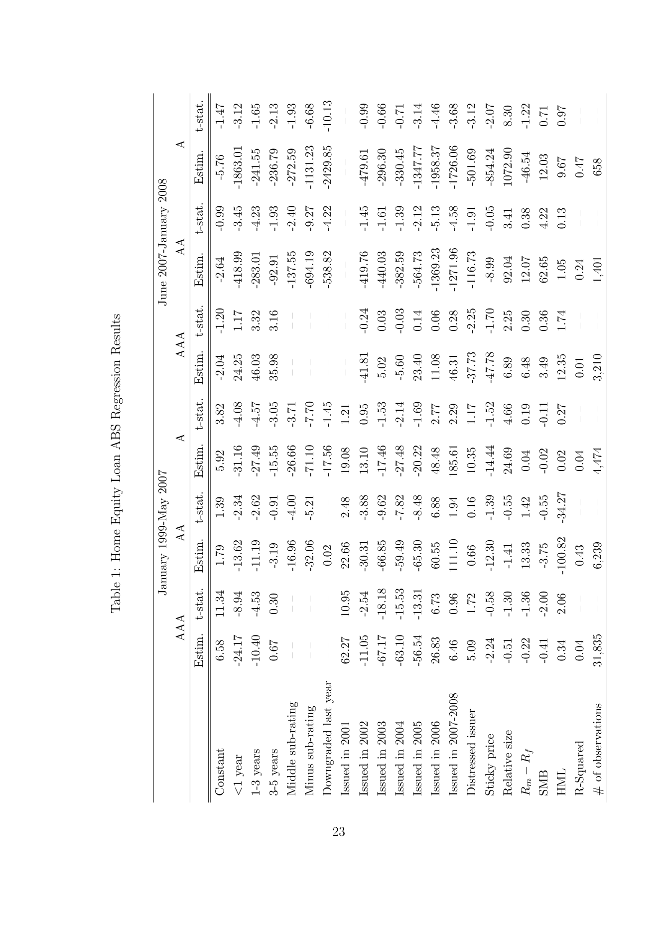
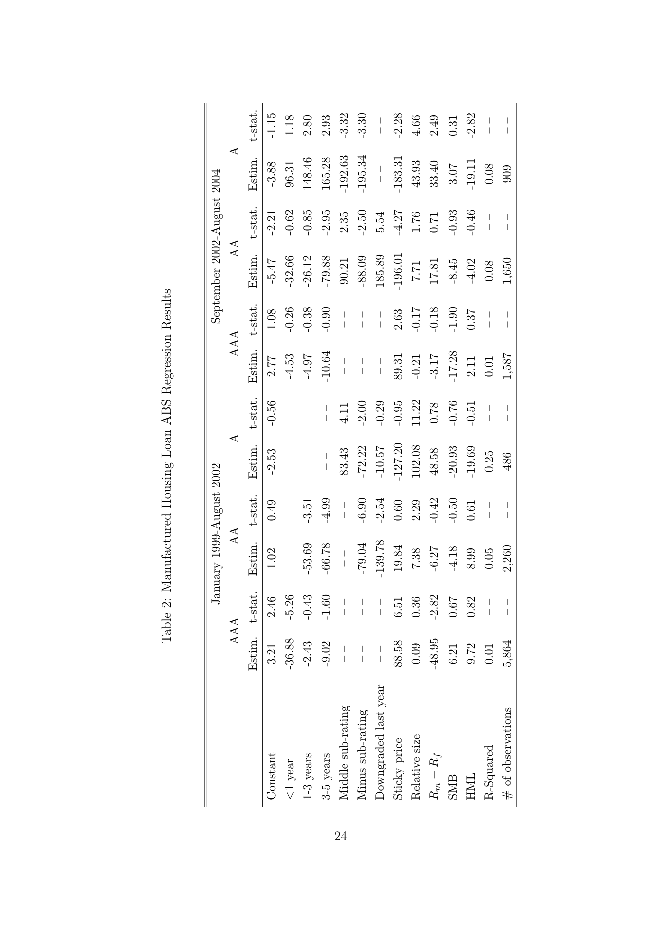
To distinguish between these possible explanations, we regress the fit errors on a set of explanatory variables for crisis and pre-crisis periods. The results are reported in Tables 1 and 2.

In our regressions, we pool the data for different dates but allow for autocorrelation in the residuals for individual securities and for temporal heteroskedasticity.

Specifically, we run a preliminary regression, estimate autocorrelations for each security’s residuals, average the estimated correlation coefficients and perform a Prais- Winsten transformation before repeating the regression. As a last stage, we calculate the volatility of the residuals in the second stage regressions for each time period and then perform a final regression with weighted least squares. Details of the econometric implementation are provided in an appendix.

Many of the regressors we employ are dummy variables. The omitted category is a tranche that (i) has greater than a 5-year maturity, (ii) has a high sub-rating (i.e., is AA+ or A+ if it is not AAA), (iii) was not downgraded in the last year, (iv) was issued prior to 2001 (in the case of HEL) (v) does not have an issuer in financial distress (in the case of HEL).

Recall that we employ two liquidity variables: (i) ‘sticky price’ (the fraction of observations in the last month for which the bid price did not change), and (ii) relative size (the share of the issue volume in the total volume of issues included in the index measured in basis points).

Coefficients of relative size variable are not of consistent sign for either HEL or MH. We do observe substantial impacts and statistic significance for HEL during crisis time but the effects are not present for MH exposures in the corresponding crisis period for that exposure class. This result is to be expected since the MH crisis was not accompanied by a big increase in the market premium on liquidity.

In the case of HEL regression, sticky price variable exhibits the correct sign throughout the sample period and the coefficient is significant in most cases. In the case of the MH regressions, however, we observe inconsistent coefficient signs and a lack of significance.

The risk premium variables are betas obtained from prior regressions of log price changes on Fama-French factors. Most of the coefficients are negative as one might expect but the statistical significance is not great.

On differences between the market and the ratings agencies’ assessments of credit quality, the strong and intuitively reasonable effects of the sub-ratings variables and their statistical significance suggest consistency.

However, a highly significant and economically important variable is the dummy for a down-grade within the last year. In the crisis period regressions, this becomes extremely large. This is evidence of a strong momentum effect: the market expects issues that have been downgraded to be further down-graded in the future and allows for this in its pricing of the issue.

The corresponding parameter in the MH ABS regression is positive in the crisis period. When a security is down-graded, if the market agrees with the rating agency evaluation, one might expect the parameter to be positive as the security would be viewed as relatively high quality within the new lower rating category.

We found that the market appears to favor distressed issuers in non-crisis time but punishes them substantially during crises. This could be explained by the fact that the ‘distressed issuers’ are among the largest 14 issuers and hence their issues may enjoy a liquidity premium in non-crisis periods. But when a crisis has affected a sector their issues will be substantially discounted.

For the HE regressions, the ’issue year’ dummies suggest the vintage is extremely important in the crisis periods, suggesting the market perceived a marked deterioration in pool quality.

As a second exercise, for the HEL securities, we perform a sequence of purely crosssectional regressions month by month (i.e., not pooling across the data for different months) starting in June 2007. The results are shown in Figures 5, 6 and 7.

Figure 5 shows the regression coefficients for the sticky price variable, month by month in the crisis period. The coefficients for AA and A (see Panels B and C) follow time paths that are qualitatively similar with substantially negative values appearing in the autumn of 2007.

A striking observation is the degree to which the AA and A parameters are negatively correlated with the spread between USD Libor and US Treasuries which is shown in Panel D of Figure 5. This spread, which has reached unprecedented levels over the last year is an indicator of the crisis of confidence in their counter-parties that the banks have experienced over the last year. It is very striking that the time path of this variable is so clearly negatively correlated with an indicator of the illiquidity premium, our sticky price coefficients.

Figure 6 shows the path over time of the coefficients on the risk-factor beta regressors. The magnitudes and even sign of the risk factor effects vary over time and there is no very clear pattern that emerges.

Figure 7 shows the time paths of coefficients on dummy variables for the year of the issue. Especially for the AA and A grade results, there is a very clear pattern with discounts being larger for later issue years. In the case of the A grades, the discounts grow monotonically as time goes by, achieving discounts of more than 30 by early 2008 in the case of deals issued in 2006 and 2007.

The size of these issuance-year-dummy coefficients indicates the extreme aversion to investing in recently issued deals that many market participants have. One could the results shown in Figure 7 as reflecting disagreement between the market and ratings agencies about the credit quality of the issues in question. Or it is possible that investors require a large risk premium to compensate them for a risk associated with issues such as the risk that underwriting standards will prove to have been particularly low after a certain date.

5 Conclusion

In credit crises, market pricing can exhibit unusually large variation. This variation can provide an interesting ‘laboratory’ for understanding the pricing of securities in general.

In this paper, we investigate the major variation in the pricing of individual ABS tranche issues in two periods of market stress: (i) the collapse in the Manufactured Housing ABS sector in 2002 and (ii) the turmoil in the Home Equity Loan ABS sector in 2007.

We find that conventionally defined risk premia contribute relatively little to the cross-sectional variation of ABS. Liquidity as proxied by a simple measure of price stickiness contributes a sizeable share of discounts cross-sectionally. In the crisis and 2007-2008, regression coefficients for this liquidity proxy move over time in a way that closely reflects changes in the spread between USD Libor and US Treasury yields, an indicator of banks’ concerns about their counter-party risk and liquidity.

Even allowing for liquidity, risk premia and the rating, ABS prices in the 2007- 2008 crisis are highly sensitive to the year of issue of HEL ABS securities. This could either reflect disagreement between the market and the ratings agencies evaluations of deals or it might reflect a substantial risk premium associated with uncertainty about the degree of deterioration in under-writing in the home equity loans that back these deals.

References

A., K., D. Yang, and F. J. Fabozzi (2004): “An Option-Theoretic Prepayment Model for Mortgages and Mortgage-Backed Securities,” International Journal of Theoretical and Applied Finance, 7(8).

Altman, E. I. (2007): “Global Debt Markets in 2007: New Paradigm or the Great Credit Bubble?,” Journal of Applied Corporate Finance, 19(3), 17–31.

Bliss, R. R. (1997): “Testing Term Structure Estimation Methods,” Advances in Futures and Options Research, 9, 197–231.

Chen, L., D. Lesmond, and J. Wei (2007): “Corporate Yield Spreads and Bond Liquidity,” Journal of Finance, 62.

Chomsisengphet, S., and A. Pennington-Cross (2006): “The Evolution of the Subprime Mortgage Market,” Federal Reserve Bank of St. Louis Review, 88, 31–56.

Davidson, A. (2003): Mortgage-Backed Securities Prepayments, Securitization: Structuring and Investment Analysis. Wiley.

de Jong, F., and J. Driessen (2006): “Liquidity Risk Premia in Corporate Bond Markets,” mimeo, University of Amsterdam, Amsterdam.

Demyanyk, Y., and O. Van Hemert (2007): “Understanding the Subprime Mortgage Crisis,” Working paper, New York University.

Downing, C., R. Stanton, and N. Wallace (2005): “An Empirical Test of a Two-Factor Mortgage Valuation Model: How Much Do House Prices Matter?,” Real Estate Economics, 33, 681–710.

Elton, E. J., M. J. Gruber, D. Agrawal, and C. Mann (2001): “Explaining the Rate Spread on Corporate Bonds,” Journal of Finance, 56(1), 247–277.

Ericsson, J., and O. Renault (2006): “Liquidity and Credit Risk,” Journal of Finance, 61(5), 2219–2259.

Fender, I., and P. Hordahl (2007): “Overview: credit retrenchment triggers liquidity squeeze,” BIS Quarterly Review, pp. 1–16.

Ferguson, R., and S. Raymar (1998): “A Comparative Analysis of Several Popular Term Structure Estimation Models,” Journal of Fixed Income, 8, 17–33.

Harfush-Pardo, M., W. Perraudin, and S. Wu (2008): “Credit Term Structure Fits with Risk Adjusted Transition Matrices,” Working paper, Risk Control Limited, London.

Houweiling, P., J. Hoek, and F. Kleibergen (2001): “The joint estimation of term structures and credit spreads,” The Journal of Empirical Finance, 8, 297–323.

Huang, W., and J. Ondrich (2002): “Stay, Pay, or Walk Away: A Hazard Rate Analysis of Federal Housing Administration-Insured Multifamily Mortgage Terminations,,” Journal of Housing Research, 13(1).

Jarrow, R. A., D. Lando, and S. M. Turnbull (1997): “A Markov Model for the Term Structure of Credit Spreads,” Review of Financial Studies, 10, 481–523.

Kau, J. B., and D. C. Keenan (1995): “An Overview of the Option-Theoretic Pricing of Mortgages,” Journal of Housing Research, 6(2).

Keys, B., T. Mukherjee, A. Seru, and V. Vig (2008): “Securitization and Screening: Evidence From Subprime Mortgage Backed Securities,” Working paper.

Kijima, M., and K. Komoribayashi (1998): “A Markov Chain Model for Valuing Credit Risk Derivatives,” Journal of Derivatives, 5(Fall), 97–108.

Lamb, R., M. Harfush-Pardo, and W. Perraudin (2007): “Ratings-Based Pricing and Stochastic Spreads,” Working paper, Imperial College, London.

Large, A. (2005): “Financial Stability: Managing Liquidity Risk in a Global System(,” Financial Stability Review, pp. 78–84.

Longstaff, F., S. Mithal, and E. Neis (2005): “Corporate Yield Spreads: Default Risk or Liquidity? New Evidence from the Credit Default Swap Market,” Journal of Finance, 60(5), 2213–2253.

McCulloch, J. (1975): “The Tax-Adjusted Yield Curves,” Journal of Finance, 30(3), 811–30.

McCulloch, J. H. (1971): “Measuring the term structure of interest rates,” Journal of Business, 44, 19–31.

Mian, A., and A. Sufi (2008): “The Consequences of Mortgage Credit Expansion: Evidence from the 2007 Mortgage Default Crisis,” Discussion paper, University of Chicago mimeo.

Morgenson, G. (2007): “Inside the Countrywide Financial Lending Spree,” New York Times.

Nelson, C. R., and A. F. Siegel (1987): “Parsimonious Modeling of Yield Curves,” The Journal of Business, 60, 473–489.

Perraudin, W., and A. Taylor (2007): “Liquidity, Bond Market Spreads and Conditional Risk Premia,” mimeo, Imperial College, London.

Schwartz, T. (1998): “Estimating the term structure of corporate debt,” Review of derivatives research, 2, 193–230.

Shea, G. (1984): “Pitfalls in Smoothing Interest Rate Term Structure Data: Equilibrium Models and Spline Approximations,” Journal of Financial and Quantitative Analysis, 19, 253–269.

Spahr, R. W., and M. A. Sunderman (1992): “The Effect of Prepayment Modeling in Pricing Mortgaga-Backed Securities,” Journal of Housing Research, 3(2).

Turnbull, S. M. (2008): “The Credit Crisis of 07,” mimeo, University of Houston, Houston, Texas.

Vasicek, O., and H. Fong (1982): “Term Structure Modeling Using Exponential Splines,” Journal of Finance, 37(2), 339–356.

Appendix

A Spread Term Structure Fits

This appendix provides more detail on the transition-matrix approach to fitting defaultable debt spread term structures for different ratings categories.

Consider a set of bonds with ratings from the set {1, 2, ..., J} and prices Bi i = 1, 2, ..., N. Ji X (A1) Bi = ci,j exp[−(rτi,j + Sτ(i,jr) )τi,j] j=1 where ci,j for j = 1, 2, ..., Ji are the cash flows of bond i and the τi,j are the cash flows dates for j = 1, 2, ..., Ji. Suppose that the τ dates are discretized so that the τi,j are all integers and that ratings evolve accordingly to a Markov chain with transition matrix[2] M. The transition matrix has the following shape:

. . . θ1,1 θ1,2 θ1,R θ1,D . . . θ2,1 θ2,2 θ2,R θ2,D M = ... ... ... ... ... (A2)

0 0 . . . 0 1

where θi,j denotes the probability of a bond moving from rating i to rating j in one year, for j, i = {1, 2, ..., R}. The last column and row of the transition matrix M represent the probability of defaulting and it is denoted by θi,D for i = {1, 2, ..., R}. The default probabilities at horizons 1, 2, ..., 30 years are the right hand column of powers of M. Let θi,D(j) be the right hand column of the jth power of M, for j = {1, 2, ..., 30} and for i = {1, 2, ...R}. The survival probability of a bond at time j conditional on rating i at time zero, denoted by Pi(j), is defined as follows: Pi(j) = 1 − θi,D(j) (A3)

Given a time homogenous transition matrix M, we can price a bond i as,

Ji X (1 − γ)] (A4) B˜i = ci,j exp[−rjj][γ + Pi(j) j=1 where γ is the expected recovery rate and it is constant across all rating categories; and rj is Treasury zero-coupon interest rate for a bond with maturity j. If M is parameterized in a suitable manner, M = M(θ˜), we can minimized the sum of the squared differences between the model and the observed prices over the vector θ˜. To enforced appropriate properties for M(θ˜), we parameterize it as

0 . . . 1 − Φ(θ˜[1],[2]) − Φˆ[1] Φ(θ˜[1],[2]) ˆΦ[1] . . . Φ(θ˜[2],[1]) 1 − Φ(θ˜[2],[1]) − Φ(θ˜[2],[3]) − Φˆ[2] Φ(θ˜[2],[3]) ˆΦ[2] M(θ˜) = (A5) ... ... ... ... ...

0 0 0 0 1

where,

ˆΦ[1] Φ(θ˜[1],D) ˆΦ[2] Φ(θ˜[1],D) + Φ(θ˜[2],D) = . (A6) ... ...

PR ˆΦR i=1 Φ(˜θi,D) Here, Φ(.) represents the cumulative standard normal distribution. We present the algorithm to estimate the parameters θ˜ in the next section. The constraints for the problem is that the elements on the diagonal are less or equal to 1.

This approach to fitting term structures may be thought of as one of parameterizing a ratings-based credit derivative pricing model such as those of Jarrow, Lando, and Turnbull (1997), Kijima and Komoribayashi (1998) and Lamb, Harfush-Pardo, and Perraudin (2007). These models assume that time-varying (rather than timehomogeneous, as in our case) ratings transition matrices are fitted to market price data and then the inferred risk-adjusted processes may be used to price more complex credit derivative contracts. In the context of this paper, we prefer to think of our approach as an interpolation technique for ordered credit spreads rather than as an implementation of a theoretical model.

B Pre-Payment Assumptions

Due to the complexity and importance of prepayment measure, we here describe the prepayment measure data we employ. For any given ABS tranche, Bloomberg reports one of 7 different prepayment measures:

1. CPR (Constant Prepayment Rate), also know as conditional prepayment rate, measures prepayments as a percentage of the current outstanding loan balance. It is always expressed as a compound annual rate. It is commonly used to describe the prepayment experience of Home Equity Loans and student-loan assets.

Definition from Bloomberg: Constant Prepayment Rate (CPR). Annualized equivalents of single monthly mortality (SMM). CPR attempts to predict the percentage of principal that will prepay over the next 12 months based on historical principal pay-downs. CPR is measured on 1 month, 3 month, 6 month, 12 month, or since issue basis. CPR = 100∗(1−(1−SMM/100)(12/monthsinperiod)).

2. HEP (Home-Equity Prepayment Curve). CPR will get to that level in 10 months and stay stable afterwards.

Definition from Bloomberg: The ”HEP” (Home Equity Prepayment) curve is a prepayment measurement scale with a 10-month seasoning ramp, as compared to the 30-month ramp for the PSA curve. The HEP scale ranges from 0% to 100%. A HEP value corresponds to the terminal 10th month CPR speed – having evenly stepped the preceding 9 months. For example, 20% HEP corresponds to 2% the 1st month, 4% the 2nd, and 20% the 10th month and thereafter. (The HEP scale was developed by Prudential Securities, and it reflects their extensive research of home equity prepayment experience.)

3. PPC (Prospectus Prepayment Curve). Sometimes called the pricing prepayment curve, the PPC is a relatively new convention, used mainly with HELs and is always issue-specific. However in our calculation we uniform all PPC measure by using 100% PPC equals CPR from 10.8% to 27.5% in 30 months and stay stable afterwards.

Definition from Bloomberg: “PPC” is Bloomberg’s prepayment rate notation corresponding to “Prospectus Prepayment Curve” or “Pricing Prepayment Curve”. For example ”100 PPC” and ” 150 PPC” correspond to prepayment scenarios of 100% and 150% of a prepayment curve as defined in the prospectus for an indicated bond. Bonds with “PPC” cash-flows are usually priced at 100% PPC, though not necessarily so. Bonds with “PPC” cash-flows may also have other cash-flows for other prepayment rates such as CPR, PSA, etc. When available,

PPC rates can be used in all Bloomberg analytics by replacing an alternative prepayment specification. As a time-saver, function YPPC automatically utilizes up to seven PPC scenarios in the familiar YT function format.

4. MHP (Manufactured-Housing Prepayment Curve. 100% MHP equals CPR from 3.7% to 6% in 24 months and stay stable afterwards.

Definition from Bloomberg: The “MHP” (Manufactured Housing Prepayment) curve is a prepayment scale with a 24-month seasoning ramp. A prepayment rate of 100% MHP equates to a starting rate of 3.7% CPR, which then evenly steps .1% per month and terminates at 6% on the 24th month. 200% MHP would then start at 7.4%, step by .2%, and terminate at 12%. The MHP Curve was developed by Lehman Brothers as a result of their prepayment research efforts.

5. PSA (Public Security Association Prepayment Model). Standard 100% PSA equals CPR from 0 to 6% in 30 months and stay stable afterwards.

Definition from Bloomberg: Prepayment Standard Assumption (PSA). The PSA is a percentage expression of the relationship between the actual and expected CPR based on the PSA prepayment assumption ramp. The ramp assumes mortgages prepay slower during their first 30 months of seasoning. 100% PSA indicates a starting rate of .2% CPR increasing .2% per month for the first 30 months. A constant 6% CPR is assumed for the remaining life of the mortgage. To calculate PSA, use the following formula: PSA = [CPR/(.2)(m)] * 100, where m = number of months since origination of the underlying loans

6. MPR (Monthly Payment Rate) Technically this is not a prepayment measure, because it is used with non-amortizing assets, such as credit card and dealer floor-plan receivables, which are not subject to prepayment. Rather, the MPR is a repayment measure and is calculated by dividing the sum of the interest and principal payments received in a month by the outstanding balance.

7. Absolute Prepayment Speed (ABS) Definition from Bloomberg: Absolute Prepayment Rate (ABS) is the standard measure of prepayments for automobile loan backed securities. ABS calculates prepayments as the percent of original dollar balance of receivables.

Among the Home Equity Loan tranches prepayment type 1, 2 and 3 are widely and generally equally quoted. There are a small number of them are quoted in type 5.

Of these measures, for Home Equity Loan ABS, Bloomberg supplies one of three prepayment measures: CPR, HEP and PPC. For Manufactured Housing ABS, Bloomberg supplies just the MHP measure. In our calculations, we transform all the different measures into CPR and then use them in our cash flow estimation.

C Panel Data Structure and Autocorrelation

We perform an Ordinary Least Squares regression of the fit errors on our explanatory variables. One may expect that the residuals from this regression corresponding to a particular security are autocorrelated over time. We assume that the regression equation takes the form:

(C1) yi,t = β′xi,t + ei,t (C2) ei,t = ρei,t−1 + νi,t

for time periods t and securities i. Here, y are the fit errors, x is a vector of explanatory variables and the νt are serially uncorrelated, homoskedastic errors, independent across i with variance σν[2] and dependent on time t. To adjust for the autocorrelation, we use a Prais-Winsten transformation. Details are as follows.

1. We run an ordinary least squares regression of the fit errors y, pooled across time and securities, on the explanatory variables, x. We calculate the fitted residual vector, eˆ;

2. For each security, we calculate the correlation coefficient, ρi, between ei,t and ei,t−1;

3. We average the estimated individual-exposure correlation coefficients, ρˆi to obtain a mean, fitted correlation coefficient ρˆ;

4. We calculate transformed data: p p y[1]∗ ≡ 1 − ρˆ[2]y[1] x∗[1] ≡ 1 − ρˆ[2]x[1] (C3) p p yt∗ ≡ 1 − ρˆ[2]yt−[1] x∗t ≡ 1 − ρˆ[2]xt−[1] (C4)

5. Perform a regression of y∗ on x∗.

Table 1Copy link

Table 2Copy link

Notes

∗We thank Mariam Harfush-Pardo and Diep Ho. The authors’ may be contacted at Tanaka Business School, Imperial College, London SW7 2AZ or at s.wu06@imperial.ac.uk or wper- raudin@imperial.ac.uk. 1Source: Merrill Lynch Global Index Rules 2007. 2The transition matrix is assumed to be in annual terms.