

This paper develops a simple but rigorous approach to allowing for default probability risk in securitisation capital calculations. The approach consists of including additional random factors to describe risk in inputs, specifically default probabilities for pool loans. We show that the addition of such “parameter risk” translates into more conservative correlation assumptions for the asset correlations of the underlying loans. Parameter risk is, hence, relevant for banks’ on-balance-sheet loans just as much as for securitisations secured on those loans. To the extent that parameter risk is correlated with systematic risk driving the bank’s wider portfolio, capital for loans should be increased. Securitisation capital, which depends on pool capital, should, in turn, be higher as well. Parameter risk does not justify boosting securitisation capital for all the tranches in a deal beyond the level implied by prudent calculation of pool capital. It, therefore, does not provide an argument for deviations from capital neutrality under which the capital for all the tranches in a securitisation should equal that for the securitisation loan pool. (Reasons for non-neutrality includes the presence of agency costs created in complex, multi-agent securitisation processes.) We believe that the Basel Committee allowed for parameter input risk in its original calibration of the Basel II capital risk weights for on-balance-sheet loans. Those involved in the calibration of Basel II were clearly aware that the correlation parameters employed in the Basel II risk weight functions were higher than those implied by statistical analysis of bank loan default data. Our analysis shows that except where parameter risk implies higher pool capital, the impact on securitisation capital is relatively small. In particular, if parameter risk is correlated with intra-pool risk factors but is not systemic, then it justifies some limited shifting of capital towards more senior tranches. One might note that, if this latter type of parameter risk is present, the case for deduction of thin tranches attaching just below pool capital (a misguided and unjustified feature of current and proposed regulations) is even weaker.
Summary
This paper develops a simple but rigorous approach to allowing for default probability risk in securitisation capital calculations. The approach consists of including additional random factors to describe risk in inputs, specifically default probabilities for pool loans. We show that the addition of such “parameter risk” translates into more conservative correlation assumptions for the asset correlations of the underlying loans.
Parameter risk is, hence, relevant for banks’ on-balance-sheet loans just as much as for securitisations secured on those loans. To the extent that parameter risk is correlated with systematic risk driving the bank’s wider portfolio, capital for loans should be increased. Securitisation capital, which depends on pool capital, should, in turn, be higher as well.
Parameter risk does not justify boosting securitisation capital for all the tranches in a deal beyond the level implied by prudent calculation of pool capital. It, therefore, does not provide an argument for deviations from capital neutrality under which the capital for all the tranches in a securitisation should equal that for the securitisation loan pool. (Reasons for non-neutrality includes the presence of agency costs created in complex, multi-agent securitisation processes.)
We believe that the Basel Committee allowed for parameter input risk in its original calibration of the Basel II capital risk weights for on-balance-sheet loans. Those involved in the calibration of Basel II were clearly aware that the correlation parameters employed in the Basel II risk weight functions were higher than those implied by statistical analysis of bank loan default data.
Our analysis shows that except where parameter risk implies higher pool capital, the impact on securitisation capital is relatively small. In particular, if parameter risk is correlated with intra-pool risk factors but is not systemic, then it justifies some limited shifting of capital towards more senior tranches. One might note that, if this latter type of parameter risk is present, the case for deduction of thin tranches attaching just below pool capital (a misguided and unjustified feature of current and proposed regulations) is even weaker.
Introduction
This note explains how one may allow for uncertainty about pool default probabilities in setting capital for securitisation tranches.[1] We develop a direct and rather natural way of introducing default probability uncertainty by including additional factor risk into the capital calculation.
The issue of default probability uncertainty in securitisation capital has been recently raised by Antoniades and Tarashev (2014). These authors suggest adding to capital the expected value of any positive undercapitalisation. To illustrate, they calculate such undercapitalisation for securitisation tranches within the framework of an asymptotic single risk factor (ARSF) model.
1 This note was prepared by William Perraudin, Director, Risk Control.
Capital for securitisation tranches derived using an ASRF model is effectively degenerate in that it jumps from full deduction to zero at the attachment point corresponding to pool capital. In this case expected positive undercapitalisation will peak at roughly a half almost by construction. Using their particular distribution for pool capital, Antoniades and Tarashev obtain an under-capitalisation of 60%.
Their result is not at all robust, however, in that when Antoniades and Tarashev employ capital models in which the thin tranche capital is smoother and less of a step function, expected positive undercapitalisation is much lower. For example, when they use a two factor model like that employed by the Basel Committee in its latest BCBS (2013) discussion paper on securitisation capital, the capital adjustment drops from 60% to 6%.
Perraudin (2015) comments on Antoniades and Tarashev (2014) developing arguments similar to those above. It also argues that these authors’ focus on securitisation tranches that attach in the vicinity of pool capital which they refer to as “mezzanine ranches” is scarcely relevant for actual mezzanine tranches in Europe which commonly attach at multiples of between 2 and 3 times pool capital.
In addition to the above points, however, one may take issue with the expected, positive under-capitalisation approach to default probability risk advocated by Antoniades and Tarashev. There is a much more obvious and direct way of analysing default probability risk in securitisation capital than that which they employ.
The direct approach consists of calculating capital explicitly allowing for default probability uncertainty. In effect, this uncertainty boosts factor risk in the capital calculation. The effects depend both qualitatively and quantitatively on how this additional factor risk is correlated with other sources of factor risk affecting the performance of the securitisation pool.
This note sets out this alternative approach, in some detail, within the framework of the two factor model of securitisation capital. The two factor model was originally proposed by Pykhtin and Dev (2002). It was extended to allow for imperfect granularity and multiple time periods by Duponcheele et al (2013b) and (2013c). Calibration of a simplified, conservative version of the two factor model was provided by Duponcheele et al (2014a).[2]
We believe that the approach we propose in this note helps to reveal the true implications of default probability risk for securitisation capital. In particular, we argue that the Basel Committee’s calibration of capital for onbalance-sheet loans already allows for default probability risk. We document this by references to research studies published by regulators involved in the Basel II calibration early on in the process of that calibration.
We show that if pool capital is already conservatively adjusted for estimation risk, then the case for significant further adjustments of securitisation capital is relatively weak and must rely on the assumption that the estimation risk is correlated with non-systematic, intra-pool correlation. To the extent that such correlation is a concern, it may be tackled by using somewhat conservative values for intra-pool correlations which is the approach that we ourselves have taken in our past calibration studies (see, most notably, Duponcheele et al (2014a)).
1. Thin Tranche Capital in a Two Factor Model
We begin, in this section, by developing the assumptions of the two-risk-factor model used by the Basel authorities in calibrating the current BCBS 303 proposals. In this model, the asset values of individual obligors are presumed to be driven by Gaussian random variables. An obligor defaults, over a one year period, if its asset value falls below a certain threshold or “trigger” level. Formally, a given obligor defaults if an associated random variable Z satisfies: Z< c where Z~N(0,1) (1)
Prob(default) = Φ(c) ≡p (2)
We suppose that Z depends linearly on common factors, f and g, and an idiosyncratic shock ε.
(3)

2Duponcheele et al (2014b) and (2014c) then used this to calibrate variants of the reduced form Simplified Supervisory Formula Approach (SSFA) proposed by the Basel regulators (in BCBS (2014)) as a basis for securitisation regulatory capital.
Here, the three random variables are mutually uncorrelated and f, g, ε ~N(0,1).
We shall assume, in what follows, that the risk factor f represents the single source of randomness driving defaults in the diversified portfolio of the bank for which we are analysing capital. One may then calculate the marginal Value at Risk (with a confidence level 1 −α) of a loan held by the bank as the Expected Loss on that loan conditional on f equalling its α-quantile. We assume that the fractional recovery on the loan is independent of f and has a mean equal to LGD. In this case, the marginal VaR for the loan will equal
(4) MVaR_{Loan} = Prob(default|f= f_α) × LGD
Under the above assumptions, it is straightforward to calculate the probability of default of an individual loan conditional on f= f_α:

Under the usual Basel II assumptions α= 0.1%, the per dollar of par capital for a loan is:
(6)

Here, K_{IRB} = p_α × LGD is the marginal VaR per dollar of par value for a one-year maturity loan.[3]
So far, we have focussed on individual loans. Now, we turn to losses on diversified portfolios of loans. Vasicek
(2002) shows that the distribution (denoted W(θ)) of the fraction of a diversified pool of loans that defaults (denoted θ)is:

where (8)

In what follows, we suppose that the par value of the pool is normalised to unity (without loss of generality). Hence, W(θ) is the distribution of pool defaults.
Assume that the loss given default of pool loans is constant (and denoted LGD). The expected loss of a thin securitisation tranche (with attachment point A) secured against this pool is:

One may calculate the marginal VaR for the thin tranche position held within the bank’s wider diversified portfolio, as the expected loss conditional on f= f_α. For a thin tranche attaching at A, this implies a marginal VaR equal to:

where (11)

Note that the marginal VaR depends on the conditional probability of default of individual loans, p_α, and on the conditional correlation of risk factors for any two individual pool loans, ρ_{pool,α}.
Hence, the above result may be written as:
3 In practice, there are some additional complexities here in that, in the Basel Internal Ratings Based Approach (IRB), regulatory capital is based on Unexpected Loss K multiplied by 1.06. Thus, one may use the notation: KIRBA=K×1.06. European regulation defines KIRB=K×1.06+EL1==KIRBA+EL[1], where EL[1] is the one-year expect loss. There is some disagreement as to the rationale for the 1.06 scaling factor. Some say it was introduced in order to align Basel II capital on average with Basel I capital levels upon the introduction of the former. However, others suggest it is an adjustment for model risk.

If the capital for a thin tranche is based on the above marginal VaR formula, one may be concerned about risk associated with mis-measurement in the underlying inputs. Antoniades and Tarashev focus on risk associated with mis-measurement of p which will be inherited by p_αand K_{IRB}which depend on p. In the next section, we develop a simple way of adjusting for such mis-measurement in capital calculations.
2. Thin Tranche Capital with Default Probability Risk
Suppose that the trigger level for default, c, is observed with error, in that a given loan defaults if:
_2) (13) Z< c−v v~N(0, σ[_v]
Introducing randomness in the trigger level c is equivalent to supposing that the default probability is known with error. As we shall see, the effects on capital of the uncertainty depend on how v is correlated with other sources of risk.
Suppose that: (14)
](/api/media/file/eq-51-300x17.png?prefix=media)
(15) e~N(0,1) and cov(e, g) = cov(e, f) = 0
This allows for the fact that the model uncertainty might be systematic in that it is correlated with the factor, f, that drives the bank’s wider portfolio. Alternatively, it might be correlated with the additional factor risk present in the securitisation pool, g. Lastly, it might serve to introduce a third common factor, e.
If equations (14) and (15) apply, default occurs if:
![Equation: ρf+ 1 −ρ ρ∗g+ 1 −ρ 1 −ρ∗ε+ σ[_v] λ_ff+ σ[_v] λ_gg+ σ[_v] 1 −λ_f −λ_ge< c (15)](/api/media/file/eq-52-300x11.png?prefix=media)
One may again derive the default probability of an individual loan and the correlation of latent variables driving any two loans both unconditionally and conditional on the systematic factor, f, that drives the bank’s wider portfolio. In so doing, one obtains:


Here:
![Equation: ∆= ( ρ+ σ[_v] λ_f)_2 + ( 1 −ρ ρ∗ + σ[_v] λ_g)_2 + σ[_v]_2 1 −λ_f −λ_g + (1 −ρ)(1 −ρ∗) (18)](/api/media/file/eq-55-300x12.png?prefix=media)
![Equation: ∆_α= ( 1 −ρ ρ∗ + σ[_v] λ_g)_2 + σ[_v]_2 1 −λ_f −λ_g + (1 −ρ)(1 −ρ∗) (19)](/api/media/file/eq-56-300x14.png?prefix=media)
And:

(20)

(21)

To obtain thin tranche capital inclusive of the effects of default probability risk one may simply plug these

3. Special Cases
In this section, we examine some special cases. These correspond to situations in which the default probability risk is (i) perfectly correlated with the systematic factor driving the bank portfolio, f, (ii) perfectly correlated with the additional pool factor, g, or (iii) orthogonal to both f and g but still common to all individual loans. The third case, in effect, introduces a third factor, e.
When λ_g = 0 ; λ_f = 1

(23)

In this case, which one might guess would represent the most conservative assumption for capital, the conditional loan default probability is increased but the intra-pool correlation parameter is unchanged.
Suppose, instead that λ_f = 0 ; λ_g = 1. In this case:


increased by introducing default probability risk.
When λ_f = λ_g = 0


expressions into equation (10), one obtains the marginal VaR or capital level for a thin tranche attaching at A.
4. Calculations
In this section, we present illustrative calculations of capital inclusive of default probability risk. We employ the parameters for European Small and Medium Enterprise (SME) loan backed securitisations proposed by Duponcheele et al (2014a). These parameters, summarised in Table 1, reflected the views of a group of securitisation risk experts from major banks, the AFA Quant Group.
We set p_0 equal to the default probability, 0.94%, and infer the original threshold level of default as c_0 = Φ_{−1}(p_0, 0,1). We can infer the distribution of default probability p using the relation: p= Φ(c_0 −v, 0,1) and the

fact that v is normal with a volatility of σ[_v], (i.e., v~N(0, σ[_v]
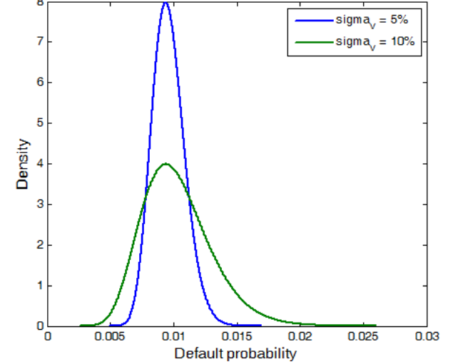
Figure 1 shows the density of default probabilities given the randomness in v and the assumed values for σ[_v] of 5% and 10%. As one may observe, instead of taking its true value of 0.94%, the default probability ranges from around 0.75% to 1.17% when σ[_v] = 5% and from around 0.6% to 1.45% when σ[_v] = 10%.[4]
4 The ranges are calculated based on 5% and 95% confidence levels.
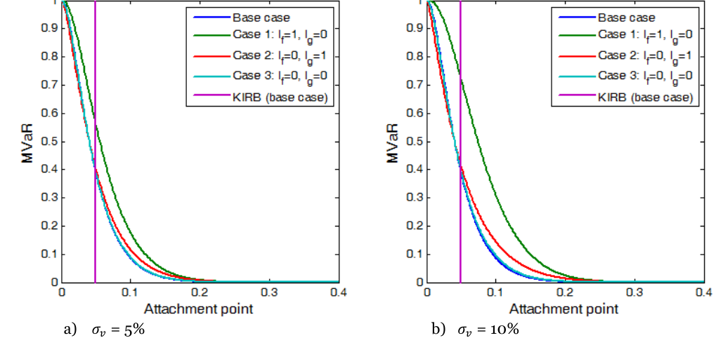
We calculate thin-tranche capital in the base case and in the three special cases described above and plot the results, for the two values of σ[_v] we consider in Figure 2. (The assumptions for the input parameters are given in Table 1.)
From Figure 2, one may observe that thin tranche capital in special case 3 is very close to the base case. Thin tranche capital in Case 2 is higher than the base case for attachment points above K_{IRB} (which here equals 4.9%) and is slightly lower for attachment points lower than K_{IRB}. The magnitude of the boost to capital in Case 2 is clearly larger when σ[_v] takes the higher of the two values we consider.
Special case 1 exhibits the largest impact on capital when default probability risk is introduced. When σ[_v] = 10%, the whole capital curve shifts to the right.
Table 2 shows the impact of the different scenarios (under different assumptions about the value of σ[_v]) on the inputs to the capital calculations, i.e., the conditional default probabilities, the conditional correlations between

How should one interpret the results so far presented? Introducing default probability risk justifies an increase in pool capital. This is then translated into higher capital for securitisation tranches. Such risk boosts K_{IRB} which feeds through into a rightward shift of the thin tranche capital curve at least in the most extreme case in which the default probability risk is highly correlated with the risk factor, f, that drives the bank’s wider portfolio.

a) σ[_v] = 5% b) σ[_v] = 10%
Does this constitute an argument for higher capital for securitisation tranches? The answer is: only in so far as one has not already been conservative about the capital input, K_{IRB}. And, indeed, the default probability risk is, in this sense, just as important for on balance sheet capital calculations as for securitisation capital. In both cases, it justifies a conservative approach.

actual levels of these parameters employed and the factor weights are shown in Table 3.

| ρpool,α | ||||||
|---|---|---|---|---|---|---|
| Case | pα | KIRB | λf λg | |||
| Base | case | 0.11 | 0.15 | 0.05 | ||
| σv = | 5% | |||||
| Case | 1 | 0.14 | 0.15 | 0.06 | 1 | 0 |
| Case | 2 | 0.11 | 0.19 | 0.05 | 0 | 1 |
| Case | 3 | 0.11 | 0.15 | 0.05 | 0 | 0 |
| σv = | 10% | |||||
| Case | 1 | 0.19 | 0.15 | 0.08 | 1 | 0 |
| Case | 2 | 0.12 | 0.23 | 0.05 | 0 | 1 |
| Case | 3 | 0.11 | 0.16 | 0.05 | 0 | 0 |
| ρpool,α | |||||
|---|---|---|---|---|---|
| Case | pα | λf λg | |||
| Base | case | 0.11 | 0.15 | ||
| σv = 5% | |||||
| Case | 1 | 0.11 | 0.15 | 1 | 0 |
| Case | 2 | 0.11 | 0.19 | 0 | 1 |
| Case | 3 | 0.11 | 0.15 | 0 | 0 |
| σv | = 10% | ||||
| Case | 1 | 0.11 | 0.15 | 1 | 0 |
| Case | 2 | 0.11 | 0.23 | 0 | 1 |
| Case | 3 | 0.11 | 0.16 | 0 | 0 |
5. Discussion
Why is it relevant to focus on these calculations in which pool capital, as an input to securitisation capital, is effectively held constant? Basel regulators who calibrated Basel II capital charges (by devising formulae for K_{IRBA}) were fully aware that a conservative approach was justified precisely because of estimation risk. It was well known to them that (i) asset correlations estimated from loan default data are noticeably lower than the values assumed in the Basel II risk weight curves and (ii) the latter were, nevertheless, justified by the need to allow for estimation risk.
For example, Duellmann and Scheuley (2003) note that the correlation parameters employed in Basel II capital charges are higher than those that they themselves estimate from German corporate loan default data. They argue that “the relatively high standard errors provide additional support for setting more conservative values of the asset correlations” in the regulatory formulae.
Similarly, Hamerle, Liebig and Rösch (2003) “using default data from the G7 countries [show] that asset correlations are much lower than broadly assumed” and indeed noticeably lower than those included in the Basel II risk weight curves. They comment that: “the values of the asset correlations which are assumed in the New Basel Capital Accord are justifiable under a conservative view since empirical evidence on correlations is rather scarce and capital buffers should not be stressed even under a wide potential range of parameter assumptions.”
Hence, the correlation parameters assumed in the calculation of Basel II pool capital, K_{IRB}, are already conservative, reflecting regulators’ concerns about estimation risk.[5] The possible justification for boosting capital in securitisation capital calculations must, therefore, be based on the possible correlation of estimation risk with non-systematic, intra-pool correlation, as in Cases 2 and 3 discussed above. This implies that one should be conservative in setting the ρ∗ parameter in a two factor model either when employing such a model directly for capital calculation purposes or when using it to calibrate a reduced form capital formulae such as the Simplified Supervisory Formula Approach.
Our more direct approach to modelling default probability risk leads to quite different conclusions from Antoniades and Tarashev (2014). We believe that parameter input risk should be allowed for at the pool capital level. We would maintain that this is the approach that the Basel regulators have in fact already followed. There is no reason for introducing non-neutrality between pre- and post-securitisation capital because of parameter input risk although there may be an argument to adjust the distribution of capital across the seniority structure.
Such distributional adjustments in capital may be achieved appropriately within our two factor model by adopting reasonably conservative intra-pool correlations.[6] The effect of so doing is to flatten the thin-tranche capital curve, somewhat boosting capital for senior and mezzanine tranches and actually reducing capital junior tranches attaching to the left of pool capital. In this sense, it further weakens the case for full deduction of capital for thin tranches attaching just below pool capital, a feature of current and proposed Basel rules to which regulators are mystifyingly attached.
5 Following the crisis, there is, of course, a case for revising risk weights for certain asset classes including low quality residential mortgages and commercial property-backed loans, but this is logically a separate issue from how one adjusts for default probability risk. 6 It is worth noting that the calibrations of intra-pool capital that we have adopted in our past papers (including Duponcheele et al (2014a) and (2014c)) have included ρ* parameters more conservative than those employed by regulators such as BCBS (2013).
6. References
Antoniades, A. and N.Tarashev (2014) “Securitisations: tranching concentrates uncertainty,” BIS Quarterly Review, December, available at: http://www.bis.org/publ/qtrpdf/r_qt1412f.htm
Basel Committee on Bank Supervision (2013) “Revisions to the securitisation framework,” Consultative Document, Bank for International Settlements, December, (BCBS 269)
Basel Committee on Bank Supervision (2014) “Revisions to the securitisation framework,” Basel III Document, Bank for International Settlements, December, (BCBS 303)
Duellmann, K., and H. Scheuley (2003) “Determinants of the Asset Correlations of GermanCorporations and Implications for Regulatory Capital,” October.
Duponcheele, Georges, William Perraudin, Alastair Pickett and Daniel Totouom-Tangho (2013a) “Granularity, Heterogeneity and Securitisation Capital,” BNP Paribas mimeo, September, available at: http://www.riskcontrollimited.com/public/Granularity_Heterogeneity_and_Securitisation_Capital.pdf
Duponcheele, Georges, William Perraudin and Daniel Totouom-Tangho (2013b) “Maturity Effects in Securitisation Capital: Total Capital Levels and Dispersion Across Tranches,” BNP Paribas mimeo, September, available at: http://www.riskcontrollimited.com/public/Maturity_Effects_in_Securitisation_Capital.pdf
Duponcheele, Georges, William Perraudin, Alexandre Linden and Daniel Totouom-Tangho (2014a) “Calibration of the CMA and Regulatory Capital for Securitisations,” BNP Paribas mimeo, April, available at: http://www.riskcontrollimited.com/public/Calibration_of_CMA.pdf
Duponcheele, Georges, William Perraudin and Daniel Totouom-Tangho (2014b) “Calibration of the Simplified Supervisory Formula Approach,” BNP Paribas mimeo, March, available at:http://www.riskcontrollimited.com/public/Calibration_of_SSFA.pdf
Duponcheele, Georges, Alexandre Linden, and William Perraudin (2014c) “How to Revive the European Securitisation Market: a Proposal for a European SSFA,” BNP Paribas mimeo, November, available at: http://www.riskcontrollimited.com/public/How_to_Revive_the_European_Securitisation_Market.pdf
Hamerle, A., T. Liebig and D. Rösch (2003) “Benchmarking Asset Correlations,” Risk, 16(11), 77-81.
Perraudin, W.R.M. (2015) “Comment on Antoniades and Tarashev,” Risk Control Technical Note, Number 15- 1a, January, available at:http://www.riskcontrollimited.com/wpcontent/uploads/2015/02/Comment_on_Antoniades_Tarashev.pdf.
Pykhtin, Michael and Ashish Dev (2002) “Credit Risk in Asset Securitisations: Analytical Model,” Risk, 15(5), S16-S20, May
Vasicek, Oldrich (2002) “The Distribution of Loan Portfolio Value,” Risk, December
Risk Control Limited 13-14 Dean Street London W1D 3RS UK T: +44 (0)203 307 0730