

The EBA has analysed the liquidity of different asset classes as part of its work for the European Commission on definitions to be employed in a European implementation of the Liquidity Coverage Ratio. This paper critically examines the EBA’s analysis, focussing on the exclusion of bid-ask spread data from the evidence employed. Using bid-ask spreads, we show that Asset-Backed Securities (ABS) and Covered Bonds (CB) do not exhibit radically different levels of liquidity in recent years. Furthermore, we show that, based on bid-ask spreads, some non-residential-mortgage-backed ABS (excluded from the LCR in the EBA proposals) have been more liquid than CBs.
Executive summary
The European Banking Authority (EBA) has been asked by the European Commission (EC) to analyse the relative liquidity of asset classes for the purpose of determining which assets should be eligible for inclusion in banks’ liquidity buffers. The EBA’s analysis is almost exclusively based on a single transactions database that omits the most obvious source of information on liquidity, namely bid-ask spreads.
This paper provides evidence on the relative liquidity of two important asset classes: Covered Bonds and Asset Backed Securities (ABS). Our key messages are:
1. On average, Covered Bond bid-ask spreads are narrower than those of ABS. But, for much of the sample period, spreads for the more liquid ABS are narrower than those of Covered Bonds, especially in the period of 2011-2012 when significant fears about sovereign solvency (and hence the prospects for Covered Bond bailouts) gripped the market.
2. Some short maturity non-mortgage-backed ABS such as auto-loan-backed ABS have liquidity as measured by bid-ask spreads that is generally comparable to that of Covered Bonds and indeed is markedly superior for non-Pfandbriefe Covered Bonds. This finding is in stark contrast to the conclusions of the EBA since they regard all non-mortgage-backed ABS as of very low liquidity.
3. The analysis presented in this paper provides a warning against reliance on a single dataset and the use of methods (such as those employed by the EBA) which depend heavily on frequency of trading and turnover rather than trading cost measures such as spreads. To understand why these approaches lead to very different results, one may focus on auto-loan-backed ABS. These are short maturity and hence rarely traded. However, when during the crisis holders wished to dispose of these securities, they were able to do so at a small cost.
4. As well as examining bid-ask spreads directly, we measure the discounts evident in the prices of securities that are relatively illiquid. These can be significantly greater than immediate bid-ask spreads as market participants price in trading costs that might be encountered in a future crisis. These measures suggest that the differences in price discounts between high- and low-liquidity securities between RMBS Residential Mortgage Backed Securities (RMBS) and Covered Bonds are comparable.
SECTION 1 – INTRODUCTION
The Liquidity Coverage Ratio (LCR) is a crucial component of the emerging, post-crisis regulation of bank liquidity. Under the LCR rules banks must hold High Quality Liquid Assets (HQLA) in excess of potential liability run offs that might occur in a crisis.
Two key aspects of these regulations are (i) how the runs offs are defined - we do not focus on this issue here[2] - and (ii) which assets are eligible for inclusion in the HQLA category? Different vintages of the Basel proposals, as well as their varying interpretations by national regulators, have led to a number of differing proposals and implementations of HQLA.
Generally, the Basel proposals: (i) break HQLA down into Category 1 and 2 assets with the former being extremely HQLA; (ii) permit Category 2 assets to contribute no more than a certain percentage of the total; and (iii) require that Category 2 assets are subject to haircuts. The differences between selected jurisdictional interpretations of HQLA are outlined in Table 1, overleaf.
The original Basel proposal (see BCBS (2010)) distinguished only between Category 1 and 2 assets. Category 1 assets included cash, central bank reserves, and securities guaranteed by sovereigns, quasi-sovereigns, central banks and multinational development banks with a Basel II zero risk weighting. Category 2 assets comprised the same assets as in 1 where these had 20% risk weightings as well as corporate and covered bonds rated with ratings no lower than AA-. Category 2 assets could contribute no more than 40% of the total assets and were subject to a minimum 15% haircut.
In 2012, Sweden adopted the BCBS (2010) approach with some restrictions on asset composition (see Finansinspektionen ( 2012)). In 2013, Australia announced that it would follow the same approach except that it would not recognise any Category 2 assets at all (see APRA (2013)). The United Kingdom devised and implemented an approach to liquidity regulation swiftly following the crisis. Details of this may be found in Financial Services Authority (2008), (2009a), (2009b) and (2009c).
In the revised Basel proposal (see BCBS (2013)), Category 1 assets are made up of the same asset classes but two new sub-categories of Category 2 assets are introduced: 2a and 2b. Category 2a assets are made up of the Category 2 assets from the previous BCBS proposal. Category 2b assets are described as of lower liquidity and comprise RMBS (subject to conditions) rated AA- or higher, corporate debt rated between A+ and BBB-, and certain equities. Category 2a assets are subject to 15% haircuts and Category 2b assets are subject to higher haircuts (of at least 25%) depending on asset class. Category 2 assets may make up not more than 40% of the total stock, and category 2b assets may (after haircuts) comprise not more than 15% of the total stock of HQLA.
US regulators’ proposed liquidity buffer rule (see OCC et al. (2013)) largely follows the revised BCBS framework, although their Category 2a assets only contain sovereign and multinational development bank debt (with a 20% risk weighting) and US 2b assets conist only of corporate debt and equities, with the same restrictions on HQLA composition and similar restrictions on haircuts to those in the original proposals.
The EBA has now been tasked by the European Commission with recommending, based on an empirical analysis, which assets should be eligible for inclusion in the Liquidity Coverage Ratio for European banks. In February 2013, the EBA published a description of the methodology it intended to employ in analysing the liquidity of different asset classes (see EBA (2013a)). Preliminary results of that analysis were disclosed at a public hearing in October 2013 (EBA, 2013c) and then, in December 2013, the EBA published its results,
In this paper, we provide a different perspective on the analysis of relative liquidity of different asset classes. The EBA’s approach places heavy emphasis on a single data set, namely the MiFID transactions data, and on indirect indicators of liquidity that it infers from this data. For equities and gold, the EBA uses data from other sources, but for bonds including structured bonds and covered bonds, the EBA relies entirely on the MiFID data.
As a transactions dataset, the MiFID data does not include observations of the most obvious indicator of transactions costs, namely bid-ask spreads. To remedy the omission, the EBA calculates proxies for bid-ask spreads based on a calculation suggested by Roll (1984). Roll proposed an implicit measure of effective bid-ask spreads, applicable to transactions data, based on the autocovariance of returns.[3]
As a proxy for bid-ask spreads, the Roll measure is subject to well-known drawbacks and weaknesses. Dealer inventory effects and trading that conveys information (the two most widely proposed explanations for the existence of the bid-ask spread) affect the degree of autocovariance one might expect in prices, even leaving aside the Roll-style price bounce effect. Furthermore, the Roll measure is known to perform poorly when samples are small, which is certainly the case for many of the individual securities analysed by the EBA.
In this paper, we show how use of direct observations of bid-ask spread data may significantly alter one’s understanding of the relative liquidity of some of the asset classes on which the EBA focusses. In particular, we show that bid-ask spreads suggest Covered Bonds[4] and some categories of ABS are comparable in liquidity. The most liquid AAA-rated RMBS are more liquid than similarly rated Covered Bonds although RMBS spreads show a long tail with some distinctly illiquid issues. Furthermore, we demonstrate that some non-mortgagebacked ABS, namely car-loan backed deals (which are viewed by the EBA as completely illiquid) have bid-ask spreads that are comparable to or tighter than those of Covered Bonds.
Table 1 Jurisdictional HQLA Definitions The table displays different jurisdictional interpretations of High Quality Liquid Assets, namely: the initial 2010 BCBS proposal, the 2013 updated BCBS proposal , the 2013 ‘Proposed Rule’, the Swedish LCR (implemented in January 2013), and the Australian LCR (due to be implemented in January 2015). For each jurisdiction’s interpretation of the LCR, the assets eligible as level 1 and - where appropriate - those eligible as levels 2a and 2b are stated. Finally, restrictions on Category 2 assets are listed, including maximum composition and minimum haircuts.
Category definitions
Approach Note 1 2a 2b Restrictions on Category 2 assets BCBS (2010) Cash; central bank reserves, and securities No distinction between Levels 2a and 2b. Level 2 assets defined as Marketable securities Level 2 assets not to exceed 40% of representing claims on or guaranteed by representing claims on or claims guaranteed by sovereigns, quasi-sovereigns, central banks, and the total stock of HQLA. Minimum sovereigns, quasi-sovereigns, central banks and multi-lateral development banks, which are assigned a 20 per cent risk-weight under Basel II haircut of 15% on level 2 assets. multilateral development banks given zero risk approach, corporate and covered bonds rated at least AA-. weighting under Basel II standardised approach to credit risk
BCBS (2013) Introduced Cash; central bank reserves, and securities Marketable securities representing claims on or Certain RMBS rated AA or higher, corporate 2a + 2b not to exceed 40% of total level 2b representing claims on or guaranteed by claims guaranteed by sovereigns, quasi-sovereigns, debt securities rated between A+ and BBB- ; stock. 2b not to exceed 15% of total sovereigns, quasi-sovereigns, central banks and central banks, and multi-lateral development banks, and certain unemcumbered equities. HQLA (after haircuts). Minimum multilateral development banks given zero risk which are assigned a 20 per cent risk-weight under haircut of 15% on 2a assets with weighting under Basel II standardised approach to Basel II approach, corporate and covered bonds higher haircuts on 2b assets: 50% credit risk rated at least AA-. on corporate debt securities, 50% on equities, and 25% on RMBS.
US - "Proposed Rule" Federal Reserve Bank Balances; Foreign Certain claims on or guaranteed by US GSEs and Certain publically traded corporate debt 2a + 2b not to exceed 40% of total Withdrawable Reserves; Securities Issued or certain claims on or guaranteed by sovereign entities securities and publically traded shares of stock. 2b not to exceed 15% of total Guaranteed by: US Treasury or any other US or a multilateral development bank that are not common stock, that are liquid and readily HQLA. Haircut of 15% on 2a assets Government Agency, Central Bank, Sovereign included in Level 1 and have a 20% under Basel II marketable. with 50% haircuts on 2b assets. Entity, the BIS, IMF, ECB, EC or by a multilateral Approach. development bank; certain debt securities issued by soverign entities.
Sweden Followed Cash, Central Bank Balances, Sovereign Debt, No distinction between Levels 2a and 2b. Level 2 assets defined as: securities with a risk weight of Level 2 not to exceed 40% of total BCBS (2010) Securities with Zero Risk Weight 20% issued or guaranteed by sovereigns, central banks, public sector bodies, or multilateral stock. Haircut of 15% on Level 2 development banks, Covered Bonds of Credit Quality Level 1, and Corporate Bonds of Credit assets. Quality Level 1.
Australia Followed Cash, Balances held with RBA, Commonwealth No Australian Category 2 assets are recognised. BCBS (2010) Government and Semi-Government securities;
This latter conclusion is striking because it is well-known that car loan-backed ABS trade little. Being short-dated, they are typically placed and held to maturity. But in the recent crisis, anecdotal evidence suggests that they were easy to sell. It seems that this ease of disposal is reflected in the spreads that we observe.
Direct indicators of turnover or of transactions costs (like bid-ask spreads) are not the whole story, however, when it comes to liquidity. The LCR is intended to protect banks in the event of a crisis, particularly a crisis that affects the bank’s own liquidity or (even more serious from a public policy viewpoint) the liquidity of the financial system as a whole. It is possible for a security to have a narrow bid-ask spread now but for the market to be concerned that transactions costs in the event of a future crisis will be large. In this case, the current price (both at the bid and the ask) will exhibit an illiquidity discount.
In the last section of the paper, we estimate illiquidity discounts in the prices of individual ABS and Covered Bonds. In this case again, we show that Covered Bonds and ABS are comparable.
The rest of this paper is organised as follows. Section 2 presents the EBA’s methodology and results. Section 3 describes the data we have collected for individual ABS and Covered Bonds and the results of analysis on their bid-ask spreads. Section 4 presents results on the impact of liquidity on the prices of individual ABS and Covered Bonds. Section 5 concludes.
SECTION 2 – THE EBA’S RESULTS AND METHODOLOGY
The EBA was tasked by the European Commission with recommending definitions of HQLA applicable to European banks by the end of December 2013. The EBA published a discussion paper on its methodology in February 2013 and held a public meeting in October 2013 at which its preliminary findings were presented. In December 2013, the EBA presented its conclusions and recommendations. Before we turn to the methodology employed by the EBA, one may summarise its conclusions. These are shown in Table 2.
Category I assets or Extremely High Quality Liquid Assets (EHQLAs) are limited to ECAI1[5] (domestic currency) sovereign bonds of issue size exceeding €250m, ECAI1 Covered Bonds of issue size greater than €500m, cash and central bank reserves.
For fixed income securities, the EBA has adopted a methodology based on a single transactions database, namely the MiFID transactions reporting dataset. This is available from the start of 2008 until the end of June 2012 and includes 9 million transaction observations. For equities and gold, the EBA employs data from Bloomberg, Datastream and the World Gold Council.
Table 2 EBA recommendations on EHQLA and HQLA classification The table summarises the European Banking Authority’s recommendations based on a quantitative analysis (EBA, 2013c) for the appropriate definitions of Extremely High Quality Liquid Assets, High Quality Liquid Assets and assets they consider insufficiently liquid for inclusion in the LCR. Where appropriate, the table displays the minimum External Credit Assessment Institution (ECAI) rating, minimum issue and maximum time to maturity for each named asset. Minimum Extremely High Quality Liquid Assets Rating Minimum Issue ECAI 1 €250m Sovereign Bonds issued in domestic currency ECAI 1 €500m Covered Bonds - Central Bank reserves - - Notes and Coin - Minimum Maximum time High Quality Liquid Assets Rating Minimum Issue to maturity ECAI 2 €100m Sovereign Bonds issued in domestic currency - ECAI 1 €250m Covered Bonds - ECAI 4 €250m 10 years Corporate Bonds ECAI 1 €100m 5 years RMBS Bonds issued by supranational institutions in ECAI 1 €250m - EEA currencies Bonds issued by local government institutions ECAI 2 €250m in EEA currencies Insufficiently Liquid Assets
Equities Gold Credit Claims ABS not backed by residential mortgages Central Bank Securities Securities issued by financial institutions Bank-issued government guaranteed bonds Bonds issued by promotional banks
In its February and December 2013 documents, the EBA emphasizes the use of different liquidity indicators inferred for bond asset classes from the MiFID data. For each security, monthly averages of daily observations are calculated to generate monthly individual-assetspecific ‘observations’ of the liquidity indicator in question. The liquidity indicators the EBA employs are as follows:
1. The Amihud illiquidity ratio[6]
2. An un-scaled price impact measure
3. The Roll measure[7]
4. Trading volume
5. Turnover ratio
6. The number of zero trading days
7. Price volatility
Each indicator is averaged over assets and then over the sample period to obtain asset-classlevel indicators from which integer rankings are derived for each asset class. A final liquidity score for each asset class is obtained by summing the integer rankings of each asset class and re-ranking the asset classes based on the values of these summed indicators.
By using this methodology, the EBA ranks covered bonds as substantially more liquid than ABS. This can be seen in Table 3, below:
Table 3 EBA Fixed Income Instrument Rankings This table displays the EBA’s ordinal rankings for the eight liquidity indicators over each of the five asset classes it considers. The Amihud Ratio is the time absolute averaged daily return, divided by the value of trade each day. Price impact is the time averaged absolute daily return. Both the Amihud Ratio and Price Impact measure are averaged across each month (per asset) and then averaged across each asset class. Roll Meas. is the Roll measure, the square root of minus the covariance between consecutive returns, multiplied by two. Trading volume is calculated as the sum of trades in Euros for an asset in a month. Turnover ratio is the trading volume divided by the outstanding amount in each month. Zero-trade days is the percentage of trading days each month on which the asset in question is not traded out of a total of 21 possible trading days. Return volatility is the monthly standard deviation of daily returns. 30-day price change is the maximum absolute price change over a thirty day period. The Roll measure, trading volume, turnover ratio, zero-trade days, return volatility and 30-day price change measures are all averaged across assets in each class. Avg. Rank is the average rank of each asset class, calculated as the sum of all eight liquidity proxies’ ordinal rankings divided by eight. Amihud Price Roll Trading Turnover Zero- Return 30-Day Avg. Ratio Impact Meas. Volume Ratio Trade Volatility Price Rank Days Change Government 1 2 3 1 1 2 3 3 2.00 Bonds Covered 2 1 1 3 3 4 1 1 2.00 Bonds Non-Financial 3 3 2 5 4 3 2 2 3.00 Corporate Bonds ABS (incl. 4 4 4 4 5 5 5 4 4.38 RMBS) Equities 5 5 5 2 2 1 4 5 3.63
Although the EBA devotes considerable attention to this exercise in its December 2013 report, perhaps slightly confusingly the above composite integer score approach based on individual liquidity indicators plays no role in its recommendations for the EHQLA and HQLA definitions.
Instead, the EBA’s approach to deducing liquid asset definitions is as follows. The EBA selects a benchmark liquidity category, namely ECAI1 sovereign bonds with issue size no less than €250mn. For other asset classes, the EBA considers a set of possible definitions of eligible assets. For each of these definitions, the EBA checks to see if, for one of the two metrics, its median indicator at least matched the median of one of the two indicators for the benchmark sovereign bond category. If it did, the EBA checks to see if a given quantile of the second indicator (75% quantile in the case of the turnover ratio and 25% quantile in the case of price volatility) at least matches the median of the corresponding indicator for the benchmark sovereign bond category.
Only for one asset class did the EBA find definitions that satisfied, for some definitions, the quantile matching conditions just described, namely Covered Bonds. For Covered Bonds, therefore, for each definition consistent with the matching conditions described above, the EBA calculated the fraction of bonds satisfying a given candidate definition that were actually illiquid (Type I error) and the fraction that did not satisfy the definition but which were actually liquid (Type II errors). The EBA then chose the liquidity definition that yielded a balanced amount of Type 1 and Type 2 errors. The selection of Type 1 and 2 error levels appears to be arbitrary. This definition is the basis for the EHQLA definition for Covered Bonds.
To establish definitions for HQLA, the EBA considered all sovereign bonds not in the category of EHQLA. For these, the EBA calculated the Type 1 and Type 2 errors for a set of different definitions. Choosing the minimum Type 1 error for a given level of Type 2 error (where the latter was set arbitrarily) the EBA fixed on a definition of HQLA sovereign bonds. Again, definitions for other asset classes were compared to see if some existed that satisfied the matching conditions described above. If so, a definition was selected that minimised the Type 1 error for a given Type II error.
The indicators employed by the EBA, both in the initial ranking of asset classes, and in the subsequent actual identification of liquid assets may be questioned. In particular, the most obvious indicator of transactions costs, the bid-ask spread, is omitted. The EBA’s February 2013 methodology discussion paper presents illustrative results based on bid-ask spreads, but then proposes a methodology that makes no use of direct bid-ask spread observations. The paper argues “that several measures are typically needed to get an accurate picture of an asset’s market liquidity. For example, a tight bid ask spread is not enough to define an asset as extremely liquid unless a large quantity can be transacted at the best quotes relatively quickly.” But this is not an argument to ignore bid-ask spread information altogether.
In its initial asset class ranking exercise, the EBA employed a proxy for the bid-ask spread suggested by Roll (1984). Roll’s approach infers a notional bid–ask spread from negative autocovariance in price changes. It is only a fully valid measure if there are no other reasons why autocovariance in transactions price changes might be present. The measure is known to be biased downwards in the presence of asymmetric information or inventory effects. Harris
(1990) shows that the simple Roll measure is also subject to major small sample bias. In Roll’s original paper, there were cases in which the autocovariance was positive implying a negative bid-ask spread! In its empirical work, where the EBA finds a Roll measure of the wrong sign, it sets the value to zero without saying how frequently this occurs in the data it employs.
The EBA’s relatively mechanical methodology of ranking asset classes based on liquidity indicators misses the “big picture” question which is: “how likely it is that a bank would be able to sell asset holdings in a liquidity crisis involving (i) itself alone, (ii) the banking sector or (iii) the financial system generally?”
In a crisis, individual financial market segments become illiquid depending on how close they are to the centre of the crisis. This suggests that one should allow moderately diversified liquidity buffers rather than requiring a strict cut-off between liquid and illiquid asset classes.
Also, immediate transactions costs are not the only aspect one may wish to measure. Illiquidity generates price discounts in asset prices, lowering both bid and ask prices, because investors are concerned about future transactions costs and attribute a risk premium to those future costs. It is sensible to evaluate asset classes not just from the point of view of immediate transactions costs (as measured by the bid-ask spread) but also based on how large and variable are liquidity-related discounts. In what follows below, we examine how ABS and Covered Bonds measure up in these two ways.
SECTION 3 – AN ALTERNATE VIEW OF COVERED BOND AND ABS LIQUIDITY
In this section, we present a comparison of bid-ask spreads for individual European ABS and Covered Bonds to shed light on the relative liquidity/illiquidity of these asset classes. According to the preliminary EBA findings, Covered Bonds are substantially more liquid than ABS. While Covered Bonds obtain the same liquidity score as sovereign bonds, ABS are inferior in liquidity to all other asset classes. A common presumption by regulators is that, among ABS, RMBS are significantly more liquid than anything else and as a result are the only ABS sub-class that should be considered liquid. We are able to shed light on this view.
S&P provided us with ABS data including daily bid and ask quotes, characteristic information and cash flow projections for pricing (e.g. prepayment rates and weightedaverage lives).[8] The sample period runs from 26th May 2009 to 30th September 2013. The total number of AAA-rated bond bid-ask spread observations is 722,613, of which 564,467 are RMBS observations.
Figure 1 - Distribution over Time of the ABS Data: The two graphs present the evolution of the ABS sample
Aspects of the distribution over time of the ABS data are illustrated in Figure 1. We focus on AAA-rated ABS since these seem most relevant for a HQLA definition (even though for some asset categories, the EBA has admitted AA and other ratings). Most of the observations in our sample consist of RMBS. In the middle part of the sample period, there was a marked decline in the number of observations, mostly reflecting downgrades and, in some cases, subsequent upgrades in ratings, and, to some extent, changes in the coverage of the S&P dataset. The breakdown of the non RMBS data by asset class is shown in the right hand panel of the figure. As one may observe, there are considerable changes in the numbers of some asset classes within the sample, particularly CLOs and CMBS.
In the case of Covered Bonds, we use data on components of the Bank of America Merrill Lynch Euro Covered Bond Index (ECV0). We focus on Euro-denominated investment grade covered bonds publicly traded in the Eurobond or Euro member domestic markets. We require that there be at least one year remaining term to final maturity, a fixed coupon schedule, and a minimum amount outstanding of EUR 250 million. We obtained daily bid and ask quotes from Bloomberg covering the period from the 26th of May 2009 to the 30th of September 2013.[9] The total number of AAA-rated bond bid-ask spread observations is 1,334,538.
Figure 2 - Distribution over Time of the Covered Bond Data: The two graphs present the evolution of the
The distribution of the Covered Bond data by sub-sector is shown in Figure 2. Most of the data is for non-Pfandbriefe. All Pfandbriefe data are from the German market, with a split between jumbo and non-jumbo Pfandbriefe. The non-Pfandbriefe Covered Bond data comes from Spain, France, the UK and Italy. The observations from Spain and Italy exhibit the effects of the sovereign ratings ceiling which means that after a certain date, as these countries were downgraded, no Covered Bond securities could obtain AAA ratings. This is due to the ratings agency practice of imposing a sovereign ceiling on structured ratings. Detail on ratings agency policies on sovereign ratings ceilings may be found in Fitch Ratings (2013), Moody’s (2011) and Standard & Poor’s (2013).
The first exercise we perform with our data is to examine the evolution over time of bid-ask spreads for different asset-class sub-categories of the securities in our sample. In each case, we calculate, for each working day, the mean bid-ask spread, and the 10% and 90% quantiles of the distributions of bid-ask spreads observable on each day. Note that, here, the 10% quantile denotes level for which 10% of the bid-ask spreads in the sample are less than this level and 90% are higher. Correspondingly, the 90% quantile is the level for which 90% of the sample bid-ask spreads are lower and 10% higher. The results of these calculations for a set of ABS sub-categories are shown in Figure 3.
The broad picture that emerges is one in which, for house-market-sensitive ABS (RMBS and HEL), bid-ask spreads, on average, tend to decline over the sample period as concerns about the quality of mortgage lending in the countries in question gradually fell, while spreads for CLOs and CMBS tended to increase initially before subsequently declining.
Figures 4 and 5 show comparable time series of daily means, 90%-quantiles and 10% quantiles for Covered Bond bid-ask spreads. In Figure 4, bid-ask spreads for Pfandbriefe, Jumbo Pfandbriefe and Other Covered Bonds are exhibited. Some jumps occur in the series reflecting changes in the coverage of the data available. The broad picture is of a rise in Covered Bond spreads in the three categories, particularly in the case of the non-Pfandbriefe or Other Covered Bond category, during the sovereign debt crisis of 2011. The impact of the major ECB interventions of 2012 are evident (a ‘Draghi effect’) in the sustained recovery that occurs in the first half of 2012.[10]
Figure 5 shows bid-ask spreads by country for the non-Pfandbriefe Covered Bonds. Here, the plots show bid-ask spreads in France peaking just before the Draghi intervention. UK Covered Bond bid-ask spreads remain persistently high for slightly longer. The Spanish and Italian series terminate early because of the effects of sovereign ratings ceilings mentioned earlier which lead to the disappearance of AAA-rated securities in these markets.
The average levels over time of the bid-ask spreads, by asset sub-class, may be grasped more readily from Table 4a which shows averages (i) over the sample period and (ii) from the start of 2011 onwards, for the daily means, 90% quantiles and 10% quantiles of the bid-ask spreads.
Figure 3 - Bid -Ask Spreads for ABS: The graphs display the evolution over time of summary statistics for six ABS sub-classes’ observed bid-ask spreads. The y-axis
Figure 4 – Bid-Ask Spreads for Covered Bond Classes: A key message of this figure is that Auto Loan ABS bid-ask spreads averaged close to Pfandbriefe and less than
Figure 5 – Bid-Ask Spreads for All Covered Bonds by Country: The graphs display the evolution over time of summary statistics for Covered Bonds’ observed bid-ask
Over the sample period as a whole, Covered Bond bid-ask spreads were on average less than those of ABS. Strikingly, this was not the case for Auto-Loan ABS bid-ask spreads which averaged 33 basis points (bps) compared to 32, 20 and 40 for Pfandbriefe, Jumbo Pfandbriefe and Other Covered Bonds respectively.
Table 4 Bid-Ask Spread Time Series Key Statistics for Entire and Post-Crisis Periods Tables 4a and 4b below display key summary statistics for time series of assets grouped by asset sub-class and (for Covered Bonds and RMBS) by country. For each aggregation the mean, average standard deviation, average 90% quantile and average 10% quantile are calculated. All the time series’ summary statistics are calculated for each aggregation over both the whole sample period and from January 2011 onwards. The RMBS (a) samples contain all AAA rated UK, Italian, and Spanish RMBS. Many observations are dropped from the RMBS (a) samples shortly after January 2012 as Italian and Spanish Sovereign downgrades cause many securities to lose their AAA rating. In RMBS (b), all AAA rated securities at the start of January 2012 are fixed in our sample and so do not drop out when the sovereign downgrade causes them to lose their AAA rating. Similarly the Covered Bonds (a) samples. Similarly, the Covered Bonds (a) samples contain all securities. The Covered Bonds (b) samples contains securities fixed at their January 2012 and June 2012 levels for Spain and Italy respectively; this is, again, to illustrate the loss of observations caused by sovereign downgrades.
When one examines data from the beginning of 2011 onwards, the bid-ask averages are no longer so different, especially when one focusses on national markets where ABS are relatively numerous, such as Spain, France, UK and Italy. Indeed, the average ABS bid-ask spreads for these countries, except for CLOs & CMBS, are comparable in magnitude to those for Covered Bonds.
It is also noticeable that from 2011 onward the 10%-quantiles in Table 4a for RMBS and HEL are noticeably lower than the corresponding quantiles for Covered Bonds, even in the case of German Pfandbriefe. This suggests that the more liquid ABS are more liquid than the most liquid Covered Bonds.
To explore and compare the distributions of bid-ask spreads for ABS and Covered Bonds, we prepared a series of histograms, exhibiting bid-ask spread distributions for given days, evenly spaced through the sample period. These histograms are shown in Figures 6 to 11.
An important differentiator that one might expect would influence both liquidity and risk indicators (such as the bid-ask spread) is the national market or domicile of the securities. For understandable reasons (given that it is an EU-wide regulator, attempting to get agreement between officials from different nations), the EBA does not explore country-effects in its analysis. However, ex ante, one would expect country effects to be powerful, as worries about the growth prospects for different economies and the solvency of their banking sectors and sovereigns evolved over time. Leaving out country effects means that the EBA’s analysis suffers from an important ‘omitted variables’ problem. When it finds for example that differences in the regulation of Covered Bond markets have an influence on liquidity, one wonders whether this simply reflects an omitted country effect.
In Figures 6 and 7, we remove country effects by comparing the distributions of bid-ask spreads for Covered Bonds and RMBS (the category of ABS for which we have most copious data) on five days spaced through our sample period (specifically the start of January in the four years from 2010 to 2013 and the final day of our sample in September 2013) for particular countries, namely the UK and Spain.
In the case of UK data, we see in Figure 6 that, at the start of the sample, Covered Bond spreads were noticeably lower than those of RMBS. However, by the beginning of 2012, most RMBS spreads were clearly lower than those of Covered Bonds, although there remained a tail of less liquid RMBS. By the end of the sample period, again the most liquid securities based on the bid-ask spread measure were RMBS but, leaving aside a small number of very illiquid RMBS, the distributions of spreads for RMBS and Covered Bonds were similar.
From Figure 7, a comparable picture emerges for Spain. RMBS bid-ask spreads are in fact bimodal with some very liquid and some quite illiquid RMBS being evident. At the height of the sovereign debt crisis at the very start of 2012 (just before the ‘Draghi effect’ had restored calm to the markets) a significant fraction of RMBS were noticeably more liquid than Covered Bonds, although as in Figure 6, a tail of illiquid ABS persisted.[11]
Frequency 2010 January Frequency 2011 January 0.45 0.45
0.4 0.4
0.35 0.35
0.3 0.3
0.25 0.25
0.2 0.2
0.15 0.15
0.1 0.1 0.05 0.05
Bid-Ask Spread (%) Bid-Ask Spread (%)
Frequency 2012 January Frequency 2013 January
0.45 0.45
0.4 0.4
0.35 0.35
0.3 0.3
0.25 0.25
0.2 0.2
0.15 0.15
0.1 0.1
0.05 0.05
0 0
Bid-Ask Spread (%) Bid-Ask Spread (%)
2013 September Frequency
0.45
0.4
0.35
0.3
0.25
0.2
0.15
0.1
0.05 UK Covered Bonds
UK RMBS
Bid-Ask Spread (%)
Figure 6 - UK Covered Bonds vs. RMBS: Bid-Ask Spread Distributions: The key message of this figure is
2010 January 2011 January Frequency Frequency
0.4 0.4
0.35 0.35
0.3 0.3
0.25 0.25
0.2 0.2
0.15 0.15
0.1 0.1
0.05 0.05
0 0
Bid-Ask Spread (%) Bid-Ask Spread (%)
Frequency 2012 January Frequency 2013 January 0.4 0.4
0.35 0.35
0.3 0.3
0.25 0.25
0.2 0.2
0.15 0.15
0.1 0.1
0.05 0.05
Bid-Ask Spread (%) Bid-Ask Spread (%)
Frequency 2013 September 0.4
0.35
0.3
0.25
0.2
0.15
0.1 Spain Covered Bonds 0.05 Spain RMBS
Bid-Ask Spread (%)
Figure 7- Spanish Covered Bonds vs. RMBS: Bid-Ask Spread Distributions: A key message is that, at the
We also present results in Table 4b that permit one to compare period averages and quantiles of bid-ask spreads for Covered Bonds and RMBS by country. For the periphery countries, Spain and Italy, we present results prepared on two bases. First, we show results strictly requiring that all securities employed are AAA-rated on the date for which we calculate the means of quantiles. These results are designated “(a)”. However, both ABS and Covered Bonds issued in these countries are affected by the ratings agency practice of imposing sovereign ratings ceilings. This means that as the sovereign ratings for these countries fell in the crisis, at a certain point, no Covered Bond or ABS could receive a AAA rating even if its collateral was completely unimpaired.
To evaluate the effects on the bid-ask spread statistics of the sovereign-related downgrades that occurred in 2012, we report results (designated “(b)”) for which any Covered Bond or ABS that is AAA-rated at the start of 2012 remains in the sample after that date even if it is downgraded. This has the effect of extending the sample period for Spanish and Italian securities since otherwise AAA-rated securities become unavailable after a certain date in these markets.
The “(b)” results in Table 4b are broadly similar to the “(a)” results. The one estimate that changes significantly is the 10% quantile for RMBS which increases markedly when the sample period is extended as explained above. This might suggest that the liquidity of relatively highly liquid issues deteriorated after the sovereign ratings ceiling began to bite.
Figures 8 and 9 focus on comparisons of distributions of bid-ask spreads for Auto-loanbacked ABS and for Covered Bonds. Auto-loan-backed ABS are an interesting case because the EBA has completely excluded them from consideration as liquid assets and yet from what we saw in Table 4, their spreads appear very tight.
Finally, in Figures 10 and 11, we compare distributions of AA-rated Covered Bonds with AAA-rated RMBS and auto-loan-backed ABS. The comparisons are relevant because under the EBA proposals, Covered Bonds with ratings as low as AA- are included in the EHQLA category if their issue size is large enough whereas no RMBS are included and no Auto-Loan ABS are included even in the lower liquidity category of HQLA. The conclusions suggested by Figures 10 and 11 are that the distribution of bid-ask spreads are comparable across RMBS and Covered Bonds except that RMBS were clearly more liquid during the sovereign debt crisis. Auto-Loan ABS have noticeably higher liquidity than Covered Bonds in this comparison.
As short-dated ABS that are typically bought and held to maturity by investors, Auto-Loan ABS fare poorly in comparisons largely based on transactions data like those performed by the EBA. Yet, it appears that they may readily be sold if their owners decide they need to convert them into cash. Examining Figures 8 and 9, it is apparent that Auto-Loan ABS exhibit comparable liquidity to Covered Bonds. It is also noticeable that, in contrast to RMBS, Auto-Loan ABS lack a tail of illiquid issues. When compared to non-Pfandbriefe Covered Bonds, Auto-Loan ABS show superior liquidity.
2010 January 2011 January Frequency Frequency
0.3 0.35
0.3 0.25
0.25 0.2
0.2
0.15
0.15
0.1 0.1
0.05 0.05
0 0
Bid-Ask Spread (%) Bid-Ask Spread (%)
Frequency Frequency 2012 January 2013 January 0.35 0.35
0.3 0.3
0.25 0.25
0.2 0.2
0.15 0.15
0.1 0.1
0.05 0.05
0 0
Bid-Ask Spread (%) Bid-Ask Spread (%)
Frequency 2013 September 0.4
0.35
0.3
0.25
0.2
0.15
0.1
0.05 All Covered Bonds
Auto Loan
Bid-Ask Spread (%)
Figure 8 - Auto-Loan vs. All Covered Bonds: Bid-Ask Spread Distributions: The key message is that auto-
2010 January 2011 January Frequency Frequency
0.35 0.35
0.3 0.3
0.25 0.25
0.2 0.2
0.15 0.15
0.1 0.1
0.05 0.05
0 0
Bid-Ask Spread (%) Bid-Ask Spread (%)
Frequency 2012 January Frequency 2013 January 0.35 0.35
0.3 0.3
0.25 0.25
0.2 0.2
0.15 0.15
0.1 0.1
0.05 0.05
0 0
Bid-Ask Spread (%) Bid-Ask Spread (%)
Frequency 2013 September 0.35
0.3
0.25
0.2
0.15
0.1
0.05 Non-Pfandbriefe
Auto Loan
Bid-Ask Spread (%)
Figure 9 – Non-Pfandbriefe vs. Auto-Loan ABS: Bid-Ask Spread Distributions: The key message is that,
2010 January 2011 January Frequency Frequency
0.35 0.3
0.3 0.25
0.25 0.2
0.2
0.15 0.15
0.1 0.1
0.05 0.05
0 0
Bid-Ask Spread (%) Bid-Ask Spread (%)
2012 January Frequency 2013 January Frequency 0.35 0.3
0.3 0.25
0.25
0.2 0.2
0.15 0.15
0.1 0.1
0.05 0.05
Bid-Ask Spread (%) Bid-Ask Spread (%)
Frequency 2013 September 0.5
0.45
0.4
0.35
0.3
0.25
0.2
0.15
AA Covered 0.1 Bonds 0.05 AAA RMBS
Bid-Ask Spread (%)
Figure 10 - AA Covered Bonds vs. AAA RMBS: These histograms display the distribution of observed bid-
2010 January 2011 January Frequency Frequency
0.35 0.35
0.3 0.3
0.25 0.25
0.2 0.2
0.15 0.15
0.1 0.1
0.05 0.05
0 0
Bid-Ask Spread (%) Bid-Ask Spread (%)
Frequency Frequency 2012 January 2013 January
0.35 0.35
0.3 0.3
0.25 0.25
0.2 0.2
0.15 0.15
0.1 0.1
0.05 0.05
0 0
Bid-Ask Spread (%) Bid-Ask Spread (%)
Frequency 2013 September 0.5
0.45
0.4
0.35
0.3
0.25
0.2
0.15
AA Covered 0.1 Bonds
0.05 AAA Auto Loan
Bid-Ask Spread (%)
Figure 11 - AA Covered Bonds vs. AAA Auto-Loans: These histograms display the distribution of observed
SECTION 4 – FUTURE PRICE DISCOUNTS AS WELL AS IMMEDIATE TRANSACTIONS COSTS
In this last section, we take a somewhat different perspective on the problem of comparing the relative liquidity of Covered Bonds and ABS. In our analysis above, like the EBA, we focus on indicators of immediate liquidity, i.e. current transactions costs such as bid-ask spreads. In general, however, investors also price into security values their estimates of possible future transactions costs. Securities which are likely, in the market’s view, to become illiquid during a crisis when transactions costs will be very high will be discounted the most.
Such considerations are clearly important for the LCR. LCR buffers are intended to help banks weather crises either when a bank’s own individual access to funding alone is in question (an idiosyncratic liquidity crisis) or, more generally, when liquidity is scarce in the market as a whole (a more systemic liquidity crisis). From a public policy perspective, the latter situation is clearly graver. Securities that become illiquid in situations of systemic liquidity shortages should be regarded as less eligible for LCR-like buffers.
On a priori grounds, one may think that securities secured against banking assets are likely to be problematic during liquidity crises, since such crises commonly involve banks. Both Covered Bonds and ABS may therefore be seen as vulnerable. However, the EBA’s approach does not reflect this. For example, the EBA rejects equities and gold as liquid assets on the basis of their current high volatility without allowing for the advantage that these assets (particularly gold) are less likely to be distressed at times of liquidity scarcity. Between Covered Bonds and ABS, one may consider that the former are more subject to illiquidity in the direst type of crisis when bank finances are weak and sovereign support loses credibility (as occurred in some countries in 2011).
In valuing an asset now, market participants will allow for the discounted costs of future (rather than current) transactions costs. Since sales may occur in crisis periods, their size may be substantial. (Transactions costs in crises may be large and subject to significant risk premiums.) Such discounts for future transactions costs reduce both the bid and ask prices of securities. By investigating the level of such discounts and how they behave over time, we can obtain a perspective on how concerned the market has been about transactions costs for different asset classes in periods of crisis.
To perform such an investigation for Covered Bonds and ABS, for each month end over the sample period, we fit a term structure of credit spreads for the two asset classes. Using the average market spreads for AAA-rated securities on the given days, we calculate the price the security would have if its cash flows were discounted using Treasury yields plus the estimated market spreads, which we refer to as “model prices”.
For each of the month-end days, we then regress the difference between the prices and model prices on the bid-ask spreads. This shows how securities that have high bid-ask spreads were discounted. Note that concerns about the future marketability of a security will depress both bid and ask prices. The discount will be substantial if investors are concerned that a security will be illiquid in a future crisis when they may wish to sell.
The first step in this analysis is to fit term structures of spreads to cross sectional data on ABS and Covered Bonds for different rating categories. We employ the method developed by Perraudin and Wu (2011) which consists of estimating credit spreads by discounting cash flows (adjusted initially using Treasury yields). The credit spreads are parameterised using a risk-adjusted transition matrix. These techniques are explained in Appendix 2 below.
The cash flows for Covered Bonds are easy to deduce from coupon and maturity information as these generally have a bullet-type payment structure. Inferring cash flows for ABS is more complicated because they are often subject to prepayment. We use industry standard approaches, employing estimates of Constant Prepayment Rates (CPRs) and Weighted Average Lives (WALs) provided by Standard & Poor’s for the securities in our sample for each day of our sample period.
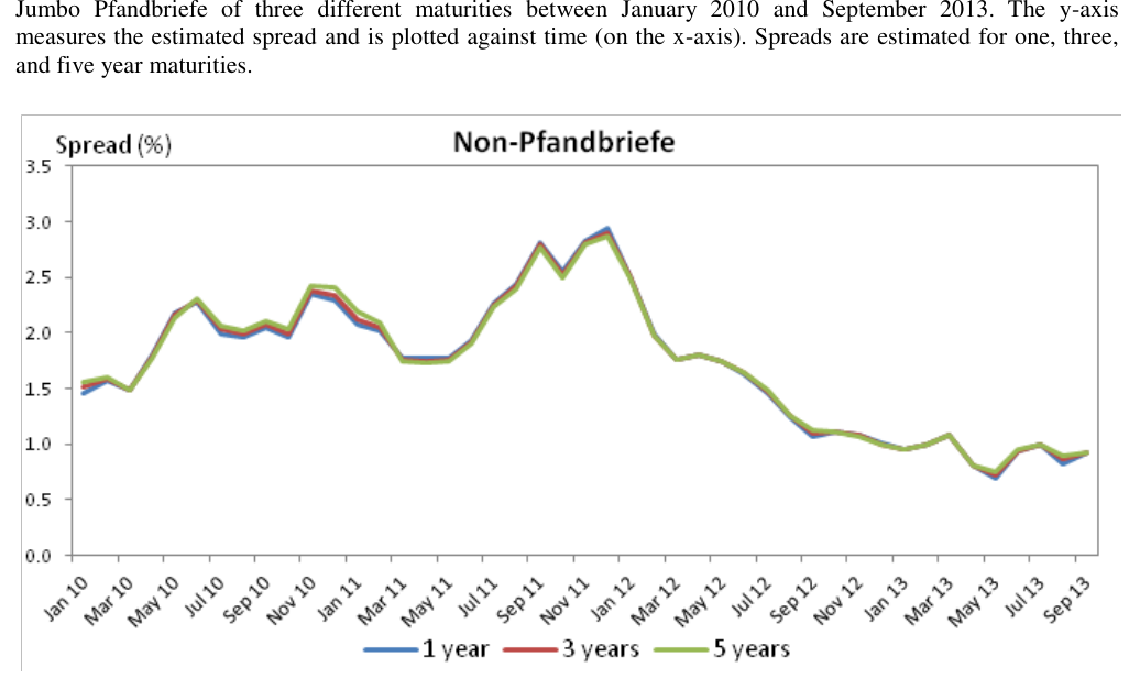
Figures 12, 13 and 14 contain plots of spreads for AAA-rated Covered Bonds and ABS over our sample period. These are an intermediate output of our analysis but are still somewhat interesting as they show how spreads (reflecting both credit and liquidity discounts) evolved in these markets over the sample period. The Covered Bond spreads peak just before the Draghi intervention. Pfandbriefe spreads show an inverted term structure which is what one might expect when the market is concerned about a crisis that is viewed as short-lived. The non-Pfandbriefe spreads exhibit a much flatter term structure suggesting that risks were seen as longer lived.
Figure 12 - Pfandbriefe Spreads: This figure shows the estimated evolution of spreads for AAA-rated
Figure 14 - Non-Pfandbriefe Spreads: This figure shows the estimated evolution of spreads for AAA-rated
It is not straightforward to fit term structures for individual ABS sub-categories because of lack of data, so we focus only on Euro-denominated RMBS. Figure 15 shows time series plots of RMBS spreads for different maturities. Again, there is some progression of spreads in maturity and again the spreads peak around the time of the Draghi intervention although they show some volatility in the spring of 2012 before finally declining in the summer of that year.
Figure 15 - ABS Spreads: This figure shows the estimated evolution of spreads for AAA-rated Euro-
To extract estimates of the portion of spreads that is attributable to liquidity, for each security and for each month-end day in our sample period, we calculate the gap between the actual price of the security and the price implied when one employs the AAA-spreads estimated as just explained. This price gap may be seen as the price discrepancy between the actual security price observed in the market and the price the security would have if valued using the spreads employed by the market, on average, for securities of that rating and class.
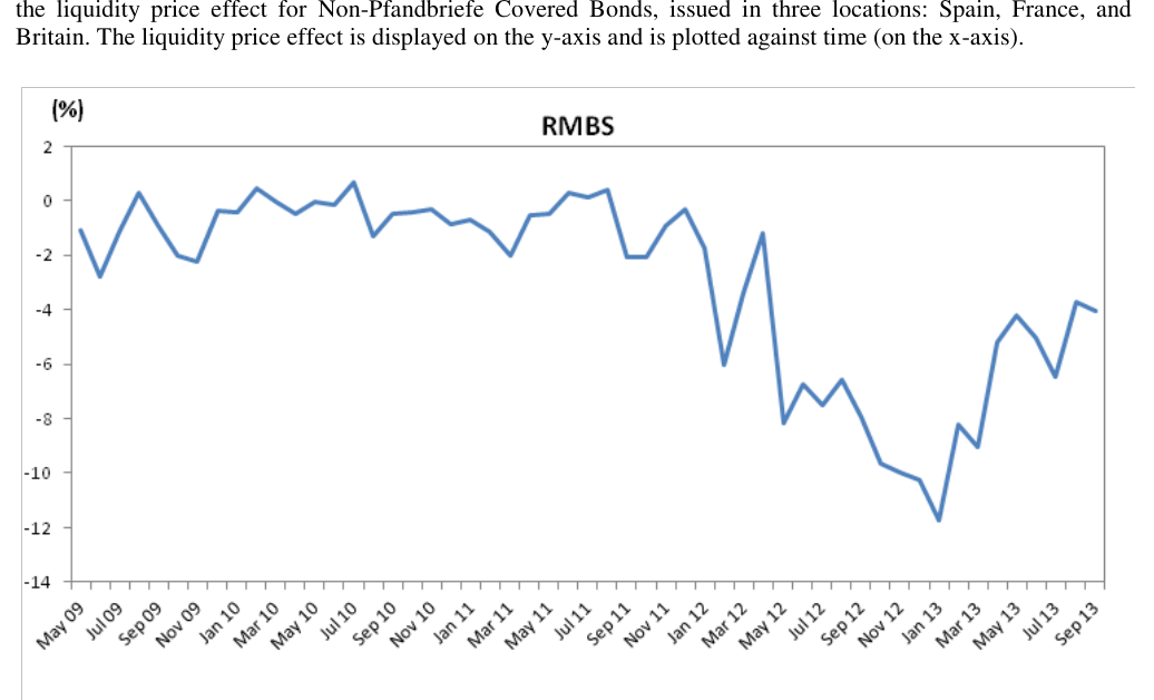
We then regress the price gaps on the bid-ask spread (as a measure of liquidity). The liquidity price effect is finally calculated by taking the product of (i) the resulting regression coefficient and (ii) the gap between the 10% and 90% quantile of the bid-ask spreads. This measure shows the discrepancy in pricing between high and low liquidity bonds. The approach we take (of performing regressions of gaps between market process and prices based on fitted spreads) effectively controls for both rating and maturity. Details of our approach may be found in Appendix 3.
Figures 16, 17 and 18 all show illiquidity effects over the sample period for Covered Bonds collectively, as well as for non-Pfandbriefe Covered Bonds and RMBS. The results in Figure 16 show substantial differences between Pfandbriefe (standard and jumbo) and other covered bonds. Again, the Draghi effect is very evident.
In Figure 17, we break down the non-Pfandbriefe results by country. The illiquidity discounts are greatest for Spanish securities. There is major volatility in discounts in the spring of 2011. The timing is different for France and Britain for which the peak discounts occur late in 2011.
The liquidity discounts for AAA-rated RMBS are substantial and similar in size to Spanish Covered Bonds. The emergence of liquidity discounts occurs later, however. We interpret this as showing that, as RMBS spreads narrow in 2011, the narrowing occurs first for liquid issues, causing a significant gap to open up between liquid and illiquid RMBS.
Figure 16 - Covered Bond Liquidity Price Effect: This graph shows the evolution over time of the liquidity
Figure 18 - Euro RMBS Liquidity Price Effect: This graph shows the evolution over time of the liquidity
SECTION 5 – CONCLUSIONS
This paper aims to provide a new perspective on the relative liquidity of two important European asset classes, Covered Bonds and ABS. We focus on evidence from bid-ask spread data, a data source neglected in the recent EBA analysis of asset class liquidity.
We present simple, transparent calculations of bid-ask spread distributions and then a more elaborate set of calculations that illustrate the contribution of market worries about future crisis-period transactions costs to individual security discounts.
Both approaches suggest that Covered Bonds and ABS are not as different as the EBA has claimed. The more liquid ABS exhibit greater liquidity than Covered Bonds do. In general, in the sovereign crisis period around 2011, Covered Bonds appear to have been less liquid than ABS. One category of short-dated, non-mortgage-related ABS, auto-loan-backed ABS, ranked very low for liquidity by the EBA, has tight spreads and so appears comparable to the most liquid Covered Bonds.
Taken together, we believe that our analysis suggests a different picture of the relative liquidity of asset classes than that presented by the EBA (2013b).
| Mean | Avg | Avg | Avg | Mean | Avg | Avg | Avg | |
|---|---|---|---|---|---|---|---|---|
| SD | 90% | 10% | SD | 90% | 10% | |||
| quant | quant | quant | quant | |||||
| Pfandbriefe | 0.32 | 0.16 | 0.51 | 0.12 | 0.35 | 0.13 | 0.52 | 0.18 |
| Jumbo Pfandbriefe | 0.20 | 0.11 | 0.34 | 0.09 | 0.25 | 0.10 | 0.36 | 0.14 |
| Other Covered Bonds | 0.40 | 0.18 | 0.66 | 0.19 | 0.44 | 0.19 | 0.72 | 0.22 |
| RMBS | 0.98 | 1.00 | 2.27 | 0.16 | 0.77 | 0.89 | 1.89 | 0.11 |
| CLO | 0.96 | 0.11 | 1.82 | 0.42 | 1.07 | 0.61 | 1.82 | 0.42 |
| CMBS | 0.97 | 0.83 | 1.75 | 0.18 | 1.03 | 0.88 | 1.82 | 0.14 |
| ABT | 0.58 | 0.29 | 0.91 | 0.28 | 0.61 | 0.31 | 0.93 | 0.29 |
| HEL | 0.65 | 0.49 | 1.27 | 0.10 | 0.47 | 0.39 | 0.99 | 0.04 |
| Auto Loan | 0.33 | 0.23 | 0.81 | 0.11 | 0.31 | 0.21 | 0.75 | 0.10 |
| Mean | Avg | Avg | Avg | Mean | Avg | Avg | Avg | ||
|---|---|---|---|---|---|---|---|---|---|
| SD | 90% | 10% | SD | 90% | 10% | ||||
| quant | quant | quant | quant | ||||||
| Covered Bonds (a) | Spain | 0.51 | 0.19 | 0.75 | 0.27 | 0.68 | 0.18 | 0.90 | 0.44 |
| France | 0.40 | 0.16 | 0.61 | 0.19 | 0.45 | 0.19 | 0.71 | 0.22 | |
| UK | 0.41 | 0.16 | 0.62 | 0.21 | 0.48 | 0.18 | 0.73 | 0.25 | |
| Italy | 0.37 | 0.11 | 0.51 | 0.22 | 0.62 | 0.18 | 0.75 | 0.34 | |
| Covered Bonds (b) | Spain | 0.58 | 0.16 | 0.76 | 0.35 | 0.68 | 0.15 | 0.83 | 0.45 |
| Italy | 0.54 | 0.11 | 0.67 | 0.37 | 0.73 | 0.14 | 0.83 | 0.47 | |
| RMBS (a) | Spain | 1.45 | 1.06 | 2.76 | 0.27 | 1.20 | 1.07 | 2.62 | 0.08 |
| Italy | 1.45 | 0.58 | 2.20 | 0.46 | 1.55 | 0.43 | 2.17 | 0.34 | |
| UK | 0.81 | 0.92 | 2.08 | 0.18 | 0.49 | 0.66 | 1.14 | 0.09 | |
| RMBS (b) | Spain | 1.40 | 0.92 | 2.49 | 0.34 | 1.24 | 0.85 | 2.28 | 0.31 |
| Italy | 1.34 | 0.78 | 2.31 | 0.47 | 1.34 | 0.78 | 2.36 | 0.43 |
Bibliography
Amihud, Yakov (2002) “Illiquidity and stock returns: cross-section and time-series effects,” Journal of Financial Markets, 5(1), January, pp.31-57, http://www.cis.upenn.edu/~mkearns/finread/amihud.pdf.
Australian Prudential Regulatory Authority (2013) “Discussion Paper: Implementing Basel III liquidity reforms in Australia,” APRA Discussion Paper, May, http://www.apra.gov.au/adi/PrudentialFramework/Documents/Implementing%20Basel%20III %20liquidity%20reforms%20in%20Australia%20-%20May.pdf.
Basel Committee on Banking Supervision (2013) “Basel III, the Liquidity Coverage Ratio and liquidity risk monitoring tools,” Bank for International Settlements, January, http://www.bis.org/publ/bcbs238.pdf.
Bao, Jack, Jun Pan and Jiang Wang (2010) “The Illiquidity of Corporate Bonds” The Journal of Finance, 66(3), June, pp. 911-946.
Beirne, J., Dalitz, L., Ejsing, J., Grothe, M., Manganelli, S., Monar, F., Sahel, B., Susec, M., Tapking, J., & Vong, T. (2011). The impact of the Eurosystem’s covered bond purchase programme on the primary and secondary markets. European Central Bank, January 2011. http://www.ecb.europa.eu/pub/pdf/scpops/ecbocp122.pdf
Brennan, Michael, Sahn-Wook Huh and Avanidhar Subrahmanyam (2013), “An Analysis of the Amihud Illiquidity Premium,” Review of Asset Pricing Studies, 3(1), July, http://northernfinance.org/2012/program/papers/84.pdf.
Buchholst, Birgitte, Jacob Gytelberg and Thomas Sangill (2010) “Liquidity of Danish Government and covered bonds: Before, during and after the crisis. Preliminary findings,” Danmarks Nationalbank Working Paper (70), September, https://www.econstor.eu/dspace/bitstream/10419/82357/1/636118274.pdf.
Bushman, Robert, Anh Lee and Florin Vasvari (2010) “Implied Bond Liquidity,” Working Paper, January, http://www.unc.edu/~leanh/WorkingPapers/BLV_9Feb10.pdf.
Chen, Long, David Lesmond and Jason Wei (2007) “Corporate Yield Spreads and Bond Liquidity” The Journal of Finance, 62(1), February, pp. 119-149.
Dick-Nielsen, Jens, Jason Gyntelberg and Thomas Sangill (2012) “Liquidity in Government versus Covered Bond Markets,” BIS Working Paper (392), November, http://www.bis.org/publ/work392.pdf.
Draghi, Mario (2011) “Introductory Statement to the Press Conference (with Q&A),” European Central Bank Speech, 8th December, http://www.ecb.europa.eu/press/pressconf/2011/html/is111208.en.html.
European Banking Authority (2013a) “Discussion Paper: on Defining Liquid Assets in the LCR under the draft CRR,” February, https://www.eba.europa.eu/documents/10180/42030/DP-on-defining-liquid-assets-in-the- LCR.pdf..
European Banking Authority (2013b) “Draft Reports on the impact of the LCR and on uniform definitions of liquidity under Article 509 CRR,” EBA presentation, October, http://www.eba.europa.eu/documents/10180/416332/Liquidity+public+hearing+30+October+ -+presentation.pdf.
European Banking Authority (2013c) “Report on appropriate uniform definitions of extremely high quality liquid assets (extremely HQLA) and high quality liquid assets (HQLA) and on operational requirements for liquid assets under Article 509(3) and (5) CRR”, December, https://www.eba.europa.eu/documents/10180/16145/EBA+BS+2013+413+Report+on+defini tion+of+HQLA.pdf.
European Banking Authority (2013d) “Report on impact assessment for liquidity measures under article 509(1) of the CRR,” December, http://www.eba.europa.eu/documents/10180/16145/EBA+BS+2013+415+Report+regarding+ LCR+impact.pdf.
European Central Bank (2011a) “6th October Press Release,” European Central Bank Press Release, October, http://www.ecb.europa.eu/press/pr/date/2011/html/pr111006_3.en.html.
European Central Bank (2011b) “3rd November Press Release,” European Central Bank Press Release, November, http://www.ecb.europa.eu/press/pr/date/2011/html/pr111103_1.en.html.
European Central Bank (2012) “31st October European Central Bank Press Release,” European Central Bank Press Release, October, http://www.ecb.europa.eu/press/pr/date/2012/html/pr121031_1.en.html
European Union (2013) “Capital Requirements Regulation,” 575/2013, June, http://eurlex.europa.eu/LexUriServ/LexUriServ.do?uri=OJ:L:2013:176:0001:0337:EN:PDF
Ewing, Jack and David Jolly (2011) "Banks in the euro zone must raise more than 200bn euros in the first three months of 2012," New York Times, December, retrieved 21st December 2011, http://www.nytimes.com/2011/12/22/business/global/demand-for-ecb-loans-surpassesexpectations.html?_r=0.
Fawley, Brett and Christopher Neely (2013) “Four Stories of Quantitative Easing,” Federal Reserve Bank of St. Louis Review, 95(1), pp. 51-88, January, http://research.stlouisfed.org/publications/review/13/01/Fawley.pdf
Finaninspektion (2012) “Finaninspektion’s regulation regarding requirements for a liquidity coverage ratio and reporting of liquid assets and cash flows,” November, http://www.fi.se/upload/90_English/30_Regulations/1_Regulatory%20code/2012/fs1206_eng .pdf
Financial Services Authority (2008) “Strengthening liquidity standards,” Financial Services Authority Consultation Paper, 08/22, October, http://www.fsa.gov.uk/pubs/cp/cp08_22.pdf.
Financial Services Authority (2009a) “Strengthening liquidity standards 2: Liquidity reporting,” Financial Services Authority Consultation Paper, 09/13, April, http://www.fsa.gov.uk/pubs/cp/cp09_13.pdf.
Financial Services Authority (2009b) “Strengthening liquidity standards 3: Liquidity transitional measures,” Financial Services Authority Consultation Paper, 09/14, June, http://www.fsa.gov.uk/pubs/cp/cp09_14.pdf
Financial Services Authority (2009c) “Strengthening Liquidity Standards: including feedback on CP08/22, CP09/13, and CP09/14,” Financial Services Authority Policy Statement, 09/16, October, http://www.fsa.gov.uk/pubs/policy/ps09_16.pdf.
Fitch Ratings (2013) “Criteria for Rating Securitizations in Emerging Markets,” June, http://www.fitchratings.co.jp/ja/images/RC_20130627_Criteria%20for%20Rating%20Securit izations%20in%20Emerging%20Markets_EN.pdf.
Harris, Lawrence (1990) “Statistical Properties of the Roll Serial Covariance Bid/Ask Spread Estimator,” Journal of Finance, 45(2), pp. 579-590, June.
Huang, Roger and Stoll, Hans (1997) “The Components of the Bid-Ask Spread: A General Approach,” The Review of Financial Studies, 10(4), Winter, pp. 995-1034, http://www.acsu.buffalo.edu/~keechung/MGF743/Readings/B6%20The%20components%20 of%20the%20bid-ask%20spread.pdf.
International Monetary Fund (2011) “Germany: Technical Note on the Future of German Mortgage-Backed Covered Bond (Pfandbriefe) and Securitization Markets,” IMF Working Paper, July, http://www.imf.org/external/pubs/ft/scr/2011/cr11369.pdf.
Longstaff, Francis, Sanjay Mithal and Eric Neis (2005) “Corporate Yield Spreads: Default Risk or Liquidity? New Evidence from the Credit Default Swap Market” The Journal of Finance, 60(5), October, pp. 2213-2253.
Mastroeni, Orazio (2001) “Pfandbrief-style products in Europe,” Bank of International Settlements (5), http://www.bis.org/publ/bppdf/bispap05b.pdf.
Moody’s Investors Service (2011) “Assessing the Impact of the Eurozone Sovereign Debt Crisis on Structured Finance Transactions,” April, https://www.moodys.com/researchdocumentcontentpage.aspx?docid=PBS_SF243137.
Office of the Controller of the Currency, the Board of Governors of the Federal Reserve System, and the Federal Deposit Insurance Corporation (2013) “Liquidity Coverage Ratio: Liquidity Risk Measurement, Standards, and Monitoring,” October, http://www.federalreserve.gov/aboutthefed/boardmeetings/FR-notice-lcr-20131024.pdf
Packer, Frank, Ryan Stever and Christian Upper (2007) “The Covered Bond Market,” BIS Quarterly Review, September, https://www.bis.org/publ/qtrpdf/r_qt0709f.pdf.
Roll, Richard (1984) “A Simple Implicit Measure of the Effective Bid-Ask Spread in an Efficient Market,” The Journal of Finance, 39(4), pp. 1127-1139, September, http://www.bauer.uh.edu/rsusmel/phd/roll1984.pdf.
Standard & Poor’s (2013a) “Request For Comment: Methodology And Assumptions For Ratings Above The Sovereign--Single Jurisdiction Structured Finance”, October.
Stirling, Craig and James Hertling (2011) "ECB Lends 489 Billion Euros for 3 Years, Exceeding Forecast," Business Week, December, retrieved 27th January 2012, http://news.businessweek.com/article.asp?documentKey=1377-aWQyiw0H4GIM- 497EEB4BELPRIE7TIUO0INS6SD.
Stoll, Hans (2000) “Friction,” The Journal of Finance, 55(4), August, pp.1479-1514, http://www.acsu.buffalo.edu/~keechung/MGF743/Readings/Friction.pdf.
Wookey, Jethro (2008) “ECB offers longer-term finance via six month LTROs,” Euromoney, May, http://www.euromoney.com/Article/1925778/ECB-offers-longer-term-finance-via-sixmonth-LTROs.html.
Appendix 1: bloomberg generic (bgn) and standard and poor’s bid-ask spread data
Bloomberg uses its own proprietary formula to calculate this bid-ask spread. This formula utilizes quotes provided by a proprietary set of contributors. The calculated bid-ask spreads are known as the Bloomberg Generic (BGN) bid-ask spreads and should be considered indicative not binding.
The definition of BGN provided by Bloomberg is as follow:
“The BGN pricing source is different than the Composite in that it does not just take the best bid/offer from selected contributors. Instead each contributor is assigned a quality score based on numerous factors including update frequency and spike frequency. The algorithm then uses this information to generate better prices and more accurate spreads. It also respects local market trading hours, this is because typical contributions outside of market trading are poor. We will always adjust these trading hours for particular currency pairs to be set for hours where we feel contributions are good.”
Bloomberg Generic Price (BGN) is Bloomberg's market consensus price for corporate and government bond. Bloomberg Generic Prices are calculated by using prices contributed to Bloomberg and any other information that we consider relevant. Bloomberg does not make a market in any of the securities that we price. The actual methodology we use is proprietary and depends on the type of pricing and the markets involved. The goal of the methodology is to produce "consensus" pricing. To the extent that we are not comfortable that a bond can be assigned a consensus price at any time, we will mark it "not priced". We constantly and vigorously review the performance of the system and alter it as we determine necessary to achieve our goal.”
BGN data has been used in a number of academic studies of liquidity, including, for instance: Bao, Pan and Wang (2010), Chen, Lesmond and Wei (2007) and Longstaff, Mithal, and Neis (2005).
The Standard & Poor's bid-ask spread data we employ is again based on a proprietary algorithm (including inspection and adjustment by analysts) that combines price quotes supplied to Standard & Poor's by multiple banks with the objective of obtaining market consensus bid and ask prices.
Appendix 2: spread term structure fits
This appendix provides information on the transition-matrix approach to fitting defaultable debt spread term structures for different ratings categories.
Consider a set of bonds with ratings from the set {1, 2, …, J} and prices , = 1, 2,…, N.
( )) ] ∑ [ (
where for j = 1, 2,…, are the cash flows of bond and the are the cash flows dates for j = 1, 2, …, .
Suppose that the dates are discretised so that the are all integers and that ratings evolve accordingly to a Markov chain with transition matrix[12] M. The transition matrix has the following shape:
( )
where denotes the probability of a bond moving from rating i to rating j in one year, for j, i = {1, 2, …, R}. The last column and row of the transition matrix M represent the probability of defaulting and it is denoted by for i = {1, 2, …, R}.
The default probabilities at horizons 1, 2, …, 30 years are the right hand column of powers of ( ) be the right hand column of the jth power of M, for j = {1, 2, …, 30}and for i = M. Let {1, 2, …, R}. The survival probability of a bond at time j conditional on rating i at time zero, ( ), is denoted as follows: denoted by ( ) ( )
Given a time homogenous transition matrix M, we can price a bond i as,
( )( )] ̃ ∑ [ ] [
Where γ is the expected recovery rate and it is constant across all rating categories; and is Treasury zero-coupon interest rate for a bond with maturity j.
If M is parameterized in a suitable manner, ( ̃), we can minimized the sum of the squared differences between the model and the observed prices over the vector ̃. To enforced appropriate properties for ( ̃), we parameterize it as:
( ̃ ) ̂ ( ̃ ) ̂ ( ̃ ) ( ̃ ) ( ̃ ) ̂ ( ̃ ) ̂ ( ̃)
( )
where,
( ̃ ) ̂ ( ̃ ) ( ̃ ) ̂
[̂ ] ∑ ( ̃ ) [ ]
Here, Φ(.) represents the cumulative standard normal distribution. We present the algorithm to estimate the parameters ̃ in the next section. The constraints for the problem are that the elements on the diagonal are less or equal to 1.
This approach to fitting term structures may be thought of as one of parameterising a ratingsbased credit derivative pricing model such as those of Jarrow, Lando, and Turnbull (1997) and Kijima and Komoribayashi (1998). These models assume that time-varying (rather than time-homogeneous, as in our case) ratings transition matrices are fitted to market price data and then the inferred risk-adjusted processes may be used to price more complex credit derivative contracts. In the context of this paper, we prefer to think of our approach as an interpolation technique for ordered credit spreads rather than as an implementation of a theoretical model.
Appendix 3: illiquidity discount effect estimation
This appendix explains how we estimate the illiquidity discount effect of traded bonds by studying the relation between price discount and bid-ask spread in a time-series fashion.
For a given trading day, we apply regression of price discount on the bid-ask spread as follow:
yi = β[0] +β[1]xi +εi
Here yi is the price discount (market price - model price) for bond i , and the face value of all bonds are assumed to be equal to 100;
xi is the averaged bid-ask spread of bond i over period between the adjacent price observation days. In this study we obtain price discount on a monthly basis therefore the bidask spread is constructed by averaging the daily bid-ask spread over the last one month;
β[0] and β[1] are the coefficients to be estimated;
To exhibit the difference between the pricing of bonds of high and low liquidity, we then obtain the low and high quantile value of the bid-ask spread, xi , and calculate the illiquidity discount effect, S, for a given day: ( ) : high quantile (e.g. 90%) value of xi ; : low quantile (e.g. 10%) value of xi ;
The regression analysis and discount effect calculation are conducted for all the observation days.
Note that one can segment bid-ask spread into different interested groups to obtain discount effect over different sub-samples.
Notes
[1] William Perraudin is a Director of RCL and Adjunct Professor of Imperial College, London. RCL was commissioned by the Association for Financial Markets in Europe (AFME), Prime Collateralised Securities (PCS) and certain AFME member firms to undertake the analysis set out in this paper. I thank Alexander Batchvarov, Alberto Ruiz-Sena and Rondeep Barua of BAML and Peter Jones, James West, Joseph Muck and Simon Collingridge of Standard & Poor’s for their comments and help in obtaining data. I also thank Richard Hopkin of AFME, Peter Nowell of BNP Paribas, Steven Gandy of Santander, Ian Bell of PCS, Fabrice Susini of BNP Paribas and Jim Ahern of Société Générale for their suggestions and insights. I thank Huaidong Wang, Thomas Wickstead and Susan Wu for their comments and assistance with different aspects of the calculations. The views expressed in this paper are my own and not necessarily those of any of the individuals or organisations mentioned above. Any errors remain my own responsibility. Correspondence should be addressed to the author at william.perraudin@riskcontrollimited.com.
[2] For a discussion of the key issues, see, for instance: European Banking Authority (2013b)
[3] If prices move randomly and one observes a random sequence of transactions at the bid and the ask price, then returns will tend to “bounce back”. The dealer buys at the bid price, which is low, and sells at the ask price, which is high. If one observes a high return in one period, it is likely that it involved a pair of prices successively at the bid and the ask prices. If the latest price is most likely at the ask price, the following one will be the same or lower so the next return will be negative. Hence, return data based on transactions prices is likely to exhibit negative autocovariances and the size of the autocovariance depends on the size of the bid-ask spread.
[4] Useful descriptions of the Covered Bond market may be found in Mastroeni (2001), Packer, Stever and Upper (2007), and International Monetary Fund (2011).
[5] The External Credit Assessment Institution (ECAI) system of credit grades may be summarised as follows. If two ECAIs provide ratings, the lower of the two is chosen. If three ECAIs rate the security, the second best is employed. The mapping from rating to ECAI grades is (using Standard & Poor’s notation) as follows: AA- and above is ECAI1, A- to A+ is ECAI2, BBB- to BBB+ is ECAI3, BB- to BB+ is ECAI4, B- to B+ is ECAI5, CCC+ and below is ECAI6.
[6] See Amihud (2002) and Brennan, Hu and Amihud (2013).
[7] See Roll (1984), Huang and Stoll (1997), Stoll (2000) and Harris (1990).
[8] A description of the proprietary algorithm used by Standard and Poor to calculate bid-ask spread data is given in Appendix 1.
[9] A description of the proprietary algorithm used by Bloomberg to calculate bid-ask spreads is given in Appendix 1.
[10] On the 8th of December 2011, Mario Draghi, President of the ECB announced a programme of Longer Term Refinancing Operations or LTROs (Draghi, 2011). These were loans with a three year term, 1% interest rate, and accepted loans from the banks’ portfolios as collateral. The total programme was announced for the sum of $640bn dollars or €489.2bn, an almost unprecedented intervention by the ECB. For market reaction, see, for instance: Ewing and Jolly (2011) or Stirling and Hirtling (2011). A useful overview of regulatory intervention in European markets over this crisis period, with a strong focus on intervention in secured debt markets (particularly, the Covered Bond market) is provided by Fawley and Neeley (2013).
[11] Note that the distributions for January and September 2013 in Figure 7 are for securities that were rated AAA in January 2012.
[12] The transition matrix is assumed to be in annual terms.