

The Simplified Supervisory Formula Approach (SSFA) is a simple, ad hoc approach to allocating capital across tranches with different seniorities. The SSFA has been adopted by the Basel authorities in their latest proposal (December 2013) as their formula-based approach for securitisation regulatory capital with a given calibration. In this paper, we present an alternative way to calibrate the SSFA that is more straightforward and transparent. This calibration is based on the rigorous, analytically solvable Arbitrage Free Approach (AFA) elaborated by Duponcheele et al. (2013a,b,c,d). In order to perform this calibration, we build upon the detailed investigation we have conducted on appropriate asset class-specific parameters for the Conservative Monotone Approach (CMA, a variant of the AFA). The CMA and its calibration are described in a sister paper, Duponcheele et al. (2014b). Our calibration has broader significance than simply the parameter values we obtain, in that we show how, by calibrating the SSFA for different regulatory asset classes, one may differentiate capital (across different parts of the securitisation market in a risk sensitive manner) without placing unrealistic information demands on investors. Last, we demonstrate how to achieve a much better fit between the capital charges implied by the SSFA and those implied by a more rigorous, model-based analysis such as the CMA. This can be done through a simple modification of the SSFA, by adding one additional parameter driving the 1250% risk weight threshold.
Executive Summary
This paper makes two contributions:
1. It presents a calibration of the Basel Simplified Supervisory Formula Approach (SSFA) using data and reasonable judgements. The Basel authorities’ calibration of the SSFA determines the parameter values of the -functions in both the regulatory securitisation IRBA and SA approaches (presented in the recent Basel consultative document BCBS (2013c)). The authorities performed their calibration using a substantially altered version of the Modified Supervisory Formula Approach (MSFA) described in a previous working paper, BCBS (2013a). Reportedly, the Basel authorities created a large number of stylised securitisation tranches and then found SSFA parameters that yielded capital similar to that implied by the altered version of the MSFA.
The approach to calibration proposed here is simpler and more transparent. We explicitly derive the SSFA parameter that matches the capital charge in the SSFA to that obtained from the Conservative Monotone Approach[3] (CMA), when subordination equals given multiples of the benchmark Basel capital level, or . We perform this exercise for a set of deals representative of different segments of the securitisation market using plausible and appropriate regulatory parameters[4].
The inputs to the SSFA are a single parameter, , the pool regulatory capital charge, and attachment and detachment points. The authorities have proposed two versions of the SSFA. i. The Standardised Approach (SA) version in which the pool capital charge ( ) is determined through the regulatory Standardised Approach (SA) for banking book exposures. The input of the formula, ( ), is obtained by adding (0.5- to where is the weight of delinquent assets in the pool. In this SSFA version the parameter is a constant, namely . ii. The Internal Ratings Based Approach (IRBA) version in which the pool capital charge is determined through the regulatory Internal Ratings Based Approach (IRBA) for banking book exposures. To this pool capital charge, one adds the one-year expected loss, to have ( ). In this SSFA version, has been defined as a linear function of deal characteristics (in particular but also pool type (wholesale or retail), pool loss given default, pool granularity, tranche maturity and tranche seniority).
A significant drawback of the BCBS proposal is that in practice the IRBA securitisation version of the SSFA will be applicable only to originators. The reason is that the regulatory requirements for measuring both and the arguments of the linear function for are practically impossible for investors to achieve due to the informational requirements they entail. Hence, for the vast majority of the market[5] a quite undifferentiated and unreasonably simple approach, the SA securitisation version, will be the only formula-based option for calculating securitisation capital.
Within Europe, where a ratings-based approach will be permitted by the authorities (at least initially), bank investors are likely to depend almost exclusively on external ratings to determine capital charges with respect to their holdings both under credit risk and market risk rules. This outcome is inconsistent with the objective of reducing regulatory reliance on ratings adopted by the European authorities following the May 2009 G20 summit.
The paper is organised around a calibration exercise. In explaining this exercise, we present our views on appropriate parameter values for the SSFA. However the exercise has a wider scope, for we are convinced that in many aspects our approach does much more to foster the market for securitisation[6] than the approach and the calibration proposed by the BCBS.
The calibration we propose demonstrates how one may develop a more differentiated SA-style SSFA, usable by investor banks. We generate appropriate values for different, fully observable sub-sectors of the securitisation market based on regulatory asset classes (for example, shortdated and long-dated corporate, residential mortgage backed, etc.).
It is our view that an approach differentiating regulatory asset classes should figure above the External Ratings Based Approach (ERBA), in a way that is more consistent with the intentions of European authorities of reducing reliance on external agency ratings[7]. Moreover, this approach could be extended to the IRBA securitisation version and thus also open to originators, leading to a simplified, more unified hierarchy.
2. The second contribution that this paper makes is to propose a “tweak” to the BCBS SSFA which permits a much closer fit between the SSFA and genuinely model-based and rigorous capital charges.
This slight modification of the SSFA yields a new “supervisory formula” that (i) takes into account the IRB risk drivers of the existing SFA and proposed MSFA, (ii) possesses some of the capital arbitrage-reducing properties of the AFA, while (iii) keeping the visual simplicity of the SSFA. We call this variant the Modified Simplified Supervisory Formula Approach (MSSFA).
The SSFA relies on a single regulatory parameter, . It is required to serve many (too many) purposes at once: i. it smooths out the cliff effect that occurs to the right of the pool capital level of subordination, ii. it determines the allocation of capital across mezzanine and senior tranches, iii. it defines the level of capital charge non-neutrality, i.e., the ratio of capital charge for all tranches of a deal to the capital charge a bank would hold against the underlying pool assets (before any additional impact of the floor). As one might expect, trying to hit so many targets with one variable is very difficult.
We, therefore, suggest the following small modification to the SSFA. The capital surcharge before the floor (equal to in the SSFA) is obtained in the MSSFA as the difference of two parameters ( :
• is a capital arbitrage-reducing factor for mezzanine tranches,
• determines the tail behaviour of the capital distribution (in the same way as in the SSFA).
We have also looked at the risk sensitive inputs to the SSFA, and concluded that a small change to the IRBA and SA inputs would improve the risk sensitivity and applicability of the approaches. In particular, we use the following definitions: a. the non-delinquent pool capital prior to securitisation, b. the delinquent pool capital, and c. the delinquency ratio.
The arbitrage-reducing MSSFA definition closely resembles that of the SSFA in its standardised version and may be summarised as follows[8]:
( (
(
( ) ( (
1. , (
2. , ( ([( )] [( ) ( ])
3. , ( (
Calibration Methodology and Results:
To summarise, our calibration methodology and results are as follows.
We calibrate both the SSFA and MSSFA by matching for those approaches the capital charges for thin tranches to the thin tranche capital ( implied by the Conservative Monotone Approach (CMA). We do this at calibration points specified as multiples of the pool capital. Here, is defined by:
( ) ( ) √ ) ( ( √
is the weighted average pool loss-given default for the non-delinquent pool. is a maturity-dependent capital surcharge scaling factor representing expected loss (inclusive of a risk premium and adjusted for future margin income) and is the maturity-dependent conditional pool correlation.
Both and could be set by regulators for the Basel II regulatory asset classes based on either (i) regulatory classifications[9] prior to securitisation or (ii) some other sectoral classification that reflects regulators’ views on the importance of specific markets.
For low granularity levels, with being the number of effective exposures, the formula may be adapted by replacing where: ( , and by ( .
The calibration of the CMA is described in Duponcheele et al. (2014b) and Table 1 below contains the suggested calibrated parameters for different Securitisation Regulatory Asset Classes.
8 The full description is provided in Appendix 2. 9 BCBS (2006), paragraphs 215, 216, 217, 218, --, 243
The best solution to calculate securitisation capital charges would be to use the CMA with pool specific variables such as , , and as well as the inputs and in Table 1.
The second best solution would be to use the MSSFA. Using Table 1, the values of and may easily be calibrated using the equations[10]:
( ( ) ( ( ) and ( ( )
The third best solution would be to use a calibrated SSFA. Using Table 1, the value of may be straightforwardly calibrated using the equation:
( ( )
Alternatively, instead of using the above formulae, one could use look-up tables, for securitisation regulatory asset classes:
• Table 2 provides the one-parameter SSFA values;
• Table 3 provides the two-parameter MSSFA and values. Both tables could be used under the IRBA and the SA methodology.
| Securitisation Regulatory | Asset Class | (can be | replaced | |||
|---|---|---|---|---|---|---|
| by IRB | values) | Senior | Non-Senior | |||
| Granular Short Term | Bank/Corporate | 46% | 8% | 1.00 | 1.05 | |
| Granular Low RW | Medium to Long | Term | ||||
| 46% | 22% | 1.05 | 1.18 | |||
| Bank/Corporate | ||||||
| Granular High RW | Medium to Long | Term | ||||
| 46% | 16% | 1.10 | 1.36 | |||
| Bank/Corporate | ||||||
| Granular Small- and | Medium-sized | Entities | 45% | 15% | 1.05 | 1.17 |
| Specialised Lending | (Commodities | Finance) | 27% | 13% | 1.00 | 1.18 |
| Specialised Lending | (Project Finance) | 27% | 33% | 1.10 | 1.33 | |
| Specialised Lending | (Object Finance) | 27% | 27% | 1.16 | 1.52 | |
| Specialised Lending | (Income Producing | |||||
| 47% | 36% | 1.06 | 1.19 | |||
| Real Estate) | ||||||
| Specialised Lending | (High Volatility | |||||
| 47% | 34% | 1.08 | 1.24 | |||
| Commercial Real | Estate) | |||||
| Other Granular | Wholesale | 76% | 30% | 1.07 | 1.23 | |
| Other Non-Granular | Wholesale | 53% | 40% | 1.08 | 1.26 | |
| Low RW Residential | Mortgages | 25% | 11% | 1.14 | 1.47 | |
| High RW Residential | Mortgages | 45% | 12% | 1.22 | 1.73 | |
| Revolving Qualifying | Retail | 75% | 3% | 1.06 | 1.39 | |
| Other Retail | 75% | 12% | 1.10 | 1.35 |
| Senior | Non-Senior | ||
|---|---|---|---|
| Securitisation Regulatory | Asset Class | ||
| Granular Short Term | Bank/Corporate | 0.27 | 0.29 |
| Granular Low RW | Medium to Long | ||
| 0.47 | 0.54 | ||
| Term Bank/Corporate | |||
| Granular High RW | Medium to Long | ||
| 0.36 | 0.52 | ||
| Term Bank/Corporate | |||
| Granular Small- and | Medium-sized | ||
| 0.43 | 0.49 | ||
| Entities | |||
| Specialised Lending | (Commodities | ||
| 0.21 | 0.28 | ||
| Finance) | |||
| Specialised Lending | (Project Finance) | 0.55 | 0.69 |
| Specialised Lending | (Object Finance) | 0.50 | 0.77 |
| Specialised Lending | (Income | ||
| 0.55 | 0.62 | ||
| Producing Real Estate) | |||
| Specialised Lending | (High Volatility | ||
| 0.52 | 0.62 | ||
| Commercial Real | Estate) | ||
| Other Granular | Wholesale | 0.54 | 0.62 |
| Other Non-Granular | Wholesale | 0.58 | 0.67 |
| Low RW Residential | Mortgages | 0.44 | 0.66 |
| High RW Residential | Mortgages | 0.44 | 0.89 |
| Revolving Qualifying | Retail | 0.23 | 0.41 |
| Other Retail | 0.46 | 0.61 |
| Senior | Non-Senior | ||||||
|---|---|---|---|---|---|---|---|
| Securitisation Regulatory | Asset Class | ||||||
| p2 | p1 | (p2-p1) | p2 | p1 | (p2-p1) | ||
| Granular Short Term | Bank/Corporate | 0.34 | 0.28 | 7% | 0.37 | 0.26 | 11% |
| Granular Low RW | Medium to Long | 26% | |||||
| 0.77 | 0.64 | 13% | 0.85 | 0.58 | |||
| Term Bank/Corporate | |||||||
| Granular High RW | Medium to Long | ||||||
| 0.47 | 0.31 | 17% | 0.63 | 0.22 | 41% | ||
| Term Bank/Corporate | |||||||
| Granular Small- and | Medium-sized | ||||||
| 0.65 | 0.54 | 12% | 0.73 | 0.49 | 25% | ||
| Entities | |||||||
| Specialised Lending | (Commodities | ||||||
| 0.25 | 0.19 | 6% | 0.32 | 0.14 | 18% | ||
| Finance) | |||||||
| Specialised Lending | (Project Finance) | 0.98 | 0.78 | 20% | 1.16 | 0.69 | 47% |
| Specialised Lending | (Object Finance) | 0.73 | 0.47 | 26% | 1.03 | 0.35 | 69% |
| Specialised Lending | (Income | ||||||
| 1.06 | 0.93 | 13% | 1.16 | 0.87 | 29% | ||
| Producing Real Estate) | |||||||
| Specialised Lending | (High Volatility | ||||||
| 0.90 | 0.72 | 18% | 1.03 | 0.65 | 37% | ||
| Commercial Real | Estate) | ||||||
| Other Granular | Wholesale | 1.01 | 0.88 | 13% | 1.12 | 0.81 | 31% |
| Other Non-Granular | Wholesale | 1.17 | 1.00 | 17% | 1.34 | 1.00 | 34% |
| Low RW Residential | Mortgages | 0.62 | 0.42 | 21% | 0.86 | 0.31 | 55% |
| High RW Residential | Mortgages | 0.56 | 0.29 | 28% | 1.03 | 0.16 | 88% |
| Revolving Qualifying | Retail | 0.27 | 0.18 | 9% | 0.44 | 0.09 | 35% |
| Other Retail | 0.73 | 0.57 | 16% | 0.90 | 0.48 | 42% |
Section 1 - introduction
The Basel Committee’s recently published proposals for securitisation regulatory capital[11] (see BCBS (2013c)[12]) include several approaches that place different informational demands on users. Unlike the previous proposals, for securitisation regulatory capital (see BCBS (2012)[13]), the approaches allocate capital to tranches of different seniority using a common mathematical function: the Simplified Supervisory Formula Approach (SSFA).
Finding its roots in the very first Basel working paper on securitisation capital (see BCBS (2001))[14], the SSFA was later developed and applied in the United States to calculate capital for securitisations held in banks’ trading books. The SSFA allocates capital to different tranches of a securitisation using a simple exponential smoothing function. Tranches for which the detachment point is less than attract capital equal to their par value. If a tranche has an attachment point is greater than , it is assigned a fraction of determined by an exponential smoothing function that allocates more to mezzanine than to senior tranches. The exponential weighting function employed is ad hoc and has no theoretical justification.
The authorities’ proposals envisage two versions of the SSFA. In the first, labelled the Internal Ratings Based Approach (IRBA), an input to the SSFA is , the level of capital an IRBA bank would calculate for the underlying asset pool (plus the one-year pool Expected Loss). In this case, the parameter in the SSFA is a linear function of deal characteristics. In the second version, referred to as the Standardised Approach (SA), the regulatory capital input to the formula is , the capital a Standardised Approach bank would calculate for the asset pool and is constant and equal to unity for all standard securitisations (not involving re-securitisation).
The hierarchy of approaches proposed by the Basel authorities places the IRBA formula at the top, followed by an External Ratings Based Approach followed by the SA formula. In practice, very few banks (realistically only originators) will be able to employ the IRBA since no relaxation is envisaged by the Basel authorities in the strict informational standards that banks must meet in calculating . Hence, the vast majority of the market will be obliged to use the ratings based approach (if this is permitted). If there are no external ratings or if external ratings approaches are not permitted (as in the US), an investor bank will be obliged to use the SA. Hence, in practice, almost all the market in Europe will use the ratings based approach and correspondingly, almost all the market in the US will employ the SA.
This outcome appears very unattractive as the SA is extremely undiscriminating in its approach. After the recent sub-prime crisis, which began in a particular, widely-securitised asset class, employing a one-size-fits-all approach appears undesirable in the US. European authorities have announced their intention to follow the US in reducing reliance on agency ratings in regulatory applications; but the heavy use to which ratings will be put in calculating securitisation capital, will reinforce the role of ratings (contrary to announced policy objectives) and will leave only a one-size-fits-all approach (the SA version of the SSFA) as a possible future solution if permission to employ ratings were revoked in the future in Europe.
In this paper, we present calibration analysis of the SSFA using representative transactions corresponding to a set of regulatory asset classes. Our approach is much more transparent and less ‘black box’ than the one reportedly performed by the Basel authorities in calibrating the IRBA and
SA versions of the SSFA. Their calibration apparently consisted of (i) creating a large number of deals with underlying assets possessing a range of characteristics and with different tranche structures and then (ii) fitting the parameter as a linear function of deal and pool characteristics using a least squares criterion. We presume that the SA value of was deduced also from this exercise.[15]
The approach we employ here is much more straightforward in that we fit parameters exactly by matching the capital implied by the SSFA to that implied by an analytically solvable model, namely the Conservative Monotone Approach (CMA). This is a simple version of the family of models developed by Duponcheele et al. (2013a,b,c,d)[16]. The matching is performed for a level of capital equal to a multiple of the regulatory capital of the underlying pool. The resulting value of is a closed form expression depending on regulatory input parameters. Setting these input parameters to appropriate values for different asset classes, one may transparently obtain the values of that are appropriate for different sectors of the securitisation market.
While we present this analysis as a calibration exercise, it has broader implications and possible uses. Specifically, our analysis demonstrates an alternative way (compared with the authorities’ IRBA) of calibrating the SSFA so as to differentiate appropriately between different parts of the market. Instead of making a linear function of deal characteristics, one may set it to different levels that are broadly appropriate for securitisations corresponding to different regulatory asset classes. This permits differentiation of regulatory capital without requiring that users of the capital formula have unrealistically detailed information about underlying asset pools.
A second contribution of this paper is to consider minor extensions or modifications of the SSFA that are much better able to match the capital implied by a rigorous capital model, the CMA. The parameter carries a heavy burden in the SSFA in that it determines the allocation of capital between mezzanine and senior tranches, the capital surcharge for securitisation (i.e., the ratio of the sum of capital for all of the tranches to pool capital) and the steepness of the cliff effect in the region of subordination just above total pool regulatory capital. Hitting three targets with one parameter is an over-ambitious objective and, not surprisingly, SSFA capital departs significantly from what one could obtain from a more rigorously formulated model.
We therefore propose introducing a single additional parameter, slightly modifying and generalising the existing SSFA while leaving it visually simple (as regulators require). The extended SSFA is referred to as the Modified SSFA or MSSFA. We, again, apply our calibration approach of matching SSFA and CMA capital at subordination levels equal to multiples of the regulatory capital input, . We, again, do this for deals representative of different regulatory asset classes, obtaining a transparent, closed form calibration.
The calibration in this paper may be seen as an extension of work presented in Duponcheele et al. (2013b). In that study, we reviewed the history of the SSFA and compared it to the principles of the AFA as set out in Duponcheele et al. (2013a). We also demonstrated the link between the value of in the SSFA and the asset class concentration correlation[17] (or within pool correlation) of the AFA. Both parameters serve to determine the tail of the capital distribution, where senior tranches or senior mezzanines are normally structured. Interestingly, this enabled us to calculate a range for which the value is reasonable (from a correlation point of view) and a range for which the value is unreasonable.
The rest of the paper is organised as follows. Section 2 exposits and analyses the SSFA, discussing the regulatory choices embedded in this approach. Section 3 recapitulates the development of the AFA and its variant, the CMA, a rigorous risk model that can be calibrated using data. Section 4 shows how the SSFA, which is not a risk model, can be calibrated based on the CMA. Section 5 discusses the regulatory disadvantages of defining only one value of in the calibration of the SSFA, and proposes a way to reduce the arbitrage that is embedded in the SSFA while keeping its main advantages.
Section 6 discusses key differences between a securitisation exposure (tranche) and an underlying asset in a securitisation, emphasising how the risk characteristics of the former are affected by the fact that it is secured against an underlying portfolio. This section also discusses the key risk drivers of portfolio behaviour (conditional pool correlation, delinquencies, pool maturity, granularity). Section 7 is concerned with the structural effects on the capital of securitisation tranches, in particular with the definition of a tranche, and with the treatment of discounts and provisions on the tranches. Section 8 concludes.
Section 2: expositing the ssfa
In this section, we exposit key features of the SSFA as implemented in the SA proposed in the recent Basel consultative paper.
The key input for the SA version of the SSFA is , defined as 8% of the weighted average Risk Weights under the Standardised Approach (SA).
∑( ) ∑
(1)
As it enters the SSFA, is modified[18] by risk weighting the proportion, , of delinquent assets in the pool with a risk weight of 625% in the following way:
(2) ( ( (
In Duponcheele et al. (2013b), we discussed the history of the SSFA. In its initial version, the SSFA did not contain the notion of delinquency. The parameter was introduced following the recent financial crisis, in the SSFA used in US trading book regulations, to increase the risk sensitivity of the formula. This was clearly necessary as the pool risk weight of 35% or 50% was too low for US subprime assets in the absence of other adjustments. The parameter offered a simple way of correcting this deficiency, bringing the overall pool risk weight to a value in excess of 100% for the worst subprime deals. (Subsequently, US regulations began differentiating between two categories of residential mortgages, one attracting a risk weight of 50% and the other a risk weight of 100%.)
Reflecting regulators’ desire to be extremely conservative for junior tranches, the SSFA specifies that if the detachment point, , of a tranche is below a threshold, denoted , then the risk weight of that tranche is set to 1250%. In the SSFA, the standard approach sets this threshold equal to :
(3)
This feature of the capital formula is often referred to as the Basel II SFA requirement of “deduction below ” when is set to . This is because in previous regulations, banks had the choice between “deduction of capital” or risk-weighting at “1250%”.
In fact, credible and rigorous risk models do not generate deduction of this type. If capital is based on unexpected loss (as are the capital charges for on balance sheet loans under Basel II IRBA), capital should actually decline as the tranche becomes extremely junior. Even capital based on Marginal Value at Risk (Unexpected Loss plus Expected Loss) implies capital less than a full deduction for tranches in the neighbourhood of or . Since this 1250% risk-weight requirement makes regulatory capital depart far from economic capital, it and the cliff effect in capital that it implies are the source of major capital arbitrage opportunities in practice, as we discuss further below.
For tranches with an attachment point greater than , capital is calculated using an exponential function. ( ) (4) ( (
Here, the parameter is the lower boundary, defined as the distance from the attachment point and the 1250% threshold , and the parameter is the upper boundary, defined as the distance from the detachment point and the 1250% threshold :
(5) (6)
The parameter is defined as: (7)
One may show that the parameter equals the percentage of capital, , that is allocated to all tranches with attachment points above the threshold, .
The 2012 Basel Committee consultation document, BCBS (2012), describes as a “supervisory adjustment factor in the SSFA intended to reduce cliff effects and apply conservatism for tranches with detachment points beyond . In addition, the supervisory adjustment factor can be seen to account for imprecision or uncertainty associated with using standardised approach risk weights for underlying exposures in calculating .”
The more recent consultation document, BCBS (2013c), defines in a more transparent manner: “In the SSFA, the supervisory adjustment factor “ ” represents the relative capital surcharge for all securitisation exposures compared to the capital requirement for the underlying pool. In other words, the “ ” parameter is a ratio determined as follows:”
( ) ( )
( )
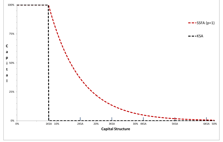
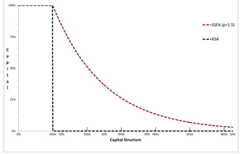
The cliff effect issue is illustrated by Figures 1 to 4, for a portfolio of 3-year BBB corporate exposures ( , i.e., ; 1-year ).
As is well-known, in an asymptotic single risk factor model of the kind used in the derivation of Basel II on balance sheet loan capital charges (see Gordy (2002) and BCBS (2005)), the Marginal Value at Risk capital for thin tranched exposures to a pool of loans equals 100% for junior tranches before jumping down to zero past a certain subordination point. This means that capital for thin securitisation tranches is a step function, as shown in Figure 1. (Note that a thin tranche just below or attracts 100% capital (i.e., 1250% RW), whereas a tranche just above or attracts 0% capital (i.e., 0% RW).) This is the cliff effect: a sudden change from 1250% RW to 0% RW occurring as seniority increases.
To smooth the allocation of capital and to generate strictly positive capital for senior tranches, different approaches have employed a range of assumptions (including attachment point uncertainty in the case of the Basel II SFA and conditional pool correlation in the case of the AFA).
The SSFA, however, is a non-model-based approach in which the degree of smoothing is determined by the value of the parameter in the exponential function. Figure 2 shows the effect of this smoothing with . Figures 3 and 4 demonstrate the effects of increasing the parameter to as proposed in BCBS (2013c) and as proposed previously in BCBS (2012).
For a tranche straddling the 1250% threshold, , i.e., for which the attachment point is below the 1250% threshold and the detachment point exceeds , the following formula in equation (8) is applied.
( ( ) ) ] (8) ( [( )] [( ) (
The formula in (8) ensures continuity of the capital distribution function for tranches in the region of . By setting the 1250% threshold so that: , equations (5) and (6) become:
(9) (10)
Finally, the definition of in equation (9) is replaced by the following:
(11) (
For the special case of a tranche straddling the threshold , we have . Since[19] , equation (8) can be rewritten as:
(12) ( [( )] [( ) ( ]
To summarise, we have as a formulation for the regulatory SSFA:
(13) ( ( ( )
( ( ) (
1. , (
2. , ( ([( )] [( ) ( ])
3. , ( (
The BCBS (2013c) proposals place the Internal Ratings Based Approach (IRBA) version of the SSFA at the top of the hierarchy for securitisation capital. The IRBA employs an SSFA capital allocation function with a parameter that is itself a function of various pre-securitisation IRBA parameters such as (including 1-year expected loss) and the pool . It also depends on pool granularity (reflected by the number of effective exposures ), and the maturity of the tranche, .
The supervisory parameter in the context of IRBA SSFA is defined as follows. As a first step, a parameter is determined: (14)
The linear coefficients , , , , and are given in Table 4 and depend on tranche seniority and the granularity of the asset pool.
Then, the parameter is restricted to take values in excess of in that:
(15) (
Figures 5 and 6 show the sensitivity of (for the senior tranche, granular pool, wholesale category, with 50 effective exposures), to the key risk drivers in this approach, i.e., the pool capital (including 1-year expected loss) (expressed as pool ), the pool , and the tranche maturity
. The value in this wholesale calibration is in the range [0.30 – 0.60] for the large majority of the wholesale market ( ) and ( ) and ( ).
Figures 7 and 8 show the sensitivity of for the senior tranche of a retail transaction, to the key risk drivers, the pool capital (including 1-year expected loss) (expressed as pool ), the pool , and the tranche maturity. The value in this calibration is in the range [0.30 – 1.40] for the large majority of the retail market ( ) and ( ) and ( ).
A striking feature of the above figures is the instability of the retail which varies substantially as the tranche maturity, , changes. This is because, for retail pools, the coefficient E adds a capital surcharge of 24% of additional pool capital per tranche maturity-year. The wholesale calibration does not exhibit this extreme sensitivity as the coefficient E adds a capital surcharge of just 7% of additional pool capital per maturity-year.
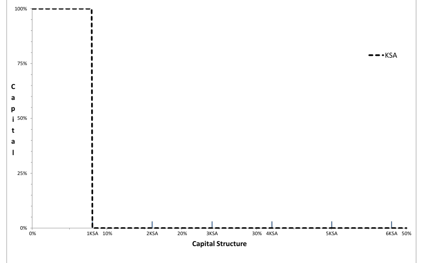
Note: The figure illustrates the “Cliff Effect” in that risk weights are 1250% below KSA and 0% above KSA.
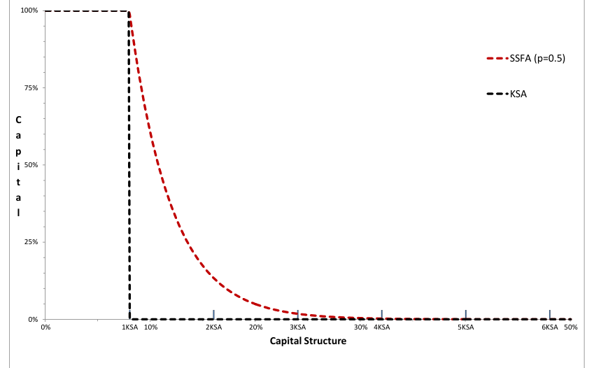
Note: The SSFA smooths the “Cliff Effect” with the parameter ‘ ’.
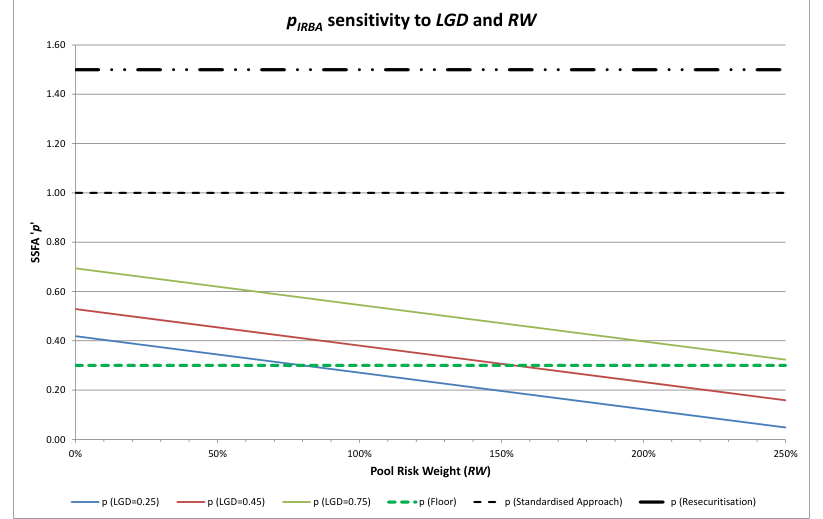
Note: Sensitivity to pool and pool ;
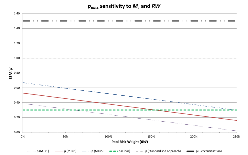
Note: Sensitivity to tranche and pool ;
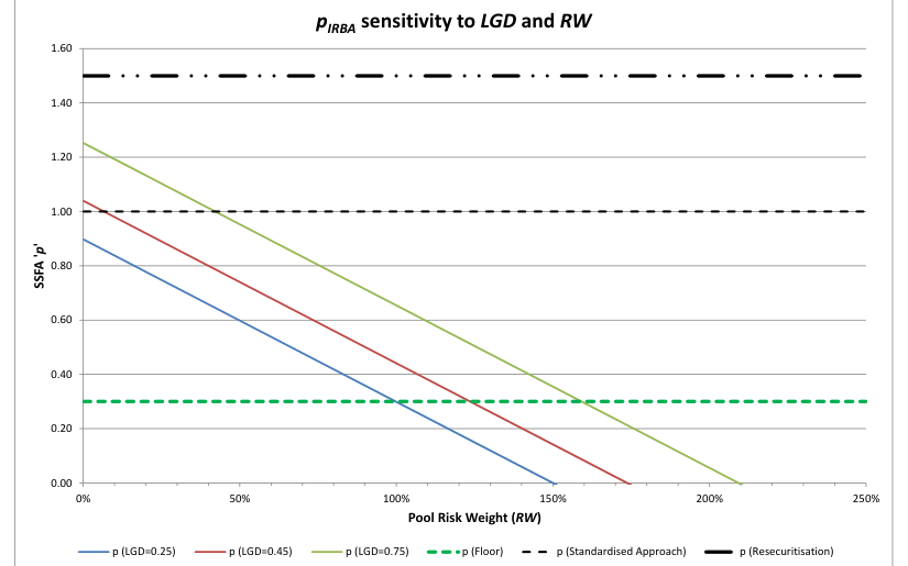
Note: Sensitivity to pool and pool ;
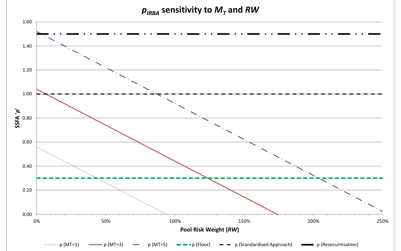
Note: Sensitivity to tranche and pool ;
| Coefficients | ||||||
|---|---|---|---|---|---|---|
| Tranche, Asset pool | ||||||
| for | ||||||
| ( Senior, Granular | 0 | 3.56 | -1.85 | 0.55 | 0.07 | |
| ( Senior, Non-granular | 0.11 | 2.61 | -2.91 | 0.68 | 0.07 | |
| Wholesale | ( Non-Senior, Granular | |||||
| 0.16 | 2.87 | -1.03 | 0.21 | 0.07 | ||
| ( Non-Senior, Non-granular | 0.22 | 2.35 | -2.46 | 0.48 | 0.07 | |
| Senior | 0 | 0 | -7.48 | 0.71 | 0.24 | |
| Retail | ||||||
| Non-Senior | 0 | 0 | -5.78 | 0.55 | 0.27 |
Section 3: the cma - a risk model calibrated from data
This section sets out the Conservative Monotone Approach (CMA). We will use this subsequently to calibrate the SSFA parameter, . In Duponcheele et al. (2013a), we develop a principles-based approach to securitisation capital, called the Arbitrage-Free Approach (AFA) using the same asset parameters as in the IRBA method prior to securitisation, i.e., , and systemic asset value correlation (AVC), together with a single additional parameter, the asset class concentration correlation, (now referred to as the conditional pool correlation).
Duponcheele et al. (2013b) derives the Simplified Arbitrage-Free Approach (SAFA) in which the inputs consist of the risk-weight alone (either IRBA or SA prior to securitisation) and other regulatory inputs such as the depending on the Standardised Approach asset type (and obtainable from simple look-up tables). We show that it is possible to determine the level of conditional pool correlation, , that is implicit in the SSFA parameter for a given attachment point, , by matching the thin tranche capital requirements between the SSFA and the SAFA.
Duponcheele et al. (2013c) also shows that maturity affects this conditional pool correlation, and that the marginal value at risk should be computed using a maturity adjusted correlation, . Duponcheele et al. (2013d) also demonstrates that the granularity parameter, , defined as the inverse of the number of effective exposures, , could be taken into account by employing correlation adjusted values. For very low granularity pools, they propose an additional adjustment to the lossgiven default.
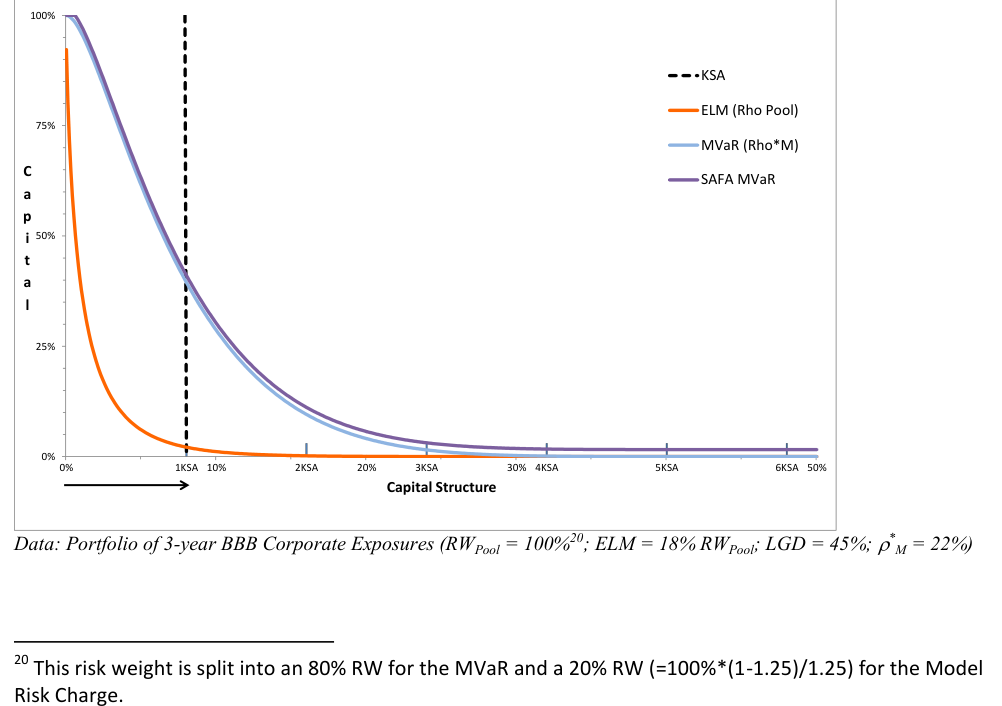
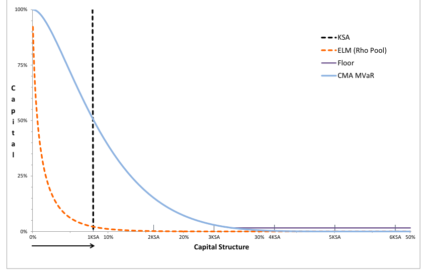
Graphically, the Unexpected-Loss capital for a tranche is the difference between the Marginal Valueat-Risk ( ) of that tranche (shown as the blue curve in Figure 9) and the Expected Loss at maturity ( ) of that tranche (shown as the orange curve in Figure 9), to which one adds a model risk charge (MRC) (shown as the purple curve).
In the AFA/SAFA framework, for the entire capital structure, the area between the MVaR curve and the ELM curve, plus the area between the MRC and the MVaR curve, equals the capital prior to securitisation. The AFA/SAFA in their original form enforces strict capital neutrality.
In our most recent work, we propose a variant of the SAFA, namely the Monotone SAFA, which departs from strict capital neutrality. This approach includes expected loss with a risk premium in the definition of capital so as to make the approach monotone.
Since the Expected Loss is not directly observed, we follow the approach within the Monotone SAFA of assuming it equals a maturity-dependent multiplier times the pool capital . We refer to the multiplier (plus one) as the Capital Surcharge Scaling Factor . Also, the SAFA model risk scaling factor is set so as to increase the amount of capital in the lower part of the capital structure, and the model risk charge is replaced by a floor requirement, making it thus conservative[21].
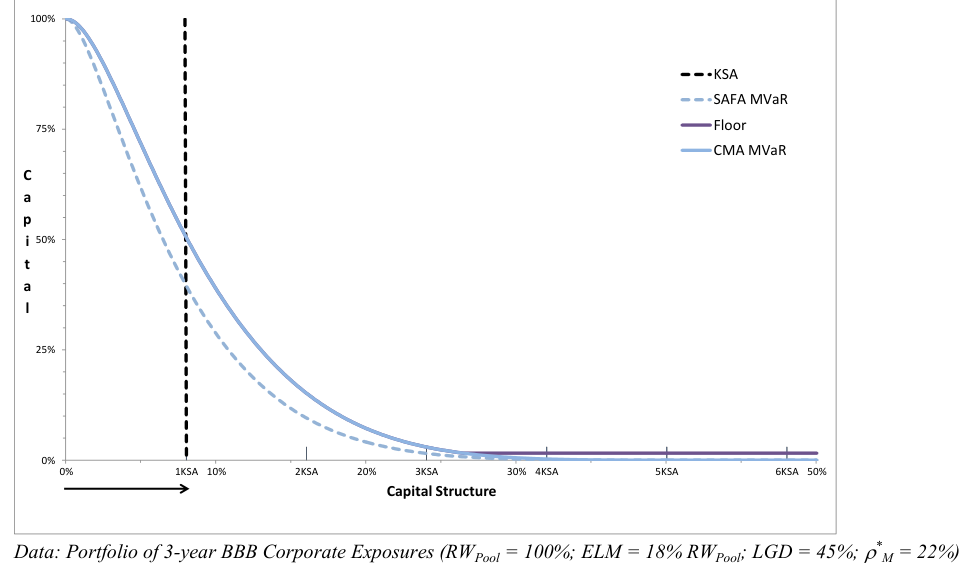
This SAFA variant that is both monotone and conservative is called the Conservative Monotone Approach (CMA). Figure 10 compares graphically the CMA and the original SAFA of Duponcheele et al. (2013b).
The thin tranche capital for the CMA may be expressed as:
( ) ( )√ ) (16) ( ( √
Here, is the Capital Surcharge Scaling Factor that, when multiplied with the capital of the pool, , equals the total amount of capital of all securitisation tranches compared to the asset pool capital, and the asset maturity, , is chosen when calibrating the parameters[22].
In this formulation, the capital of the pool can be defined, either using the IRBA definition which is the weighted average capital of the assets (excluding expected loss) as in IRBA multiplied by 1.06, or as its SA definition which is the weighted average SA risk weight of the assets multiplied by 8%. For pools comprising both IRBA and SA assets, can also be defined as the weighted average of and , to maintain consistency in the framework.
As long as the conditional pool correlation is different from 0%, the allocation of capital (Unexpected plus Expected Loss) of the CMA is done in a smooth way without a cliff effect, as shown in Figure 11, where it appears as an inverted S-shaped curve.
Because it is a credible and rigorous capital model derived from an analysis of underlying risk, the CMA may be calibrated using data. Here are some example calibrations (for non-senior tranches) for specific asset classes[23]:
• Short term corporate exposures: these are trade receivables, with maturities from 3 to 12 months. The risk weight of the trade receivables pool equals 100% under the Standardised Approach. The asset maturity, , may be set to 1 year (the regulatory minimum in Basel II). The maturity-dependent conditional pool correlation, , is calibrated at 8%. The 1-year expected loss after taking into account future margin income effect (expressed on the risk weight scale) is calibrated at 5% of the pool risk weight, thus the maturity-dependent capital surcharge scaling factor, , is set at 1.05. The loss-given default, , is set at 45%, as in Basel Foundation IRBA.
• Long term corporate exposures: these consist of corporate loans with maturity at origination greater than 1-year. The Basel II calibration of capital charges for loans was performed, reportedly, assuming that bank loans to corporates a seasoned average life of 3 years. The asset maturity, , is thus chosen to be 3 years. The risk weight of the long term corporate pool is set 100% under the Standardised Approach. The maturity-dependent conditional pool correlation, , is calibrated at 22%. The 3-year expected loss after taking into account future margin income effect (expressed on the risk weight scale) is calibrated at 18% of the pool risk weight. The maturity-dependent capital surcharge scaling factor, , is, hence, set at 1.18. The loss-given default is set at 45%, as in Basel Foundation IRBA.
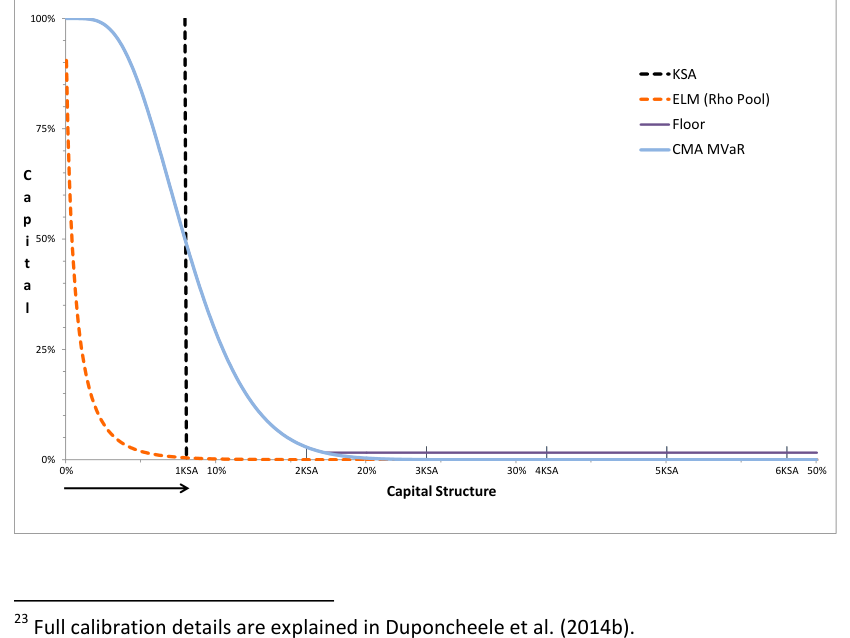
Figures 12 and 13 compare the capital implied by the CMA for deals involving short term corporate exposures such as trade receivables, and long term corporate exposures, respectively.
Both asset classes have the same risk weight; however, the maturity effect is noticeable. The asset maturity impacts the capital surcharge (1.05 and 1.18 respectively), which can be represented graphically as the area below the red dotted line.
The asset maturity also impacts the conditional pool correlation (8% and 22% respectively), whose effect can be seen in the tail behaviour of the capital distribution.
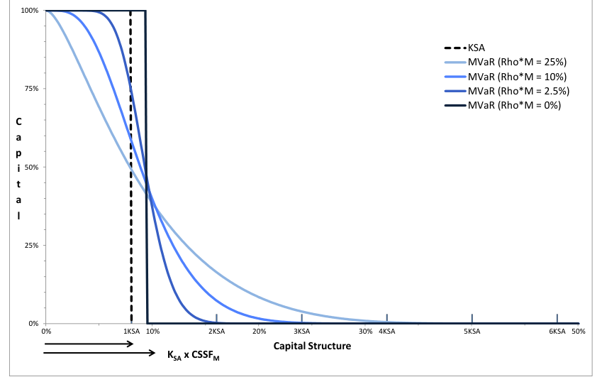
Note: Graph shows the Conservative Monotone SAFA (CMA) – Sensitivity to Conditional Pool Correlation. Data is for a portfolio of 3-year BBB Corporate Exposures (RWPool = 100%, i.e., KSA = 8%; ELM = 18% RWPool, i.e., CSSFM = 1.18; LGD = 45%; ρ*M = 0%, 2.5%, 10% and 25%)
| 100% | 1.05 | 8% |
|---|---|---|
| 100% | 1.18 | 22% |
Section 4: calibrating the ‘ ’ parameter of the ssfa
This section is concerned with the calibration of the ‘ ’ parameter in a way that is comparable to the exercises accomplished by the regulatory authorities in preparing BCBS (2013c).
Since both the CMA and the SSFA are monotone, one can compare them, highlighting, in particular, regions in which the SSFA overcapitalises or undercapitalises tranches compared to the CMA.
We are of the opinion that unnecessary overcapitalisation is likely to hamper the efficient operation of the securitisation markets and that undercapitalisation is not prudent from a regulatory point of view. The presence of both overcapitalisation and undercapitalisation will lead to arbitrage. We will revert to this point in the next section when proposing a way to modify the SSFA to reduce regulatory arbitrage.
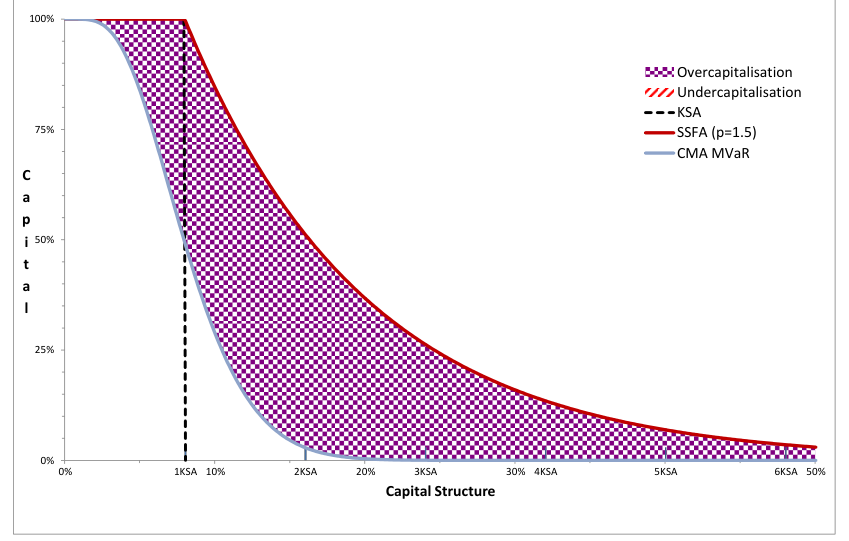
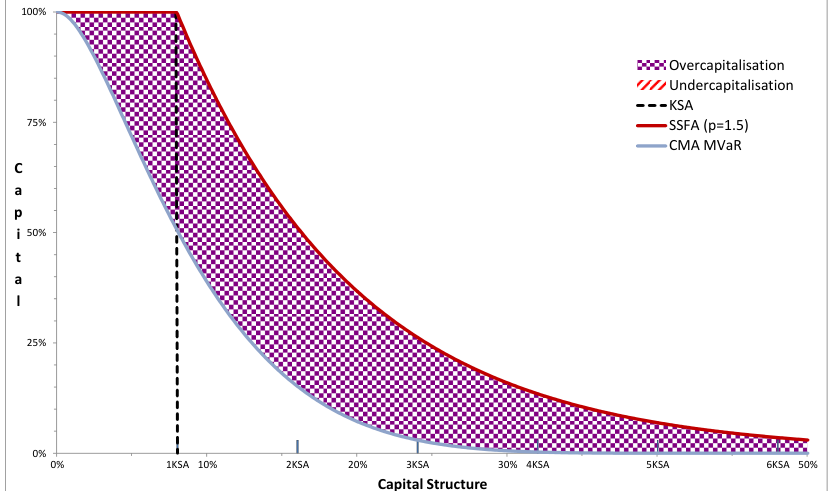
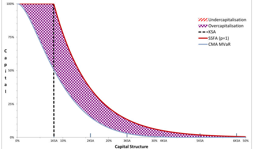
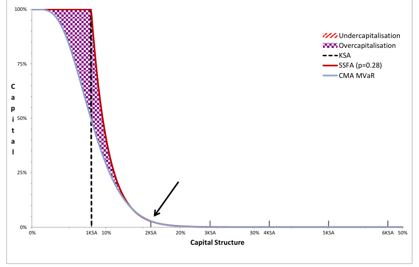
To start with, we will examine the SSFA as initially proposed in BCBS (2012) with a value of for securitisations other than re-securitisations. Figures 14 and 15 compare the capital implied by the CMA and the SSFA for deals involving trade receivables and long term corporate exposures, respectively. The very substantial degree of over-conservatism implied by a value of is apparent.
For this parameter value ( ), there is no level of seniority for which the implied capital level is even remotely close to the CMA capital which also appears in the figure. Note that this calculation of CMA capital is already significantly more conservative than on-balance-sheet capital since it is inclusive of expected loss with a risk premium, even when future margin income is taken into account.
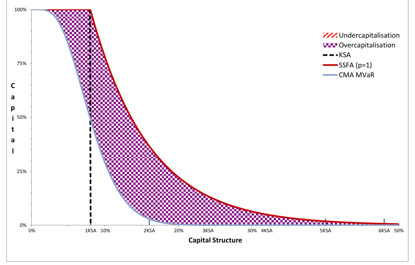
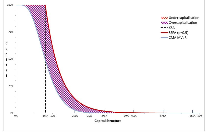
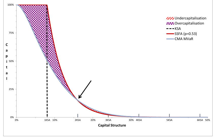
The SA version of the SSFA in BCBS (2013c) adopts the value: . Figures 16 and 17 show the capital implied by the CMA and the SA SSFA for trade receivables assets and long term corporate exposures, respectively. It is clear that this is an improvement compared to the BCBS (2012) proposals, but that the level of overcapitalisation is still excessively high, with severe distortion at the mezzanine level of the capital structure, in particular for short-term assets such trade receivables.
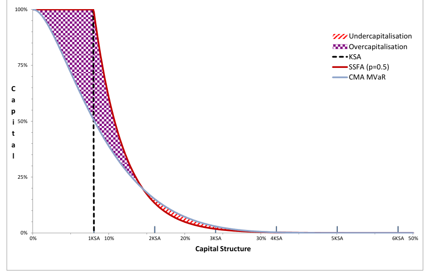
Figures 18 and 19 show the CMA versus the SSFA for trade receivables assets and long term corporate exposures respectively when , the current regulatory choice for US trading books. For short-term trade receivables, the shape of the SSFA capital curve is closer to that implied by the CMA, but still exhibits a layer of overcapitalisation compared to the CMA: a method which is already conservative. However, for long term loans, the SSFA curve intersects the CMA curve, leading to a junior portion of the capital structure which is overcapitalised and a senior portion which is slightly undercapitalised.
The comparison between short term corporate exposures and long term corporate exposures highlights that a single choice of the value for all assets classes in the SA SSFA of BCBS (2013c) is inappropriate.
There is already recognition in the IRBA version of the SSFA that the value should be a function of IRB risk parameters, such as pool capital, pool loss-given default, granularity, maturity and spread. There is also recognition that the value should be different for wholesale assets and retail assets.
This is a welcome differentiation, even though we consider that the retail asset class is not differentiated enough, as long-term retail exposures such as Residential Mortgages do not behave like short-term retail exposures such as Auto Loans or Credit Cards. This begs the question of how to calibrate the value in a more differentiated manner?
We have seen from the previous graphs that it is possible to compare directly the SSFA for a given value with the CMA of a given asset class. Nevertheless, there are constraints on both the SSFA and the CMA. The CMA allocates capital for all attachment points that are between 0% and the pool
24. The SSFA maintains 1250% up to a certain threshold , and then allocates the capital surcharge exponentially. So, there is a large mezzanine range, slightly above and slightly below (as both the SSFA and the CMA are monotone), in which there exists a value of such that at a given attachment point, the thin tranche capital of the SSFA will exactly match the thin tranche capital of the CMA.
When the attachment point is defined as a multiple of (such that ), the thin tranche capital of the CMA in equation (16) can be written as:
( ) ( )√ ) (17) ( ( ( √
In comparison, the thin tranche capital of the SSFA implies:
( ) (18) ( (
When the attachment point is defined as a multiple of , (i.e., ), equation (18) can be simplified as follows:
(19) ( ( (
To ensure consistency between the SSFA and the CMA, one may align thin tranche capital for particular values of the multiple, , by equating the two formulae, i.e.:
(20) ( (
Solving equation (20) with one calibration point defined as the multiple: , i.e., where the thin tranche capital of the SSFA is equal to the thin tranche capital of the CMA, by enforcing , yields the following result:
( (21) ( ( )
i.e. ( (22) ( ) ( )√ ( ( )) √
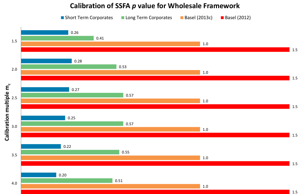
Table 6 below provides a numerical illustration of this value for both short term corporate exposures and long term corporate exposures, for different calibration values: . Calibration Short Term Corporate Exposures (Trade Long Term Corporate Exposures multiple Receivables and Trade Finance) (Corporate Loan Books) Value of Thin tranche capital Thin tranche capital Value of Value of (RW%) (RW%) 1.5 0.26 187.9% 0.41 364.8% 2.0 0.28 36.6% 0.53 191.3% 2.5 0.27 4.7% 0.57 90.5% 3.0 0.25 0.4% 0.57 37.7% 3.5 0.22 0.0% 0.55 13.2% 4.0 0.20 0.0% 0.51 3.5% Note: The CMA parameters are those in Table 5. The SSFA is set at ( ). No adjustment for granularity.
Figure 20 illustrates graphically the different values of , calibrated for the short term and long term corporate exposures. The values calibrated on data never come close to the proposed BCBS (2012) value of 1.5 (also shown on the graph), and even remain far away from the proposed BCBS (2013c) value of 1.0 (also shown on the graph).
Figures 21 and 22 show how the SSFA compares to the CMA if the calibration multiple of 2.0 is employed. The choice of a multiple is guided by the significance of the risk weight that is being calibrated for senior tranches.
One may observe from Table 6 that the implied value of is fairly stable with regards to the multiple for a given asset class, but varies widely across asset classes with about for short term corporate exposures and about for long term corporate exposures.
The value has a maturity dependency via the (the higher the maturity and the higher the risk weight, the higher the expected loss with a risk premium) and via the maturity dependency in the maturity-adjusted correlation: .
Comparison with the IRBA version of the SSFA in BCBS (2013c)
To compare with the IRBA version of the SSFA, consider the following values, , (i.e ), . Suppose we employ a maturity, , 1.0 for short-term corporate exposures and 3.0 for long-term corporate exposures[25].
For BBB short-term corporate exposures, equations (14) and (15) imply for senior tranches and for non-senior tranches. Since the approach imposes a floor, for seniors and for non-seniors. This is to be compared with for seniors and for non-seniors (Figure 21) when using a calibration multiple of .
For BBB long term corporate exposures we would have for seniors and for non-seniors. This is to be compared with for seniors and for non-seniors (Figure 22) when using a calibration multiple of .
Section 5: reducing ssfa arbitrage: a modified ssfa
The SSFA possesses 3 main advantages:
1. Using the Standardised Approach risk weights as the key input for the capital, , implies a level playing field for investors[26].
2. Visual simplicity, as the model employs a simple exponential function to allocate capital across tranches.
3. The approach is parsimonious in its use of parameters in that a single parameter controls the allocation of capital beyond the threshold .
But, the SSFA also has three fundamental drawbacks:
1. Oversimplification, due to the reliance on a single unique parameter, regardless of asset type and maturity, for radically different risk profiles.
2. The value of employed in US regulations of is a reasonably conservative calibration. The value adopted in BCBS (2012) of is excessively high. It is not possible to justify[27] such a value by inferring from a realistic value of . The value adopted in BCBS
(2013c) is for the SA SSFA, which is still too high and not justified for corporate exposures (where is around for short term corporate exposures and for long term corporate exposures). It is clearly not calibrated appropriately for retail exposures (where is between and depending on tranche maturity for the IRBA version of the SSFA).
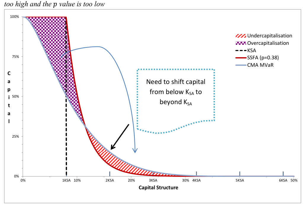
3. The choice of for the 1250% threshold implies substantial regulatory arbitrage opportunities. In the neighbourhood of the threshold, the capital of a thin mezzanine tranche equals 100% (i.e., a risk weigh of 1250%), whereas the unexpected loss, or even a Marginal Value at Risk inclusive of expected loss with a risk premium would be much less than 100%. This creates an arbitrage opportunity since by selling such tranches into the market, banks would reduce their capital by much more than is required to cover the risk. Investors price the risk of such mezzanines, tranched around the 1250% threshold, in line with the economic risk, which is materially lower than the price for first loss tranches (which have the same capital requirement). Thus, an inappropriate choice of the 1250% threshold creates a regulatory arbitrage opportunity. Figure 23 illustrates how to reduce this regulatory arbitrage, there is a need to shift capital from below the threshold to beyond it.
On the necessity of having at least 2 parameters and : the Modified SSFA
One may avoid overcapitalisation of the junior and junior mezzanines and undercapitalisation of senior mezzanines and seniors, if one employs instead two parameters and, correspondingly, two calibration points in fitting the exponential curve to the curve of the CMA. To achieve this, one may choose the parameters to ensure that a Modified SSFA exponential curve equals the CMA bivariate curve at two calibration points (corresponding to calibration multiples and ).
To achieve this, the 1250% threshold must be lower than , expressed with , in that:
(23) (
Beyond the 1250% threshold , one would allocate the capital using the exponential function with a parameter :
(24)
From (23) and (24), the total amount of capital is given by due to the 1250% threshold and , the sum of which is ( . So while in the SSFA, the capital surcharge (before any impact of the floor) is determined by the parameter , in the Modified SSFA, it depends on ( .
How might one calibrate the Modified SSFA parameters? One possibility would be to employ a least squares fitting approach for a set of stylised tranches and parameters. However, we think it is preferable to focus on areas of the tranche structure in which there are likely to be regulatory arbitrage opportunities.
Incentives to perform arbitrage related transactions reach their peak around (i.e., ), as this corresponds to the 1250% threshold whereas the Unexpected Loss is generally much lower. The parameter can thus be seen as a regulatory arbitrage-reducing parameter.
Another desirable feature of a calibration would be to ensure reasonably stable and accurate capital requirements for mezzanines. An appropriate calibration point for mezzanines would be at a point corresponding to 2 times (i.e., ).
Solving equation (20) gives:
( ( ) (
( ( ) ( ( )
( (25) ( ( )
Applying this equation at two values of the calibration multiple, and , one obtains:
( (26) ( ( )
( (27) ( ( )
Solving (25) and (26) gives closed form expressions for the parameters:
( ( ( ) ( ( ( ) (28) ( ( ) ( ( )
(29) ( ( ) ( ( )
For the special cases of and , the above equations simplify to:
( ( ) (30) ( ( ) ( ( )
(31) ( ( ) ( ( )
To summarise, by choosing[28] , one may eliminate the regulatory arbitrage opportunity at , and by choosing , one ensures that the differential between the Modified SSFA and the CMA is kept to a minimum for mezzanine tranches, while ensuring conservatism for the senior portion above .
In so doing, one ensures alignment of the Modified SSFA and the CMA, while retaining all the mathematical features of the SSFA.
Thus, the Modified SSFA (MSSFA) may be expressed[29] as:
(32) ( ( (
( ) ( (
1. , (
2. , ( ([( )] [( ) ( ])
3. , ( (
In the above formulae, we have picked out in red the (small) differences between the SSFA and the two-parameter version of the SSFA discussed here. In Table 7 and in Figures 24 and 25, we illustrate the effects of using the two parameter version of the SSFA.
Asset Class Value of capital Value of capital (RW%) (RW%) Short Term 0.25 617.8% 0.35 36.6% 0.10 Corporates Long Term 0.57 634.3% 0.83 191.3% 0.27 Corporates
Figure 24 shows capital for the Conservative Monotone Approach (CMA) and for the two-parameter Modified SSFA where the and parameters are calibrated on a 3-year BBB short term corporate exposures portfolio.
Figure 25 shows capital for the Conservative Monotone Approach (CMA) and for the two-parameter Modified SSFA where the and parameters are calibrated on a 1-year BBB long term corporate exposures portfolio. As may be observed, the fact that calibration has been effected at two points using two parameters substantially improves the consistency of the reduced form Modified SSFA and the CMA.
![Short Term Corporate Exposures: Modified SSFA (with p[1]=0.25 and p[2]=0.35) vs. CMA](/api/media/file/fig-1271.png?prefix=media)
![Long Term Corporate Exposures: Modified SSFA (with p[1]=0.57 and p[2]=0.83) vs. CMA](/api/media/file/fig-1272.png?prefix=media)

Section 6: portfolio behaviour in securitisation
One of the key differences between an asset which is a “securitisation exposure” (typically a tranche) and an asset which is a “securitised exposure”[30] (typically a loan) is the fact that a securitisation exposure will exhibit characteristics of portfolio behaviour whereas the securitised exposure will not. Thus, in order to model securitisation exposures accurately, the portfolio behaviour of the underlying assets of a securitisation must be considered.
Features of portfolio behaviour that are particularly relevant for capital calculations are:
• The conditional pool correlation, . This is a key component of the CMA. Duponcheele et al. (2013a) introduced this concept and Duponcheele et al. (2013c) gave it a maturity dependency.
• Provisions. From an accounting perspective, it is important to distinguish 2 key types of provisions that apply prior to securitisation: (a) “Loan Impairment”, also called Specific Provision, on an individual defaulted asset, and (b) “Collective Impairment” also called Portfolio Provision on delinquent assets, not yet defaulted[31]. We will see in section 6.A what these provisions imply for the factor employed in the SSFA and how a small change to the SSFA could significantly improve the consistency of the approach.
• Portfolio maturity. The true economic maturity of a securitisation exposure is affected by many factors including: (i) the underlying asset maturities (scheduled repayments), (ii) the prepayment on some assets (unscheduled repayments), and (iii) the recovery process on defaulted assets (driven by the legal system of the underlying assets). In section 6.B we will review the key issues with portfolio maturity and why the current tranche maturity definition in the IRBA SSFA changes the nature of this key risk driver.
• Portfolio yield. In a portfolio prior to securitisation, the entire yield (spread over a reference index or a reference risk-free rate after taking into account any swaps and senior costs) is available to offset expected loss. A senior tranche will benefit from such a yield, and sometimes will benefit more than other tranches due to interest diversion in securitisations’ payment priorities. However, a non-senior tranche will not benefit from the entire yield due to compulsory interest payments to the senior tranche. This is addressed in the calibration of the IRBA version of the SSFA by distinguishing the parameters A, B, C, D and E when determining the value for senior and non-senior tranches. However, there is no transparency in the calibration of these parameters. We will review in Section 6.C how this could be taken into account in a transparent manner.
• Portfolio granularity. We address this issue in Section 6.D.
Finally, Section 6.E summarises how Portfolio Behaviour is or is not taken into account in the different approaches: the MSFA, the IRBA version of the SSFA and the SA version of the SSFA, and discusses what could be done to improve consistency between these approaches.
Section 6.A: Portfolio Behaviour and Delinquency Ratio
Recent Basel proposals (BCBS (2012) and BCBS (2013c)) suggest improving the risk sensitivity of the SA version of the SSFA by adjusting the pool capital under the standardised approach, , by a factor “ ” representing the “delinquent” assets present in the pool, as per equation (33),
(33) (
This adjustment has the following implication for Risk Weights:
(34) (
While an improvement in the risk sensitivity of the standardised risk weight is welcome, one could ask whether the calibration risk weight of 625% is appropriate, and whether the adjustment leads to the intended result.
and 625%
To understand why an adjustment is needed, one may consider Principle 2 of the Arbitrage-Free Approach, the principle of neutrality. This suggests that one first analyses how provisions and capital for the asset pool are treated prior to securitisation and then what is required to generate consistent results after securitisation.
With the passage of time, a granular pool of performing assets will experience a credit migration with upgrades, downgrades and some defaults and losses. For the more serious deteriorations in credit quality (those leading to defaults and losses), the computation of capital requirements is not handled only by an increase in risk weights, but also by an interaction with accounting rules via the determination of provisions.
From an accounting perspective, prior to securitisation, there are two key types of provisions for the assets: (a) “Loan Impairment”, also called Specific Provision, on an individual “defaulted” asset, and
(b) “Collective Impairment” also called Portfolio Provision on “delinquent” assets, i.e., nonperforming assets that have not yet defaulted.
In BCBS (2012), “the variable would equal the ratio of the sum of any underlying exposures within the securitised pool that were “delinquent” to the ending balance. “Delinquent exposures” would be defined to mean exposures that were 90 days or more past due, subject to a bankruptcy or insolvency proceeding, in the process of foreclosure, held as real estate owned, had contractually deferred interest payments for 90 days or more, or were in default.”
The term “delinquent” in the Basel proposal does not have the same meaning as the one used in an accounting context. To make the link we need to split a pool of assets into three components: (i) performing, (ii) delinquent accounting-wise and (iii) doubtful accounting-wise. We may denote their respective weights in the pool, , and , as follows.
(35)
(36)
(37)
The capital under the Standardised Approach for the “performing” component is . The capital for “delinquent accounting-wise” component is , but an adjustment is made by the accountants by passing portfolio provisions. The portfolio provisions will be determined based on a statistical analysis of the proportion of assets in this category expected to move into the doubtful category in the near future: this is referred to as the “roll-rate”. The provision will converge to .
The category “delinquent accounting-wise” closely resembles the regulatory definition of “had contractually deferred interest payments for 90 days or more” in the regulatory definition of “delinquent exposures”. Such a definition would have created a major problem for some Southern European countries where the definition “had contractually deferred interest payments for 90 days or more” is a poor proxy for default, and for individual provisions. In other words, the ‘roll-rate’ of underlying exposures fitting only this part of the definition into future defaults is low for some asset classes in some countries.
The capital for the standardised approach for the “doubtful accounting-wise” component will converge to the sum of “individual impairments”, , and on the expected individual recoveries ( [32]. The category “doubtful accounting-wise” closely resembles the regulatory definition of “90 days or more past due[33], subject to a bankruptcy or insolvency proceeding, in the process of foreclosure, held as real estate owned, […], or were in default.”
Thus, prior to securitisation we will have for a pool capital:
(38) (
By setting (39)
we can compare this to the regulatory definition in equation (3), and assess the calibration of the implied risk weight for the regulatory “delinquent” assets.
Equation (40) requires an assessment of the meaning of the roll-rate for the different asset classes. However, BCBS (2013c) has changed the definition of the factor “ ”, to “the ratio of the sum of the amount of all underlying pool of exposures that are delinquent to the total amount of underlying exposures. The factor represents an uplift to take into account the deterioration of the underlying pool. The factor would be used to adjust and enhance the risk sensitivity” of the SA SSFA. It then states that “Delinquent underlying exposures are underlying exposures that are 90 days or more past due, subject to bankruptcy or insolvency proceedings, in the process of foreclosure, held as real estate owned, or in default.”
A technical improvement may be effected by not referring to “ending balance” for the denominator of the ratio, but to “the total amount of underlying exposures”. But more importantly, the reference to “had contractually deferred interest payments for 90 days or more”, is not present anymore. Therefore, the new regulatory definition in BCBS (2013c) of “delinquent exposures” is close to the accounting definition of “doubtful accounting-wise”.
Therefore, with this definition: (40) and
(41)
Equation (40) can be rewritten, in risk weight terms as in equation (42):
( ( (42)
For , equation (44) would become (45):
( (43)
For , equation (43) would become (44):
( (44)
This can be compared to equation (34), i.e,:
(45) (
We can see that this formula is calibrated reasonably for good quality retail assets ( ), recognising that the roll-rate of assets that are not-current (but not in default yet) should be taken into account.
In the case of higher LGD, such as corporate exposures or less good quality retail assets ( ), the risk weight of 625% is probably somewhat understated as the assets that are not current, but not in default yet, are not taken into account.
Overall, in the heavily simplified context of the SA version of the SSFA, a calibration of 625% for the regulatory “delinquent exposures” is broadly appropriate in the sense that it attempts to replicate the risk sensitivity in a pool prior to securitisation with the accounting implications on “doubtful” assets.
and the issue of the tail of the distribution
We have seen that is an important factor to improve the risk sensitivity of the SA version of the SSFA, as it replicates the interaction of accounting with capital prior to securitisation. Nevertheless, the issue of provisions in a pool prior to securitisation would affect only the junior tranches, and not the senior tranches. Provisions are not and should not be distributed.
However, a problem remains with the design of the SA version of the SSFA in that the tail of the distribution is affected inappropriately by the delinquency factor , as the parameter of the SSFA is a function of as in equation (46), which can be materially impacted by the term . In other terms the provisions are not just risk weighted at 1250%, they are also distributed to the senior tranches, and the problem is exacerbated with a high value of .
(46)
This can be addressed by modifying the parameter so that provisions only impact the junior part of the capital structure as in equation (37):
(47) (( )
And equation (47) could be simplified further in a conservative manner by equation (48)
(48)
Replacing equation (7) by equation (48) in the SA SSFA would be the only change required to address the delinquency ratio issue in the tail of the distribution.
Similarly, replacing equation (24) by equation (49) would be the only change required in a Modified SSFA to address both the delinquency ratio issue and the arbitrage-reducing concept described earlier. (49)
and the IRBA SSFA and CMA
The IRBA version of the SSFA does not have the concept of delinquency. In IRBA, doubtful underlying assets would impact the capital requirement . It is part of the 1250% threshold , and therefore this is analogous to . However, the delinquency should not affect the exponential part, as it would be equivalent to spreading provisions to senior tranches, and we have seen previously that in an arbitrage-reducing context, the 1250% threshold should be lower than .
One may improve consistency between the IRBA SSFA and the SA SSFA by defining two asset buckets: the regulatory ‘delinquent’ bucket with a ratio like in the SA SSFA with an IRBA capital and the ‘non-delinquent’ (performing) bucket with a ratio ( and a capital , such that:
(50) (
and since converges[34] to , we can write[35]:
(51)
A small modification in the IRBA SSFA could thus be obtained by setting the exponential parameter:
(52)
In an arbitrage-reducing context, the small modification to the IRBA SSFA could thus be obtained by setting the threshold:
(53) ( (
and the exponential parameter: (54)
Overall, aligning both IRBA SSFA and SA SSFA with the delinquency parameter would improve the consistency between both approaches, and enable the handling of mixed pools.
In a similar context, the CMA advocated by the authors would also benefit from the introduction of the regulatory parameter .
Section 6.B: Portfolio Behaviour and Tranche Maturity
For an individual loan (securitised exposure) prior to securitisation, the asset maturity definition in the IRBA wholesale framework is defined by (paragraph 320.a of BCBS (2006)):
∑ ( (55) ∑
“where denotes the cash flows (principal, interest payments and fees) contractually payable by the borrower in period .”
The current rules stipulate (paragraph 320.b of BCBS (2006)) “If a bank is not in a position to calculate the effective maturity of the contracted payments as noted above, it is allowed to use a more conservative measure of such as that it equals the maximum remaining time (in years) that the borrower is permitted to take to fully discharge its contractual obligation (principal, interest, and fees) under the terms of loan agreement. Normally, this will correspond to the nominal maturity of the instrument.”
When fees and interest payments are considered as a second order cash flow compared to the principal payments, equation (55) becomes the standard definition of a weighted average life (WAL) of an individual loan.
Most assets will fall under paragraph 320.a and therefore paragraph 320.b is rarely used.
The BCBS (2013c) proposals suggest the use of a similar definition for tranche maturity. Paragraph 23 of this consultative document stipulates: “For a securitisation exposure residing in a tranche subject to a determined cash flow schedule, tranche maturity ( ) is defined as:
∑ (56) ( ∑
where denotes the cash flows (principal, interest payments and fees) contractually payable by the borrower in period . The contractual payments must be unconditional and must not be dependent on the actual performance of the securitised assets. If such unconditional contractual payment dates are not available, the final legal maturity shall be used.”
Tranche maturity and portfolio behaviour
The previous wording for a tranche is unfortunate, as it neglects portfolio behaviour. We have seen how portfolio behaviour prior to securitisation has led to the introduction of the regulatory delinquency factor in the SSFA and of the conditional pool correlation in the modified MSFA. While we understand that keeping the same definition for maturity of a securitised exposure and a securitisation exposure creates the appearance of visual simplicity, this is incorrect as it renders the IRBA SSFA inconsistent by denying the effect of portfolio behaviour on effective tranche maturities for the large majority of asset classes (cash wholesale and cash retail).
Or more exactly, the only asset class that is properly modelled under the proposed tranche maturity definition are the synthetically referenced assets with bullet maturities; this is not a core activity of the securitisation market.
Portfolio prepayment impact: Most pools will experience some sort of prepayment. While the prepayment varies widely between asset classes (high for credit cards, low for auto loans, average for residential mortgages or for corporates) we understand that, short of a full internal model, it is difficult to use a ‘regulatory’ value of prepayment. However, experience shows that on average, in the banking system, it is possible to estimate the weighted average life of specific asset classes.
Portfolio performance impact: In the case of pass-through structures (the majority of the market), collected cash flows from the underlying assets are used to pay down principal on senior tranches and so the weighted average life of a tranche will depend on the performance of the assets.
Tranche maturity for real economy pools: a simple differentiation by asset class
The combined impact of portfolio prepayment, portfolio repayment and portfolio performance means that it is not just impractical but fundamentally incorrect to use the same regulatory definition for a tranche maturity as for an underlying asset maturity. Doing so fails to reflect appropriately the portfolio effect of this important risk dimension: maturity. We believe that it would be more sensible to calibrate a defined average pool maturity by taking a regulatory view on the key different asset classes. Having the right level of capital in the banking system as a whole (the prerogative of regulators) for the key asset classes is more important than trying to assess the exact riskiness of a specific transaction (the prerogative of an investor or rating agencies).
Granular Low RW Medium to Long Term Corporate Exposures 3.0 Granular High RW Medium to Long Term Corporate Exposures 3.0 Granular SME 2.5 Specialised Lending (Commodities Finance) 1.0 Specialised Lending (Project Finance) 5.0 Specialised Lending (Object Finance) 5.0 Specialised Lending (Income Producing Real Estate) 5.0 Specialised Lending (High Volatility Commercial Real Estate) 5.0 Other Granular Wholesale 5.0 Other Non-Granular Wholesale 5.0 4.0 Low RW Residential Mortgages 5.0 High RW Residential Mortgages 1.5 Revolving Qualifying Retail 3.0 Other Retail
Tranche maturity definition: a potential technical hidden barrier to trade within Europe
When structuring a securitisation, all arrangers will take into account the portfolio behaviour of the pool of assets in designing the liability structure. One technical point that arrangers need to address is the final legal maturity of the tranches. There are 3 key elements taken into account in this process: 1) the replenishment period[36] (sometimes called the reinvestment period), 2) the longest possible contractual cash flow in the pool of assets (based on covenants), and 3) the length of the judicial process in the jurisdiction where the assets are originated. The legal final maturity will be typically the sum of these 3 components.
While the first component is a risk factor and addressed in the Basel proposals (2013c), the second component exhibits portfolio behaviour and will diverge materially from the definition given in BCBS
(2006) for individual assets, and even more materially from the notion of weighted average life of the pool of assets.
The third component, the length of the judicial process is neutralised in the IRBA approach for the underlying assets, as the will be calculated as the amount of principal recovered, after full payment of unpaid interest during the work-out period[37]. In other words, for the same amount of recovery proceeds, the in a creditor friendly country such as the US or the UK will have higher IRBA than the in a not so creditor friendly country such as Italy or Portugal, as one will need to deduct a higher amount of interest payments, simply because the judicial legal process is longer in those countries.
The sentence in BCBS (2013c) “if such unconditional contractual payment dates are not available, the final legal maturity shall be used” means in effect that most securitisation tranches in the IRBA SSFA will use the tranche maturity based on the final legal maturity, capped at 5 years. Since the judicial legal process in Italy is commonly taken as being between 5 and 7 years, Italian assets, even very short term trade receivables, will always be assessed with a 5 year maturity, as the tranche legal final maturity will be far in the future. However countries such as the UK where the judicial legal process is commonly taken as being between 12 to 18 months, will benefit from lower levels of capital. This definition creates in effect a capitalisation not solely based on the risk parameters of the portfolio, but also creates a capitalisation on the basis of the length of the judicial process in a given country. Within Europe, this technical factor could well be considered as a hidden barrier to trade[38].
The proposed definition of tranche maturity in the IRBA SSFA disconnects the capital framework from the risk. Since the SA SSFA does not have a tranche maturity component in its definition, a calibration of tranche maturity for each broad category of asset class is a preferable route, as it would not discriminate de-facto against some countries and it would still make the framework risk sensitive to the important notion of maturity.
Tranche maturity: dealing with exceptions
There is one notable exception to Table 8. Some trading instruments, such as tranches on credit indices use the same fixed maturity for all the credit names present in the index. If there really is a need for trading books to have a maturity effect for those instruments, a central calibration could be done on a central value of 3 years and adjusted positively for longer maturities and negatively for shorter maturities, in a manner that is similar to what has been done in the BCBS (2013c) proposals. The legal final maturity for those instruments is not impacted by the legal judicial process of the countries whose assets are synthetically referenced as there is no real workout; instead the recoveries are cash settled following an auction process that normally takes place 3 months after default. Those trading instruments would benefit from the proposed tranche maturity definition and existing linear interpolation of tranche maturity in .
Section 6.C: Portfolio Behaviour and Future Margin Income
In the BCBS (2006) IRBA framework prior to securitisation, the unexpected loss is defined as the marginal value at risk less the one-year expected loss .
(57)
For the securitisation framework, however, the Supervisory Formula Approach (SFA) introduced a new variable, not the sum of the individual of all assets in the pool to make , but . The definition of in paragraph 627 of BCBS (2006) was “ is the ratio of (a) the IRB capital requirement including the EL portion for the underlying exposures in the pool to (b) the exposure amount of the pool”. The terminology “including” was translated into European law as “an addition” of the one-year expected loss of the pool to the unexpected loss. Therefore the relationship between , and can be described as:
(58) ∑
(59)
In essence, the introduction of expected loss into enabled the SFA to be monotone.
A similar concept, introducing the expected loss into the capital requirement to make the capital allocation monotone, is used in the MSFA and CMA, but over a longer maturity horizon: via the tranche maturity in the case of MSFA and asset pool maturity in the case of the CMA.
In the context of the CMA, the marginal value at risk , function of pool maturity , becomes:
(60)
As shown in Duponcheele et al. (2013c), can be calculated as:
(61) ( ( √ )
where is the probability of default[39] of an asset at maturity[40] and is the risk premium[41].
However, as shown in Duponcheele et al. (2013a), the introduction of long term expected losses into the capital requirement definition needs to be kept in check, to avoid changing the nature of what capital is supposed to cover.
In a portfolio prior to securitisation, the Future Margin Income or FMI (defined as the margin over a reference index or a reference risk-free rate) is designed to cover more than just the expected losses with a risk premium over the maturity of the portfolio. So a conservative financial view would be:
(62)
Prior to securitisation, in regulatory term, a full recognition of the FMI is given only up to the oneyear capital horizon[42]:
(63)
Beyond the one-year capital horizon, we should have:
(64)
Portfolio margin and senior tranches
In the securitisation framework, the capital definition is in fact a Marginal Value-at-Risk as it contains expected loss (to make the capital allocation monotone), and the BCBS (2013c) proposal proposes to recognise 80% of the FMI beyond the one-year horizon ( ), for senior tranches only. In a securitisation, there are costs (for example, rating agencies fees, administration fees, servicing fees, management fees, structuring fees and swap fees) which absorb some of the FMI, and therefore the value of 80% can be deemed both conservative and reasonable.
The FMI available to senior tranches is thus:
Therefore the marginal value at risk of the pool would be (for senior tranches)[43]:
(65) ( (
(
(
Portfolio margin and non-senior tranches
A key difference between the situations pre- and post-securitisation, vis-à-vis the issue of portfolio margins, is that the senior tranche will require payment of its coupons. Thus, for non-senior tranches, the FMI available is reduced by the amount of coupons payable to the more senior tranches. But this
40 The asset maturity to be used in this formula is the average asset maturity as in Table 8. 41 The Basel Working Paper 22 (BCBS (2013a), page 19) proposes a way to extract the risk premium, by applying the following equation √ 42 There is no reason to look beyond this one-year horizon, as banks are not closed pools. Securitised portfolios are closed pools, and expected losses over the life of the assets needs to be taken into account (as well as the FMI over the life of the assets). 43 This formulation is an approximation. For more details see Duponcheele et al. (2014b).
does not represent the entire margin since the very large majority of the non-senior tranches in the banking system receive coupons.
We estimate conservatively that 50% of the FMI available to the senior tranches will fall down the waterfall after senior coupon payments and be available to the non-senior tranches[44].
(66)
Therefore the marginal value at risk of the pool would be (for non-senior tranches):
(67) ( (
( (
(
Of note, the BCBS (2013c) proposals do not give even partial recognition of the FIM for non-senior tranches. This is overly conservative, as it implies that investors are not rational and will not require a higher margin on non-senior tranches compared to senior tranches. Applying a ratio of 0% in equation (66) is overly conservative, and as maturity increases, the capital as unexpected loss is overtaken by expected loss over the life of the assets. This would give the unreasonable (for long maturities) equation: ( .
Section 6.D: Portfolio Granularity
In the BCBS (2013c) proposals, the parameter, , in equation (14), uses the coefficient to handle the granularity , where is the number of effective exposures. This is only used in the wholesale framework. This makes sense, as there is no significant retail securitisation with very low granularity.
In the proposals, when , the contribution of the granularity to a senior tranche value is , i.e., a maximum of a 14.2% increase. This is not material and it would be better to simplify the calibration without this parameter, by assuming that asset classes are granular when , like in the retail framework.
However, when , the contribution is . So when there is only 1 asset which is tranched, is increased by at least 2.61. This multiplies the capital to such an extent that the cap will likely apply.
The CMA handles low levels of granularity by replacing with ( , and by ( . The CMA would not require the cap in the way the SSFA would, but would still allocate more capital to the senior tranche than if there were no granularity adjustment.
While low levels of granularity are more of an issue for specific trading instruments or unusual capital relief transactions than for real economy transactions, there is an exception for commercial mortgages backed securities (CMBS), where it is not unusual to have only one loan to an office property (e.g. a prime shopping mall or a prime office tower with many tenants). The real granularity in those transactions cannot be managed by a statistical desktop analysis. That is why we think that when calibrating, one must distinguish the CMBS category from Other Non-granular Wholesale securitisations - the risks are not the same.
Section 6.E: Portfolio Behaviour and Calibration Implication
The IRBA SSFA does differentiate between senior and non-senior tranches. This is achieved by distinguishing the parameters A, B, C, D and E when determining the value for senior and nonsenior tranches. This could be better calibrated by taking into account both the effect of portfolio yield and asset pool maturity for broad categories of regulatory asset classes. Below is a table summarising the issues discussed in this Section 6.
Conditional Pool Yes, directly, a 6% Yes, indirectly, via Yes, indirectly, via . value has been used. MSFA calibration. Correlation ( But is too high and should be differentiated by regulatory asset classes. Portfolio Delinquency No. No, this parameter is Yes, directly. The missing from the concept is correct and the risk weight formula. definition does not give associated with the adequate risk about right. However weight for defaulted implementation problems still exist in assets. , and the parameter . should be used instead. Portfolio Maturity Yes, but tranche Yes, via tranche No, this notion is maturity is not the right maturity, but the missing. It should be proxy for the risk on definition is taken into account by the asset pool. This inapplicable apart from different values of should be recalibrated specific trading per regulatory asset per regulatory asset instruments. The class. class, using the definition is also a maturity of the asset hidden barrier to trade pool. within Europe.
Portfolio Yield Yes, for senior tranches Yes, by distinguishing No, this notion is only. the coefficients , , , missing from the No, for non-senior and between senior calibration. There tranches. and non-senior should be tranches. differentiation between senior and non-senior tranches. Portfolio Granularity Yes. Yes, via the coefficient No. and the risk parameter .


Section 7: structural effects in cash securitisation
Section 6 was concerned with the impact of Portfolio Behaviour on the capital of securitisation tranches. This section, in contrast, is concerned with Structural Effects on the capital of securitisation tranches: in particular with the definition of a tranche, and with the treatment of discounts and provisions.
Key inputs to formula-based approaches to capital (that do not rely on external ratings), are parameters that describe the tranche structure. These include, for example, the credit enhancement ( ) and the thickness ( ) parameters used in the Supervisory Formula Approach (SFA) in BCBS (2006), or the attachment point ( ) and detachment point ( ) parameters employed in the MSFA, SSFA in BCBS (2012) and (2013c).
Implicit in these models is the assumption that capital reflects first order influences on risk including the principal outstanding of the underlying assets, but omits second order influences including the interest on the underlying pool assets, the default history of the pool, and the effects of costs or differences between the purchase price of assets and their exposure at default, and the book value of tranches and their exposure at default.
As such, these formula-based approaches to capital assume that the principal of all tranches will match the principal of all assets. In reality, a proper computation of a tranche’s credit enhancement or attachment point matters as the amount of principal on the liability side of an SPV does not necessarily match the amount of principal on the asset side of an SPV[45].
A proper definition of inputs helps in catering for the majority of transactions, but to avoid regulatory arbitrage, there is a need to have an overriding principle of regulatory prudence when the definition of the inputs is not adapted to economic realities. In this case, as illustrated below, the key principle is that tranche inputs should be in line with the economic substance.
Section 7.A: Attachment Point and Detachment Point
Definitions
Definition in BCBS (2006)
The BCBS (2006) definition for the credit enhancement ( ) is the following: “ is measured (in decimal form) as the ratio of (a) the amount of all securitisation exposures subordinate to the tranche in question to (b) the amount of exposures in the pool”. This definition is unsatisfactory, as the numerator of the ratio is not an assessment of how many assets are available to support the tranche (the traditional meaning of credit enhancement) but an assessment of the subordination of the tranche).[46]
• Example 1: a cash securitisation has USD 98m of assets and USD 100m of liabilities. Assume, that the senior tranche is USD 80m, the mezzanine tranche is USD 15m, and the junior tranche is USD 5m. The mezzanine tranche has a financial subordination of USD 5m (the size of the junior tranche), but a credit enhancement of USD 3m (the amount of loan assets remaining after redemption of the senior and mezzanine tranches). The literal application of the definition could create capital arbitrage opportunities to reduce the capital requirement artificially. Indeed, a literal application of the definition of the current BCBS
(2006) definition of the SFA means that the variable ( ) is 5.1% {= 5junior / 98assets} when it should be 3.1% {= (98assets - (80senior + 15mezzanine)) / 98assets}. It is down to banks with conservative risk management approaches to ‘interpret’ the principle behind the definition, to assume that the regulators meant ‘credit enhancement’ instead of ‘subordination’ and to use the correct value of 3.1% in their risk systems, instead of 5.1% which would result from the literal application of the definition.
The situation is exacerbated when the portfolio deteriorates, when assets have defaulted, resulting in losses. The literal application of the current BCBS (2006) definition improves the credit enhancement ( ) when losses have occurred, a result which is obviously economically incorrect:
• Example 2: using the same tranches as in the above example, assume that the portfolio of assets is now USD 90m following USD 8m of losses. The numerator of the ratio for the mezzanine tranche is still USD 5m, as the junior tranche of the securitisation still exists. The denominator is USD 90m. Therefore, the literal application of the definition means that is now 5.6% {= 5junior / 90assets}, an increase compared to the 3.1% when there were no losses! The financial credit enhancement would be in reality the negative value of “-5.56%” {= (90assets - (80senior + 15mezzanine)) / 90assets}.
In this case, the mezzanine tranche has a negative credit enhancement, the portion of the tranche EAD (EADTranche = 15m) that is negative, i.e. EADTrancheLoss = 5m {= -(90assets - (80senior + 15mezzanine))} should be risk weighted at 1250% and the thickness should be recalculated taking into account the portion of the tranche that is backed by assets, i.e. EADTrancheNoLoss = 10m {= (15EAD_Tranche – 5EAD_Tranche_Loss)}. In that case, the thickness should be 11.1% {= (10EAD_Tranche_No_Loss} / 90assets}. The literal application of the BCBS (2006) definition for the thickness “ is measured as the ratio of (a) the nominal size of the tranche of interest to (b) the notional amount of exposures in the pool” would produce an incorrect thickness of 15% {=15mezzanine / 100tranches}.
There are 2 important exceptions where the concepts of credit enhancement and subordination are identical, and where a literal application of the definition of and of BCBS (2006) is correct:
1. Most synthetic securitisations (such as CSO trading instruments) that allocate losses by reverse order of priority.
2. The vast majority of US RMBS where the realised losses are allocated by reverse order of priority at each distribution date as a reduction of the tranche’s principal balance. In other words, the tranche’s principal is extinguished by the amount of realised losses on an on-going basis, starting with junior tranches[47].
The large majority of the securitisation market, across jurisdictions, do not fall in the above exceptional categories, as they legally do not allocate losses by reverse order of priority (the concept of loss waterfall), but instead allocate only asset proceeds by order of priority (the concept of cash waterfall). For those transactions, the concepts of credit enhancement and subordination are distinct.
Classic examples where the subordination is greater than the credit enhancement: in the US and Europe, CLOs of leveraged loans will almost always have more liabilities (the EAD of all the tranches) at issuance than assets (the EAD of all the loans), as it includes upfront costs (arranging, placement, legal and others) funded by the subordinated notes. Spanish RMBS will often have a reserve account represented by the most junior tranche (subordination): however since the crisis, many reserve account are fully depleted whereas the junior tranche is not automatically extinguished. In all those cases, the attachment point of the most junior tranche will be negative.
Classic examples where the subordination is less than the credit enhancement: in auto loans securitisation, a key market in Germany, the pool of assets might be sold at a discount to the SPV. The credit enhancement is in reality higher than what is implied by the subordination of the tranches. Assuming that subordination is the same as credit enhancement (by implementing a literal application of the definition) will overestimate unnecessarily the risks for this asset class.
Definition in BCBS (2013c)
The definition of the Attachment Point ( ) in BCBS (2013c) suffers from the same issue as the definition from BCBS (2006) for the credit enhancement ( ). Paragraph 52 of that document states “The input represents the threshold at which credit losses would first be allocated to the exposure. This input, which is a decimal value between zero and one, equals the ratio of the nominal size of all tranches that provide full credit enhancement to the tranche that contains the securitisation exposure of the bank to the nominal size of all underlying exposures in the securitisation.” While the first sentence is correct, the second is incorrect, as it is similar to the BCBS (2006) definition.
Because the Attachment Point is floored at zero, in the above definition, the detachment point ( ) definition is also adjusted to take into account the adjustment on the thickness. Paragraph 53 states: “The input D represents the threshold at which credit losses of principal allocated to a securitisation exposure results in a total loss of principal. This input, which is a decimal value between zero and one, equals the value of A plus the ratio of the sum of the nominal amount of the tranche in which the securitisation exposure resides and all pari passu exposures (with respect to loss allocation), over the nominal amount of all underlying exposures.” While the first sentence is correct, the second sentence is incorrect, if the parameter A is not allowed to go below zero.
• Example 3: using the same values as in example 2 above, we agree that economically, the mezzanine tranche should be split in 2 components: one with an EADTrancheLoss of USD 5m that should be risk weighted at 1250% and one with an EADTrancheNoLoss of USD 10m with an Attachment Point at 0% and a Detachment Point at 11.1%. However, the literal application of the definition in paragraph 52, leads instead to at +5.6% {= 5junior / 90assets} and the literal application of paragraph 53 leads to at 22.2% {= 5.6% + 15mezzanine / 90assets}.
Definitions in US Rules (2013)
The US regulatory capital rules published in July 2013 provide two different definitions of the Attachment Point.
The first US definition (Securitisation) is very similar to BCBS (2013c): “The values of and denote the attachment and detachment points, respectively, for the tranche. Specifically, is the attachment point for the tranche that contains the securitization exposure and represents the threshold at which credit losses will first be allocated to the exposure. This input is the ratio, as expressed as a decimal value between zero and one, of the dollar amount of the securitization exposures that are subordinated to the tranche that contains the securitization exposure held by the banking organization to the current dollar amount of all underlying exposures. […] Parameter is the detachment point for the tranche that contains the securitization exposure and represents the threshold at which credit losses allocated to the securitization exposure would result in a total loss of principal. This input, which is a decimal value between zero and one, equals the value of parameter plus the ratio of the current dollar amount of the securitization exposures that are pari passu with the banking organization’s securitization exposure (that is, have equal seniority with respect to credit risk) to the current dollar amount of all underlying exposures.” [US Rules, pages 372 and 373]. The part in bold (our highlights) is incorrect as it refers to the tranches (“securitization exposures”). It should have referred to the assets, the “underlying exposures”. And the attachment point and detachment points are percentage but should be allowed to go below zero.
The second US definition is used in the context of Nth-to-Default Credit Derivatives. “When applying the SSFA, the attachment point (parameter A) is the ratio of the sum of the notional amounts of all underlying exposures that are subordinated to the banking organization’s exposure to the total notional amount of all underlying exposures.” [US Rules, page 380]. When applied to securitisation, this is an improvement compared to the definitions in BCBS (2006) and BCBS (2013c), as it will produce the correct numbers (as long as there is no situation of negative credit enhancement).
• Example 4: using data from example 1, for the mezzanine tranche, is at 3.1% {= (98assets - (80senior + 15mezzanine)) / 98assets}. This value is correct, the US Rules definition does not give the incorrect 5.1% value obtained by the Basel rules.
Let us summarise the effect of the definitions with three different cases: (a) equality: assets matching tranches, (b) undercollateralisation with less assets than tranches, (c) overcollateralisation with more assets than tranches. In this illustration, the senior tranche has a principal of 80m, the mezzanine a principal of 15m and the junior tranche a principal of 5m, for a total of 100m.
Definition used for Pool balance of 100m Pool balance of 90m Pool balance of 110m Attachment Point and tranches balance of and tranche balance of and tranche balance of Calculation 100 m 100m 100m BCBS (2006) ( ) or (100tranches - 80senior) / (100tranches - 80senior) / (100tranches - 80senior) / BCBS (2013c) ( ) or 100assets = 20.0% 90assets = 22.2% 110assets = 18.8% US Rules (2013) Correct Incorrect Incorrect (Securitisation) US Rules (2013) ( ) (100assets - 80senior) / (90assets - 80senior) / (110assets - 80senior) / (Nth-to-Default 100assets = 20.0% 90assets = 11.1% 110assets = 27.3% Definition) Correct Correct Correct
By using the Basel or US definitions for securitisation, the attachment point actually increases when there is undercollateralisation and vice versa. This is clearly not in line with the economic reality of the transaction. By using the other US definition for (Nth-to-Default) capital rules, the attachment point decreases with undercollateralisation and increases with overcollateralisation, which is an improvement over the Basel definition.
Definition used for Pool balance of 100m Pool balance of 90m Pool balance of 110m Attachment Point and tranches balance of and tranche balance of and tranche balance of Calculation 100 m 100m 100m BCBS (2006) ( ) or (100tranches - (100tranches - (100tranches - BCBS (2013c) ( ) or (80senior+15mezzanine)) / (80senior+15mezzanine)) / (80senior+15mezzanine)) / US Rules (2013) 100assets = 5.0% 90assets = +5.6% 110assets = 4.5% Correct Incorrect Incorrect (Securitisation) ( ) US Rules (2013) ( ) (100assets - (90assets - (110assets - (Nth-to-Default (80senior+15mezzanine)) / (80senior+15mezzanine)) / (80senior+15mezzanine)) / Definition) 100assets = 5.0% 90assets = -5.6% 110assets = 13.6% Correct Negative case. Special Correct case to be clarified
Definition proposal
The adoption of a US wording style (Nth-to-Default definition) would be preferable, but the case of a negative attachment point for undercollateralisation, , of a given tranche needs clarification and the special case of a negative attachment point should be clarified in the rules. Flooring at zero, as currently proposed in the BCBS (2013c) or in the US (2013) (Securitisation) will provide incorrect result. One must look at the economic substance first.
When a definition is not appropriate, banks should determine the attachment and detachment points in a prudent manner. For example, the amount of undercollateralisation, , when taking all tranches into account, should be risk weighted at 1250%, but, very importantly, should not be distributed in the exponential function. In other words, it should be part of , but not be included in the parameter ‘ ’ of the SSFA. Alternatively, when the attachment point is negative, then for the purpose of calculating the attachment point in the SSFA formula, the tranche is divided into two subtranches, one with a risk weight of 1250% attaching at the negative attachment point and detaching at 0%, and a second subtranche attaching at 0% and detaching at an adjusted detachment point (adjusted so that the thickness of the two subtranches is equal to the thickness of the tranche).
A proposition that would produce appropriate numbers in most cases would thus be[48] (inspired by the Basel proposed definition, the US Rule Securitisation definition and the US Nth-to-Default definition): “The values of and denote the attachment and detachment points, respectively, for the tranche. Specifically, is the attachment point for the tranche that contains the securitization exposure and represents the threshold at which credit losses will first be allocated to the exposure. This input is the ratio, as expressed as a decimal value between zero and one, of the dollar amount of the underlying exposures that provide full credit enhancement to the tranche that contains the securitization exposure held by the banking organization to the current dollar amount of all underlying exposures. Parameter is the detachment point for the tranche that contains the securitization exposure and represents the threshold at which credit losses allocated to the securitization exposure would result in a total loss of principal. This input, which is a decimal value between zero and one, equals the value of parameter plus the ratio of the current dollar amount of the securitization exposures that are pari passu with the banking organization’s securitization exposure (that is, have equal seniority with respect to credit risk) to the current dollar amount of all underlying exposures.”
Special Cases
Trade receivables: for trade receivables, a yield reserve made by allocating a portion of the principal of the pool does not provide credit enhancement. If this yield reserve is 3% of a pool of USD 100m, i.e., USD 3m, following the principles of economic substance and prudence, “the current dollar amount of all underlying exposures” is an adjusted pool EAD of USD 97m. This value should be used instead if USD 100m when determining the denominator of the ratio when calculating attachment and detachment points.
Mutual tranches in H- and Y-Structures[49]: a Y-Structure[50] is typically a US RMBS where several junior and mezzanine tranches support several but distinct subpools of residential mortgages, whereas several senior tranches will support specific subpools. In this case, following the principle of economic substance will mean that when assessing the attachment and detachment points of a mutual tranche, all the senior tranches should be added, and the capital of all the underlying pools should be added. However, when assessing the attachment point and detachment point of the senior tranche that only reference one of the specific underlying subpool, the computation can be very complex and the principle of prudence should apply. An H-Structure[51] is a combination of two distinct US RMBS except that excess interest from their collateral is shared to satisfy the overcollateralization test and subordinations of the senior tranche. None of the above definitions for attachment and detachment points is suited to this case and one should calculate carefully those parameters based by following the principles of economic substance and prudence. H and Y-Structures are clearly not ‘plain vanilla’ securitisations, but as they are typically rated by external rating agencies, this is a case in which the external rating could be of some use, as a ‘last resort’ in the hierarchy of approaches[52].
Section 7.B: Tranche Discount and Specific Provision on a Tranche
Specific Provision on a Tranche
We have seen in Section 7.A that the vast majority of US RMBS tranches are designed with the capacity to extinguish the notes, maintaining a perfect match between the principal of the assets and the principal of the outstanding notes. In essence, the write-downs on the assets side are matched by writing down of the notes within the SPV. The outstanding principal of the assets is then the same as the outstanding principal of the notes. This mechanism to extinguish notes from within the SPV, is equivalent to passing credit-related write-downs (to use US accounting terminology) on a tranche outside the SPV[53].
However, such a mechanism to extinguish the notes is not part of the European securitisation framework[54] where the notes will only cease to exist following redemption or at legal final maturity. In Europe, financial institutions will pass credit-related specific provision (to use European accounting terminology) to have the same effect as the credit-related write-downs. Credit-related specific provisions in Europe have the same economic effect as the extinguishability mechanism in US RMBS. But, by not distinguishing the treatment of credit-related provisions from the treatment of discounts in the new Basel proposals (2013c), an asymmetry will be created in the capital framework in favour of US securitisations[55].
To maintain a level playing field, one must follow the principle of economic substance. When the SPV does not generate a write-down of the tranche, the attachment point A must be adjusted by the specific provision that a bank investor has registered for credit-related issues. In effect, this is equivalent to calculating a pool EAD net of credit-related tranche provisions, and considering that the provision is a junior position within the provisioned tranche. This would replicate the US RMBS write down mechanism.
Tranche purchase at a discount
We agree with the following statement, but only with regard to discounts: “The Committee still proposes that write-downs and discounts be addressed in the securitisation framework by using the carrying value as the amount to be risk-weighted, rather than the notional value, consistent with the approach employed currently in some jurisdictions.” Treating the discount in this way is prudent.
Section 8: conclusion
This paper sets out a calibration of the Simplified Supervisory Formula Approach (SSFA) based on the Conservative Monotone Approach (CMA), a variant of the Arbitrage-Free Approach (AFA) elaborated by Duponcheele et al. (2013a,b,c,d).
The CMA is a rigorously formulated, multi-period capital model in which securitisation capital may be derived in closed form. The capital for any given tranche is a simple function of attachment and detachment points and easily observable regulatory parameters. This approach may therefore be employed not just by originators but also by investors.
In our view, the CMA should be employed at the top of the hierarchy of approaches for securitisation capital proposed by the Basel Committee. We understand, however, that, in pursuit of visual simplicity, the Basel Committee is interested in employing the SSFA, already applied in the context of US bank trading books.
This paper examines what the CMA implies about an appropriate calibration of the SSFA. Differentiating between regulatory asset classes, we derive the value of the SSFA parameter “ ” that is justified by analysis of representative deals in each individual asset class.
We show also that a much better fit between the SSFA and the CMA may be achieved if a single additional parameter is introduced in the SSFA. Doing so would substantially reduce the current rather extreme incentive created by the SSFA (and earlier regulatory capital formulae like the SFA) for banks to engage in regulatory capital arbitrage. We call this two-parameter version of the SSFA the Modified SSFA.
If the authorities are to employ an SSFA-like capital allocation, our calibration analysis has a broader significance than just identifying appropriate values of “ ”.
The latest Basel consultative paper proposes a Standardised Approach version of the SSFA with a constant parameter and an Internal Ratings Based Approach (IRBA) version in which depends linearly on some deal and pool characteristics. Unfortunately, these characteristics are not observable to anyone except originators, so the bulk of the market will have to employ the undifferentiated and risk insensitive SA version of the SSFA (or external ratings in jurisdictions in which their use is permitted).
Our regulatory asset-class-based calibration suggests how a risk sensitive SA (and IRBA) approach could be devised in which the parameter would depend on simple deal characteristics observable by investor banks. This would be a significant improvement on the current regulatory proposals as it would permit capital to differ across risky and less risky deals, reducing the current implied discrimination against some important real economy sections of the securitisation market like trade receivables.
Use of the Modified SSFA, with the additional degree of freedom it contains, would permit both genuine risk sensitivity (for investors and originators alike), and reduced incentives for capital arbitrage.
References
Basel Committee on Bank Supervision (2001) “Working Paper on the Treatment of Asset Securitisation,” Bank for International Settlements, October.
Basel Committee on Bank Supervision (2002) “Second Working Paper on Securitisation,” Bank for International Settlements, December.
Basel Committee on Banking Supervision (2005) “An Explanatory Note on the Basel II IRB Risk Weight Functions,” Bank for International Settlements, July.
Basel Committee on Banking Supervision (2006) “International Convergence of Capital Measurement and Capital Standards,” Bank for International Settlements, June.
Basel Committee on Bank Supervision (2012) “Revisions to the Basel Securitisation Framework,” Consultative Document, Bank for International Settlements, December.
Basel Committee on Bank Supervision (2013a) “Foundations of the Proposed Modified Supervisory Formula Approach,” Bank for International Settlements, Working Paper 22, January.
Basel Committee on Bank Supervision (2013b) “The Proposed Revised Ratings-Based Approach,” Bank for International Settlements, Working Paper 23, January.
Basel Committee on Bank Supervision (2013c) “Revisions to the securitisation framework,” Consultative Document, Bank for International Settlements, December.
Duponcheele, Georges, William Perraudin and Daniel Totouom-Tangho (2013a) “A Principles-Based Approach to Regulatory Capital for Securitisations,” BNP-Paribas mimeo, April. http://www.riskcontrollimited.com/public/Regulatory_capital_for_securitisations.pdf
Duponcheele, Georges, William Perraudin and Daniel Totouom-Tangho (2013b) “The Simplified Arbitrage-Free Approach: Calculating Securitisation Capital based on Risk Weights Alone,” BNP- Paribas mimeo, July. http://www.riskcontrollimited.com/public/Simplified_AFA_revised.pdf
Duponcheele, Georges, William Perraudin and Daniel Totouom-Tangho (2013c) “Maturity Effects in Securitisation Capital: Total Capital Levels and Dispersion Across Tranches” BNP-Paribas mimeo, September. http://www.riskcontrollimited.com/public/Maturity_Effects_in_Securitisation_Capital.pdf
Duponcheele, Georges, William Perraudin, Alastair Pickett and Daniel Totouom-Tangho (2013d) “Granularity, Heterogeneity and Securitisation Capital,” BNP-Paribas mimeo, August. http://www.riskcontrollimited.com/public/Granularity_Heterogeneity_and_Securitisation_Capital.pdf
Duponcheele, Georges, William Perraudin and Daniel Totouom-Tangho (2014a) “Reducing the Reliance of Securitisation Capital on Agency Ratings,” BNP-Paribas mimeo, February. http://www.riskcontrollimited.com/public/Reducing_the_Reliance.pdf
Duponcheele, Georges, William Perraudin and Daniel Totouom-Tangho (2014b) “Calibration of the CMA and Regulatory Capital for Securitisations,” BNP-Paribas mimeo, March. http://www.riskcontrollimited.com/public/Calibration_of_CMA.pdf
Gordy, Michael (2002) “A Risk-Factor Model Foundation for Ratings-Based Bank Capital Rules,” Journal of Financial Intermediation, 12(3), July, pp. 199-232.
Office of the Comptroller of the Currency, Federal Reserve System (2013), “Regulatory Capital Rules: Regulatory Capital, Implementation of Basel III, Capital Adequacy, Transition Provisions, Prompt Corrective Action, Standardized Approach for Risk-weighted Assets, Market Discipline and Disclosure Requirements, Advanced Approaches Risk-Based Capital Rule, and Market Risk Capital Rule”, July
Peretyatkin, Vladislav and William Perraudin (2004) “Capital for Structured Products,” Risk Control Limited.
Pykhtin, Michael and Ashish Dev (2002) “Credit Risk in Asset Securitisations: Analytical Model,” Risk, 15(5), S16-S20, May.
Appendices
A1: Glossary of Securitisation Capital Approaches A2: Calculating and , the Main Risk Sensitive Inputs for the SSFA
A3: Calibration with IRBA Inputs
A4: Graphical Comparison for some key Regulatory Securitisation Asset Classes:
• Granular Short Term Bank/Corporate
• Granular Low RW (100%) Medium to Long Term Bank/Corporate
• Granular High RW (150%) Medium to Long Term Bank/Corporate
• Low RW (35%) Residential Mortgages
• High RW (100%) Residential Mortgages
• Revolving Qualifying Retail
• Other Retail
Appendix 1
Glossary of Securitisation Capital Approaches
SFA: The Supervisory Formula Approach (SFA), was developed in 2002, implemented in BCBS (2006), and is currently in force in banking regulations for originators or sponsors that are themselves approved to use the Foundation or Advanced Internal Ratings Based approaches. The inputs of the SFA are the IRB inputs of the underlying portfolio. The theory underlying the SFA assumes Uncertainty in Loss Prioritisation (ULP): the notion that attachment points are random. Because the ULP is a modelling device rather than empirically observable, the key risk parameter of the SFA, , cannot be calibrated off data.
MSFA The Modified Supervisory Formula Approach (MSFA), was first proposed in BCBS (2012) in December 2012, and described in BCBS (2013a). This approach was reviewed in Duponcheele et al. (2013a). The MSFA departed materially from capital neutrality by changing the definition of capital for banking books from a Marginal Value at Risk to an Expected Shortfall criterion, built into capital Expected Losses inclusive of a risk premium (to capture mark to market effects), and contained various opaque approximations. The MSFA is a well-defined although complex risk model.
AFA The Arbitrage-Free Approach (AFA) is a short name adopted by the industry for a Principles- Based Approach to Regulatory Capital for Securitisations, and described in Duponcheele et al. (2013a). The AFA introduces the key notion of asset-class concentration correlation (now referred to as the conditional pool correlation). It also advocates capital neutrality and consistency in the capital definition pre- and post-securitisation. Key advantages of the AFA are the lack of a cliff-effect and the ability to calibrate the model off data in a transparent manner. The inputs are the same as in the pool IRBA approach prior to securitisation, and the model is based on an adaptation of the same IRBA (Asymptotic Single Risk Factor (ASRF)) risk model prior to securitisation.
SAFA The Simplified Arbitrage-Free Approach (SAFA) is based on the AFA, but requires less informationally demanding inputs. It uses the same information level as the Standardised Approach pre-securitisation, i.e., the pool risk weight. It was presented in Duponcheele et al. (2013b). This approach requires a regulatory LGD for the pool, a choice on the expected loss content embedded in a risk weight and the conditional pool correlation , also called the within pool correlation. The SAFA is a well-defined risk model.
Modified MSFA The modified version of the MSFA (mMSFA) was mentioned in December 2013 in BCBS (2013c), as sharing the core of the MSFA of BCBS (2012), but taking into account key conceptual elements of the AFA. It is used to calibrate the Securitisation IRBA (SSFA with IRBA inputs), and indirectly the ERBA and the Securitisation SA (SSFA with SA inputs). However, since the authors are not aware of any publicly available studies detailing the calibration of this modified version of the MSFA, one can only assess the effect via the calibration of the Securitisation IRBA. The mMSFA is a well-defined risk model.
SSFA: The Simplified Supervisory Formula Approach (SSFA) was developed in 2001 and considered by the BCBS in 2002 but not implemented. It has been used in US trading book regulations since 2011 with a parameter for securitisations and for re-securitisations. It is based on an exponential smoothing function to allocate more capital above a certain threshold. As demonstrated in Duponcheele et al. (2013b), it is possible to analyse the parameter to understand what conditional pool correlation might justify a given value of . The inputs of the SSFA are the standardised approach risk weights of the underlying pool, adjusted for the level of delinquencies in the underlying pool. Very importantly, the SSFA is not a risk model, and needs to be calibrated using a well-defined risk model.
IRBA: The Internal Ratings Based Approach (IRBA) was the framework described in BCBS (2006) for pool assets for use by banks that satisfied certain informational requirements. The capital requirement of an underlying asset is determined by the Unexpected Loss, either by computing the Marginal Value-at-Risk less the Expected Loss using the Asymptotic Single Risk Factor (ASRF) model, or by the slotting criteria approach.
The Internal Ratings Based Approach (IRBA) was, in the context of securitisation, developed in 2013 and presented in BCBS (2013c). It shares the same name as the IRBA method for the underlying pool IRBA capital ( ), but it is fundamentally different. The IRBA for Securitisation is an adaptation of the SSFA, where the parameter is rendered sensitive to pool IRBA inputs, such as granularity, IRBA pool capital including one-year expected loss ( ), scheduled maturity. The IRBA is not a risk model and needs to be calibrated off a risk model. The parameter has been calibrated using a modified version of the MSFA.
SA The Standardised Approach (SA) in the context of the underlying pool enables one to determine the capital requirement of an underlying asset based on qualitative criteria and lookup tables. The Standardised Approach (SA) in the context of securitisation and proposed in BCBS (2013c) is based on the SSFA but with a regulatory parameter of . It, thus, starts with the assumption that securitisation doubles the capital requirement compared to presecuritisation. The SA is not a risk model and needs to be calibrated off a risk model. The calibration is questionable as the same value of is used for all types of asset classes.
RBA The Ratings Based Approach (RBA) has been proposed (2004) by the Basel Committee, and is currently applicable in BCBS (2006). It uses explicit public ratings from external rating agencies. Some elements of the calibration followed a Monte-Carlo based two-risk factor model[56]. It was calibrated pre-crisis on the then existing transactions and differentiated between senior, non-senior and granular transactions. It was adapted in (2008) to include senior and non-senior resecuritisation risk weights. Regulatory overrides (1250% RW below a certain threshold) led to major re-securitisation activities during the crisis (Re-Remic) to offset the over-conservative treatment of those overrides.
RRBA The Revised Ratings Based Approach (RRBA) was first proposed in December 2012, and described in BCBS (2013b). It was calibrated on the MSFA and on a portfolio of B-rated corporate loans. It uses explicit public ratings from external rating agencies, in addition to concepts of seniority, thickness and tranche maturity. It did not solve completely the RBA problem of 1250% RW for senior tranches below a certain rating threshold, which created major financial instabilities in the capital of banks during the crisis.
ERBA The External Ratings Based Approach (ERBA) was first proposed in December 2013, and described in BCBS (2013c). It was calibrated on the securitisation IRBA (and indirectly off the mMSFA). It is a major improvement on the RRBA, but an important remaining issue is its precedence in the hierarchy of approaches above the securitisation Standardised Approach. This will lead to continued reliance on external ratings in Europe contrary to the announced policy objective of reducing such reliance.
CMA The Conservative Monotone Approach (CMA) is based on a further simplification of the SAFA. It departs from pure capital neutrality by the extent to which the expected loss with a risk premium is included in the formulation, rendering the allocation of capital monotonic in seniority. It is also conservative, as the model-risk charge described in the AFA is replaced by a floor and the MVaR of the CMA is higher than the MVaR of the SAFA. The CMA’s key advantage over the mMSFA is that it is a risk model that is transparent, simple to use, and that can be calibrated off empirical data. The CMA could also replace the use of external ratings (based on expected losses or probability of default) in determining capital (based on unexpected loss). The CMA can also help better calibrate the SSFA in its IRBA and SA mode. The CMA is presented in Duponcheele et al. (2014b).
MSSFA The Modified SSFA (MSSFA) is a simple refinement of the SSFA, and is presented in this paper. The Modified SSFA concept reduces the arbitrage point at the threshold , by reducing the threshold with the parameter . The exponential function of the SSFA allocates capital with the parameter . The capital surcharge is equal to ( . It is more conservative for the senior part of the capital structure than the SSFA and reduces the arbitrage opportunities in the lower part of the capital structure. The overall increase of capital postsecuritisation compared to pre-securitisation is kept in check.
Appendix 2
Calculating and ,
the Main Risk Sensitive Inputs for the SSFA
Let’s determine the portfolio capital requirement inputs to be used as an input into the regulatory securitisation formula.
We start by determining , the Pool Exposure at Default, as being the sum of all , the Exposure at Default of each asset in the pool:
(A2.1) ∑
We determine the Pool Delinquent Exposure at Default, , as being the sum of all , the Exposure at Default of each delinquent asset in the pool:
(A2.2) ∑
The delinquency ratio is given as the ratio of the Pool Delinquent Exposure at Default to the Pool Exposure at Default:
(A2.3)
We determine the Pool Performing Exposure at Default, , as being the sum of all , the Exposure at Default of each performing asset (defined as not being a delinquent asset) in the pool:
(A2.4) ∑
We have the relationship:
(A2.5)
which gives:
(A2.6) (
We can calculate the Pool Risk Weighted Assets, , by adding the Pool Delinquent Risk Weighted Assets, , and the Pool Performing Risk Weighted Assets, :
(A2.7)
We determine the Pool Delinquent Risk Weighted Assets, , for all the delinquent assets in the pool as being the sum of all , the Risk Weighted Asset of each delinquent asset in the pool:
(A2.8) ∑
We determine the Pool Delinquent Capital Requirement (as percentage) as the ratio of the Pool Delinquent Risk Weighted Assets, , to the Pool Delinquent Exposure at Default, , divided by 12.5:
(A2.9)
We determine the Pool Performing Risk Weighted Assets, , for all the performing assets in the pool (defined as being non-delinquent assets) as being the sum of all , the Risk Weighted Asset of each performing asset in the pool:
(A2.10) ∑
We determine the Pool Performing Capital Requirement (as percentage) as the ratio of the Pool Performing Risk Weighted Assets, , to the Pool Performing Exposure at Default, , divided by 12.5:
(A2.11)
Since we can develop the relationship from equation (A2.7):
We have thus the relationship, for the Pool Capital Requirement , expressed as a percentage:
(A2.12) (
Determination of and in IRB-A/IRB-F:
• For the delinquent asset, we have:
The Exposure representing Expected Loss, , for a delinquent asset is given by the product of the Loss Given Default and the Exposure at Default for the relevant delinquent asset :
(A2.13)
For a delinquent asset with a given , the Exposure representing loss in Excess of Expected Loss, , is given by the greater of zero and the difference between the Impairment and the Loss Given Default, times the Exposure at Default:
(A2.14) ( )
The Risk Weighted Asset, , of a delinquent asset will be the sum of the Exposure representing Expected Loss, , and the Exposure in Excess of Expected Loss, , for that delinquent asset, times 12.5:
(A2.15) ( )
Since we have the relationship (A2.8) and (A2.2), we can obtain in equation (A2.9):
• For the performing (i.e. non-delinquent) assets, we have:
The capital requirement with the formula using systemic correlation ( ), one-year probability of default ( ) and loss-given default ( ) and when relevant asset maturity ( ), (or directly with the slotting criteria approach).
(A2.16)
Since we have the relationship (A2.10) and (A2.4), we can obtain in equation (A2.11).
We can thus obtain in IRB-A/IRB-F the capital requirement of the pool, as in equation (A2.12)
(A2.12) (
Determination of and in Standardised Approach:
• For the delinquent asset, we have (according to BCBS (2013c)):
(A2.17)
which implies that
• For the performing asset, we have (according to BCBS (2013c)):
(A2.18)
We can thus obtain in SA, the capital requirement of the pool, as in equation (A2.12)
(A2.12) ( or when developed: (A2.19) (
Application to the SSFA and the Modified SSFA:
• SSFA:
(A2.20) ∑
(A2.21) (
(A2.22)
• Modified SSFA: (A2.23) ∑
(A2.24) ∑
(A2.25) ( (
(A2.26)
Then for both the SSFA and the Modified SSFA we have: (
( ( (
1. , (
2. , ( ([( )] [( ) ( ])
3. , ( (
Conclusion:
Having a definition and that works in both the Standardised Approach and the IRB-A/IRB-F Approach, would enable a more accurate handling of the capital requirement of securitisation tranches (by not distributing provisions to the senior tranches). It would also enable the computation, in a consistent way, of the capital requirement of mixed pools, where a portion of the assets are defined in IRB-A/IRB-F and a portion of the assets are defined under the standardised approach.
Typical real economy mixed pool situations are:
• tranched warehouse of SME loans to SME originators (being able to calculate SME mixed-pools in a non-penal way would enable capital markets access for regional SME lenders),
• tranched warehouse of large corporate exposures for asset managers,
• securitisation of residential mortgages in two European countries for the same bank originator (where the SA approach applies in a given country, and the IRBA approach applies to another country),
• trade finance securitisation where part of the pool comes from one bank and part of the pool comes from another bank.
Appendix 3
Calibration with IRBA Inputs
Table A3.1: Calibrated IRBA CMA inputs (when using IRBA RW and IRBA LGD inputs for the asset pools)
Securitisation Regulatory Asset Class Non- Senior Senior Granular Short Term Bank/Corporate 8% 1.00 1.06 Granular Low RW Medium to Long Term Bank/Corporate 23% 1.05 1.17 Granular High RW Medium to Long Term Bank/Corporate 14% 1.12 1.47 Granular Small- and Medium-sized Entities 12% 1.07 1.26 Specialised Lending (Commodities Finance) 14% 1.00 1.10 Specialised Lending (Project Finance) 35% 1.08 1.26 Specialised Lending (Object Finance) 25% 1.17 1.57 Wholesale Specialised Lending (Income Producing Real Estate) 32% 1.09 1.27 Specialised Lending (High Volatility Commercial Real Estate) 23% 1.16 1.53 Other Granular Wholesale 28% 1.10 1.30 Other Non-Granular Wholesale 38% 1.11 1.35 Low RW Residential Mortgages 11% 1.12 1.39 High RW Residential Mortgages 12% 1.23 1.77 Retail Revolving Qualifying Retail 3% 1.06 1.37 Other Retail 8% 1.17 1.63
The IRBA calibrated inputs in Table A3.1 (from Duponcheele et al. (2014b)) lead to Table A3.2 (SSFA calibration with only one parameter) and Table A3.3 (SSFA calibration with two parameters).
The changes compared to Table 1 (in the Executive Summary) are small. It is therefore our recommendation that the inputs and in Table 1, calibrated with the Standardised Approach, can be used in an IRBA and SA context; the only inputs that would be specific to the capital approach and to the underlying pool would be , , and .
Table A3.2: Calibration of the SSFA with one parameter, using Table A3.1 as inputs Senior Non-Senior Securitisation Regulatory Asset Class
Granular Short Term Bank/Corporate 0.25 0.28 Granular Low RW Medium to Long Term Bank/Corporate 0.48 0.54 Granular High RW Medium to Long Term Bank/Corporate 0.29 0.51 Granular Small- and Medium-sized Entities 0.37 0.48 Specialised Lending (Commodities Finance) 0.31 0.36 Specialised Lending (Project Finance) 0.57 0.66 Specialised Lending (Object Finance) 0.49 0.81 Wholesale Specialised Lending (Income Producing Real Estate) 0.51 0.63 Specialised Lending (High Volatility Commercial Real Estate) 0.42 0.70 Other Granular Wholesale 0.51 0.64 Other Non-Granular Wholesale 0.59 0.72 Low RW Residential Mortgages 0.49 0.64 High RW Residential Mortgages 0.39 0.92 Retail Revolving Qualifying Retail 0.24 0.41 Other Retail 0.38 0.74
Table A3.3: Calibration of the Modified SSFA with two-parameters
Senior Non-Senior Securitisation Regulatory Asset Class p[2] p[1] (p[2]-p[1]) p[2] p[1] (p[2]-p[1]) Granular Short Term Bank/Corporate 0.31 0.25 6% 0.34 0.23 11% Granular Low RW Medium to Long 0.80 0.68 12% 0.88 0.63 25% Term Bank/Corporate Granular High RW Medium to Long 0.35 0.19 16% 0.57 0.11 46% Term Bank/Corporate Granular Small- and Medium-sized 0.51 0.37 14% 0.62 0.30 32% Entities Specialised Lending (Commodities 0.42 0.34 8% 0.47 0.30 16% Finance) Specialised Lending (Project 1.13 1.00 13% 1.32 1.00 32% Wholesale Finance) Specialised Lending (Object Finance) 0.71 0.44 27% 1.05 0.31 75% Specialised Lending (Income 0.85 0.65 20% 0.99 0.58 41% Producing Real Estate) Specialised Lending (High Volatility 0.55 0.32 24% 0.85 0.21 64% Commercial Real Estate) Other Granular Wholesale 0.86 0.68 18% 1.02 0.60 42% Other Non-Granular Wholesale 1.17 1.00 17% 1.45 1.00 45% Low RW Residential Mortgages 0.80 0.64 16% 0.98 0.54 44% High RW Residential Mortgages 0.47 0.21 26% 1.00 0.09 91% Retail Revolving Qualifying Retail 0.28 0.19 9% 0.45 0.10 35% Other Retail 0.49 0.27 22% 0.85 0.15 70%
Appendix 4
Graphical Comparison for some key Regulatory Securitisation Asset Classes:
Wholesale: o Granular Short Term Bank/Corporate o Granular Low RW (100%) Medium to Long Term Bank/Corporate o Granular High RW (150%) Medium to Long Term Bank/Corporate
Retail o Low RW (35%) Residential Mortgages o High RW (100%) Residential Mortgages o Revolving Qualifying Retail o Other Retail
Short Term Bank/Corporate
CMA: Conservative Monotone SAFA IRBA (BCBS (2013c)): SSFA (p=0.30) vs. CMA
100% 100%
Undercapitalisation KSA Overcapitalisation ELM (Rho Pool) KSA Floor 75% 75% SSFA (p=0.3) CMA MVaR CMA MVaR
C C a a p p
50% 50% i i t t a a l l
25% 25%
0% 0% 0% 1KSA 10% 2KSA 20% 3KSA 30% 4KSA 5KSA 6KSA 50% 0% 1KSA 10% 2KSA 20% 3KSA 30% 4KSA 5KSA 6KSA 50% Capital Structure Capital Structure
Standardised Approach (BCBS (2013c)): SSFA (p=1) vs. CMA Modified SSFA: Modified SSFA vs. CMA
100% 100%
Undercapitalisation Overcapitalisation Overcapitalisation Undercapitalisation KSA 75% 75% SSFA (p=1) KSA CMA MVaR CMA MVaR C C MSSFA (p1=0.25,p2=0.35) a a p p
50% 50% i i t t a a l l
25% 25%
0% 0% 0% 1KSA 10% 2KSA 20% 3KSA 30% 4KSA 5KSA 6KSA 50% 0% 1KSA 10% 2KSA 20% 3KSA 30% 4KSA 5KSA 6KSA 50% Capital Structure Capital Structure (1-p[1]) x KSA
Low RW (100%) Medium to Long Term Bank/Corporate
CMA: Conservative Monotone SAFA IRBA (BCBS (2013c)): SSFA (p=0.38) vs. CMA
100% 100%
Undercapitalisation KSA Overcapitalisation ELM (Rho Pool) KSA Floor 75% 75% SSFA (p=0.38) CMA MVaR CMA MVaR
C C a a p p
50% 50% i i t t a a l l
25% 25%
0% 0% 0% 1KSA 10% 2KSA 20% 3KSA 30% 4KSA 5KSA 6KSA 50% 0% 1KSA 10% 2KSA 20% 3KSA 30% 4KSA 5KSA 6KSA 50% Capital Structure Capital Structure
Standardised Approach (BCBS (2013c)): SSFA (p=1) vs. CMA Modified SSFA: Modified SSFA vs. CMA
100% 100%
Undercapitalisation Overcapitalisation Overcapitalisation Undercapitalisation KSA 75% 75% SSFA (p=1) KSA CMA MVaR CMA MVaR C C MSSFA (p1=0.57,p2=0.83) a a p p
50% 50% i i t t a a l l
25% 25%
0% 0% 0% 1KSA 10% 2KSA 20% 3KSA 30% 4KSA 5KSA 6KSA 50% 0% 1KSA 10% 2KSA 20% 3KSA 30% 4KSA 5KSA 6KSA 50% Capital Structure Capital Structure (1-p[1]) x KSA
High RW (150%) Medium to Long Term Bank/Corporate
IRBA (BCBS (2013c)): SSFA (p=0.33) vs. CMA CMA: Conservative Monotone SAFA
100% 100%
Undercapitalisation KSA Overcapitalisation ELM (Rho Pool) KSA 75% Floor 75% SSFA (p=0.33) CMA MVaR CMA MVaR
C C
a a
p p
50% 50% i i
t t
a a
l l
25% 25%
0% 0% 0% 10% 1KSA 20% 2KSA 30% 3KSA 4KSA 50% 0% 10% 1KSA 20% 2KSA 30% 3KSA 4KSA 50%
Capital Structure Capital Structure
Standardised Approach (BCBS (2013c)): SSFA (p=1) vs. CMA Modified SSFA: Modified SSFA vs. CMA
100% 100%
Undercapitalisation Overcapitalisation Overcapitalisation Undercapitalisation KSA 75% SSFA (p=1) 75% KSA CMA MVaR CMA MVaR C C MSSFA (p1=0.22,p2=0.63) a a
p p
50% 50% i i
t t
a a
l l
25% 25%
0% 0% 0% 10% 1KSA 20% 2KSA 30% 3KSA 4KSA 50% 0% 10% 1KSA 20% 2KSA 30% 3KSA 4KSA 50%
Capital Structure Capital Structure (1-p[1]) x KSA
Low RW (35%) Residential Mortgages
CMA: Conservative Monotone SAFA IRBA (BCBS (2013c)): SSFA (p=1.33) vs. CMA
100% 100%
Undercapitalisation KSA Overcapitalisation ELM (Rho Pool) KSA 75% Floor 75% SSFA (p=1.33) CMA MVaR CMA MVaR
C C
a a
p p
50% 50% i i
t t
a a
l l
25% 25%
0% 0% 0% 10% 5KSA 20% 10KSA 30% 15KSA 50% 0% 10% 5KSA 20% 10KSA 30% 15KSA 50%
Capital Structure Capital Structure
Standardised Approach (BCBS (2013c)): SSFA (p=1) vs. CMA Modified SSFA: Modified SSFA vs. CMA
100% 100%
Undercapitalisation Overcapitalisation Overcapitalisation Undercapitalisation KSA 75% SSFA (p=1) 75% KSA CMA MVaR CMA MVaR C C MSSFA (p1=0.31,p2=0.86) a a
p p
50% 50% i i
t t
a a
l l
25% 25%
0% 0% 0% 10% 5KSA 20% 10KSA 30% 15KSA 50% 0% 10% 5KSA 20% 10KSA 30% 15KSA 50%
Capital Structure Capital Structure (1-p[1]) x KSA
High RW (100%) Residential Mortgages
CMA: Conservative Monotone SAFA IRBA (BCBS (2013c)): SSFA (p=1.13) vs. CMA
100% 100%
Undercapitalisation KSA Overcapitalisation ELM (Rho Pool) KSA 75% Floor 75% SSFA (p=1.13) CMA MVaR CMA MVaR
C C
a a
p p
50% 50% i i
t t
a a
l l
25% 25%
0% 0% 0% 1KSA 10% 2KSA 20% 3KSA 30% 4KSA 5KSA 6KSA 50% 0% 1KSA 10% 2KSA 20% 3KSA 30% 4KSA 5KSA 6KSA 50%
Capital Structure Capital Structure
Standardised Approach (BCBS (2013c)): SSFA (p=1) vs. CMA Modified SSFA: Modified SSFA vs. CMA
100% 100%
Undercapitalisation Overcapitalisation Overcapitalisation Undercapitalisation KSA 75% SSFA (p=1) 75% KSA CMA MVaR CMA MVaR C C MSSFA (p1=0.16,p2=1.03) a a
p p
50% 50% i i
t t
a a
l l
25% 25%
0% 0% 0% 1KSA 10% 2KSA 20% 3KSA 30% 4KSA 5KSA 6KSA 50% 0% 1KSA 10% 2KSA 20% 3KSA 30% 4KSA 5KSA 6KSA 50%
Capital Structure Capital Structure (1-p[1]) x KSA
Revolving Qualifying Retail Please note that for IRBA, was chosen at 1.5 years in this graph, assuming is related to asset maturity, not tranche maturity as currently proposed. When the tranche maturity is =5 years is taken instead, we have p=1.41, which would give a graph similar to Figure 14 (p=1.5)… CMA: Conservative Monotone SAFA IRBA (BCBS (2013c)): SSFA (p=0.47) vs. CMA
100% 100%
Undercapitalisation KSA Overcapitalisation ELM (Rho Pool) KSA 75% Floor 75% SSFA (p=0.47) CMA MVaR CMA MVaR
C C
a a
p p
50% 50% i i
t t
a a
l l
25% 25%
0% 0% 0% 1KSA 10% 2KSA 3KSA 20% 4KSA 30% 6KSA 7KSA 8KSA 50% 0% 1KSA 10% 2KSA 3KSA 20% 4KSA 30% 6KSA 7KSA 8KSA 50%
Capital Structure Capital Structure
Standardised Approach (BCBS (2013c)): SSFA (p=1) vs. CMA Modified SSFA: Modified SSFA vs. CMA
100% 100%
Undercapitalisation Overcapitalisation Overcapitalisation Undercapitalisation KSA 75% SSFA (p=1) 75% KSA CMA MVaR CMA MVaR C C MSSFA (p1=0.09,p2=0.44) a a
p p
50% 50% i i
t t
a a
l l
25% 25%
0% 0% 0% 1KSA 10% 2KSA 3KSA 20% 4KSA 30% 6KSA 7KSA 8KSA 50% 0% 1KSA 10% 2KSA 3KSA 20% 4KSA 30% 6KSA 7KSA 8KSA 50%
Capital Structure Capital Structure (1-p[1]) x KSA
Other Retail Please note that for IRBA, was chosen at 3 years in this graph, assuming is related to asset maturity, not tranche maturity as currently proposed. When the tranche maturity is =5 years is taken instead, we have p=1.41, which would give a graph similar to Figure 14 (p=1.5)… CMA: Conservative Monotone SAFA IRBA (BCBS (2013c)): SSFA (p=0.88) vs. CMA
100% 100%
Undercapitalisation KSA Overcapitalisation ELM (Rho Pool) KSA 75% Floor 75% SSFA (p=0.88) CMA MVaR CMA MVaR
C C
a a
p p
50% 50% i i
t t
a a
l l
25% 25%
0% 0% 0% 1KSA 10% 2KSA 3KSA 20% 4KSA 30% 6KSA 7KSA 8KSA 50% 0% 1KSA 10% 2KSA 3KSA 20% 4KSA 30% 6KSA 7KSA 8KSA 50%
Capital Structure Capital Structure
Standardised Approach (BCBS (2013c)): SSFA (p=1) vs. CMA Modified SSFA: Modified SSFA vs. CMA
100% 100%
Undercapitalisation Overcapitalisation Overcapitalisation Undercapitalisation KSA 75% SSFA (p=1) 75% KSA CMA MVaR CMA MVaR C C MSSFA (p1=0.48,p2=0.9) a a
p p
50% 50% i i
t t
a a
l l
25% 25%
0% 0% 0% 1KSA 10% 2KSA 3KSA 20% 4KSA 30% 6KSA 7KSA 8KSA 50% 0% 1KSA 10% 2KSA 3KSA 20% 4KSA 30% 6KSA 7KSA 8KSA 50%
Capital Structure Capital Structure (1-p[1]) x KSA
Notes
[1] Dr. Georges Duponcheele is Head of Banking Solutions, BNP Paribas. Dr. William Perraudin is a Director of RCL and Adjunct Professor of Imperial College, London. Dr. Daniel Totouom-Tangho is in Credit Quantitative Research, BNP Paribas and is Adjunct Associate Professor of Financial Engineering at New-York University (NYU-Poly). Correspondence should be addressed to: georges.duponcheele@bnpparibas.com, william.perraudin@riskcontrollimited.com or daniel.totouom-tangho@bnpparibas.com.
[2] The authors thank, from BNP Paribas, Fabrice Susini, Antoine Chausson, Bertrand Chavasse, Thierry Daeschner, Iuliana Dincov, Duc Dam Hieu, Alexandre Linden, Vincent Mayot, Jean Saglio, Eric Silie, Kilian Sutz and Paul Vercoustre, and, from other institutions, Alexander Batchvarov, Shalom Benaim, Paola Busca, Joseph Hwang and Debbie Toennies for their insights and comments. We thank all those who participated in the calibration of the CMA (see Duponcheele et al. (2014b)) without whom this SSFA calibration would not have been possible. Any errors are ours. The views expressed are the authors’ own and not necessarily those of BNP Paribas nor of those with whom we had discussions or their firms.
[3] The CMA is a variant of the Arbitrage Free Approach (AFA) of Duponcheele et al. (2013a,b,c,d).
[4] The parameter values are explained in more detail in the sister CMA calibration paper (Duponcheele et al. (2014b)).
[5] This formula based approach will be the main way in which banks calculate capital in the US market (where an agency ratings based approach is not permitted). The same will be true in other jurisdictions if, in future, they reduce their reliance on external ratings for securitisation capital.
[6] It better supports the current joint review of the BCBS, IOSCO, FSB, on impediments to the well-functioning of securitisation markets.
[7] See Duponcheele et al. (2014a).
[10] For the rare situations of very low granularity pools, when is greater than 1.0, additional SSFA calibration adjustments need to be done for the exponential (see section 5 of this paper for more details).
[11] Technically, we should talk about securitisation regulatory ‘capital charges’ instead of ‘capital’. We use the term ‘capital’ as a short hand and as is practise in the securitisation industry.
[12] Also referred to as “BCBS 269”.
[13] Also referred to as “BCBS 236”.
[14] The SSFA was, however, subsequently dropped from the Basel securitisation framework (see BCBS (2002)).
[15] As is well known, least squares fits are sensitive to outliers. Details of the authorities’ calibration have not and apparently will not be published, and there may be some concern about whether the range of deals used is actually representative of the market or whether they, in effect, contained outliers that unduly influenced the results.
[16] The AFA models build on Pykhtin and Dev (2002) which derived capital for securitisation tranches in a simple two factor extension of the stressed Vasicek loan loss distribution used in the original Basel II capital charges.
[17] We now refer to this parameter as the ‘conditional pool correlation’.
[18] The definition in BCBS (2013c) for delinquency is: “Delinquent underlying exposures are underlying exposures that are 90 days or more past due, subject to bankruptcy or insolvency proceeding, in the process of foreclosure, held as real estate owned, or in default.” The definition in BCBS (2012) was the same, with the addition of “had contractually deferred interest payments for 90 days or more”. The removal of the latter wording avoids unnecessarily catching assets for which the deferral of interest is a poor proxy for defaults. ( ( ) ) ( ) ( ) ( )
[19] For , we have . Thus ( ( (
[21] The entire pool risk weight is allocated via the MVaR. The pool risk weight is not split between the MVaR and the Model Risk Charge. This is achieved by setting the model risk scaling factor in the SAFA framework equal to 1.0, instead of 1.25. This is more conservative for the junior portion of the capital structure and less conservative for the senior portion. To offset this effect, the role of the model risk charge is replaced by the floor requirement for the senior portion of the capital structure. The effect is more conservatism overall.
[22] This could easily be adapted to a full risk model with IRB parameters with the following steps: by (i) replacing in equation (14), with ( ) and by where is the granularity defined as the inverse of the number of effective exposures (note that there could be other more complex formulations for the effect of granularity on loss-given default); (ii) replacing defined as the weighted average capital of the assets (excluding expected loss) as in IRB multiplied by 1.06; and (iii) replacing by a function equal to √ ), with a function of the IRB parameter, the one-year with ( ( and the asset maturity and the risk premium √ where and being the Basel systemic correlation.
[24] This value can be adjusted for low granularity, as explained in Duponcheele et al. (2013d)
[25] In practise, both will have a maturity of 5 years due to issues with the wording of the definition of the tranche maturity in the BCBS (2013c) proposal. We comment on this further below. For the purpose of calibration, in this part we match the tranche maturity with the asset Weighted Average Life, so as to make sense of the proposals. If not, both short term and long term exposures would have set to 0.52 for seniors and 0.59 for non-seniors.
[26] This is the case as long as they are not also IRBA originators for retained tranches.
[27] Duponcheele (2013b) links the SSFA parameter to a parameter which describes how unexpected losses are allocated across securitisation tranches. Appropriate values of depend on asset type (corporate, residential mortgages, consumer, etc.) and asset maturity.
[28] By choosing this calibration multiple, equation (30) might give values greater than 1.0, in rare cases, such as low granularity pool or highly correlated pools. In this case the multiple needs to be adjusted to zero (or close to zero) and then use equation (28) and (29) to solve and .
[29] This formulation is not the final formulation, as the “W issue” is tackled in Section 6.A.
[30] In the case when that asset is not itself a securitisation exposure.
[31] Rating agency action boosted capital requirements during the crisis because of a technical effect related to provisioning. While on-balance-sheet-portfolio provisions are based on Loan Impairment (immediate provisions on realised defaults) and on Collective Impairment (losses to be expected in assets to be in defaults in the near term), rating agencies generally forecast future losses over the entire life of the portfolio (far term). The projected loss on the portfolio could affect a senior tranche in the long term (for example 7 years from the time of calculation). This will lead to an immediate downgrade of the senior position to CC or Ca, even if the projected loss is minor. This will lead to a penal capital requirement, as the entire tranche will be risk-weighted at 1250%. From an accounting perspective, it would not be possible to recognise this hypothetical projected loss in the underlying pool in the far term as a provision, but it does affect the analysis of a tranche. By mapping the ratings to a 1250% risk weight such rating agency approaches contributed to the procyclicality of capital after the crisis, exacerbating financial instability. This phenomenon may be adduced as an argument in favour of reducing the dependency of securitisation capital on agency ratings. (See Duponcheele et al. (2014a) for more information on the subject.)
[32] This is based on a conservative reading of paragraph 18 of BCBS (2006), where a risk weight is applied on the EAD net of specific provisions (estimated to be LGD).
[33] The issue here is more about the fact that 90 days is not the correct definition in Europe as, for instance, some deals in Spain have a default definition at 360 days and in Italy at 180 days. So the definition of should be based not on 90 days but on the relevant definition for a given pool which is available in the prospectus and reported by the trustee. The other issue in Europe is that in certain countries like Spain and Ireland, there is no reduction of because there are no liquidations, so ends up being very high.
[34] There is a fundamental difference between the capital pre- and post-securitisation for defaulted exposures. In BCBS (2006), paragraph 272, “the capital requirement ( ) for a defaulted exposure is equal to the greater of zero and the difference between its LGD and the bank’s best estimate of expected loss”. In other words, if the expected loss on the defaulted asset is equal to LGD, then the capital is zero. This, of course, can only make sense when the underlying asset income contributes towards the coverage of the one-year Expected Loss of the bank. However, the securitisation vehicle (SPV) is not a bank: the liability structure of the SPV will not have a general provision to cover expected losses. Therefore, the equivalent general provision for such defaulted exposures, within the securitisation vehicle, should be LGD, not zero.
[35] A better way of calculating and is presented in Appendix 2.
[36] The replenishment period is not seen by market participants as a material credit risk factor, as most structures will include a ‘stop purchase’ trigger stopping the replenishment period when the underlying pool losses deviate materially from the expected losses. The structural effect of a replenishment period is to enable a transaction to be a “going-concern”, i.e. to carry on generating new lending when the underlying pool behaves as expected. Nevertheless, the replenishment period creates a market risk factor, as securitisation tranches in trading books will be sensitive to the expected maturity of the tranche.
[37] This IRBA LGD definition is quite different to the one used by rating agencies when modelling securitisations. For creditor friendly jurisdictions (US, UK) with short legal processes, the difference is not material, but for Italy or Portugal where the legal workout process is long, the difference can be material.
[38] If the tranche maturity definition is deemed to create hidden barriers to trade within Europe, there is a risk that it will challenged during the transposition stage.
[39] The Basel Working Paper 23 (BCBS (2013b), page 8) proposes a way to extract knowing and by the relationship: ( ) ( ( ))( )
[44] Note that the BCBS (2013c) does not give any recognition to the FMI for non-senior tranches beyond 1 year.
[45] This is one of the key advantages in using an SPV: a bankruptcy remote vehicle does not require to match assets and liabilities from day one.
[46] In the world of specific trading instruments, such as CSOs, the tranche subordination is the same as the credit enhancement, and the concepts are sometimes confused. For most real economy transactions, credit enhancement and subordination are distinct concepts.
[47] When the tranche is extinguished (technically, i.e. when its ‘asset factor’ is set at 0.000000 in Bloomberg screens), it still has a claim in case of unexpected excess cash flow at some point in the future. This kind of tranche is known as a ‘hope note’ and post-crisis a ‘hope note’ market has been created.
[48] We have picked out in red what needs to be replaced in the US securitisation definition and crossed-out the elements that should be clarified separately (the ability of having a negative value).
[49] The naming of a US RMBS as an H- or a Y-structure is a market practice, not a legal definition.
[50] There are many Y deals in the US non-agency RMBS market, one example would be RALI 2006-QO5.
[51] H-Structure transactions are not as common as Y-Structure but two examples among the non-agency US RMBS would be RAMP 2004-RS5 or CWALT 2005-J12.
[52] The authors advocate that a capital approach based on external ratings should be a ‘last resort’ approach (see Duponcheele et al. (2014a))
[53] Of note, the standard US RMBS write-down mechanisms of notes is not implemented in US CLOs of Leveraged Loans.
[54] Unless the securitisations are synthetic. For funded transactions, there are some rare exceptions in Europe, in the CMBS market, such as WINDM XI, E and D tranches that have been fully and partially extinguished respectively.
[55] In other words, for a given amount of losses in an underlying structure, European investors will have a more favourable capital treatment if they hold a US RMBS with the extinguishability mechanism than a European RMBS which does not have this mechanism
[56] Peretyatkin and Perraudin (2004).