

This paper presents a calibration of the Conservative Monotone Approach (CMA), a model of capital for securitisation tranches, and shows how it may be used as the basis for regulatory capital. The CMA is risk-sensitive and implementable by both investor and originator banks. We explain how regulatory judgement may be exercised in the calibration so as to yield a conservative set of tranche capital charges. The definition of tranche capital employed by the CMA is based on the tranche Marginal Value at Risk (MVaR). Basing capital on the MVaR ensures that capital per dollar of par always decreases as the seniority of the tranche rises, a desirable feature for a regulatory capital framework. The CMA is non-neutral when compared to the on-balance-sheet capital (which, under the Basel II rules, bases capital on Unexpected Losses rather than MVaR). Specifically, the CMA requires more capital for all the tranches of a deal than is required under the loan capital charges for the underlying pool. Importantly, the CMA is transparent about the degree by which it deviates from capital neutrality in that the deviation equals the Expected Loss of the pool assets (after adjustment for the pool’s Future Margin Income and inclusive of a risk premium). Key inputs to the CMA are: (i) the tranche attachment and detachment points, (ii) whether the tranche is senior, (iii) the pool risk weight, (iv) the pool loss given default, (v) the delinquency ratio, (vi) the conditional pool correlation, ρM∗ , and (vii) the pool regulatory capital surcharge scaling factor, CSSFM. The pool risk weight inputs employed may be either Basel Standardised Approach (SA) or Internal Ratings Based Approach (IRBA) risk weights. The pool LGD may be assigned regulatory values under the SA or may be pool-specific estimates under the IRBA. The ρM∗ and CSSFM parameters may be set equal to values appropriate for regulatory asset classes relatively easy to observe, consistent with the BCBS (2006) framework. In an associated paper, Duponcheele et al. (2014b), we have systematically examined appropriate parameters for the Simplified Supervisory Formula Approach (SSFA) advocated by the Basel authorities in the recently published revision of the securitisation capital proposals (BCBS (2013c)). This calibration or parameterisation is accomplished in the associated paper by matching the thin tranche capital implied by the SSFA (which is an ad hoc capital allocation formula not derived from any rigorous risk model) with the capital implied by the CMA as described in this paper. This version: 4th April 2014[3]
Executive Summary
This paper presents a calibration of the Conservative Monotone Approach (CMA). The CMA is a development of the Arbitrage Free Approach (AFA) developed in a series of papers by Duponcheele et al. (2013a, b, c, d). The AFA provides a rigorous, closed-form expression for the capital of securitisation tranches.
The original AFA is entirely consistent with the Basel II Internal Ratings Based Approach (IRBA) capital charges for loans held on balance sheet. It is thus “arbitrage free” in the sense that the capital it implies for a bank holding all the tranches of a securitisation equals the Basel II IRBA capital for the underlying pool.
The CMA departs from the capital neutrality of the AFA, but it does so in a simple, transparent way by adding to Unexpected-Loss-based capital the Expected Loss (EL) (adjusted for Future Margin Income and inclusive of a risk premium). Incorporating the EL implies that capital is conservative and monotonic in tranche seniority. Conservatism and monotonicity are considered desirable features for capital requirements.
The CMA provides a transparent and sensible framework for regulatory capital because the deviation from capital neutrality it implies (tranche EL) is transparent. This is in contrast to the approach followed by the recent regulatory proposal BCBS (2012) in which deviations from capital neutrality are opaque and based upon seemingly inconsistent assumptions.
The calibration proposed here consists of choosing values for the CMA inputs that are appropriate for representative transactions in different regulatory asset classes. We propose that these parameter values be used in calculating regulatory capital for transactions in those asset classes. We would argue that this approach to calibration is superior to that followed by BCBS (2013c).
BCBS (2013c) proposes Internal Ratings Based Approach (IRBA) and Standardised Approach (SA) versions of the Simplified Supervisory Formula Approach (SSFA) of BCBS (2012). In the IRBA version, the “p” parameter of the SSFA is assumed to be a linear function of transaction characteristics.
The weights in this linear function are reportedly based on a Least Squares fit of the SSFA capital formula to the capital implied by the Modified Supervisory Formula Approach (MSFA) model of BCBS (2013a). The data employed in these fits consist of a set of deals with randomly selected characteristics. In the SA version of the SSFA, “p” is set to unity and the only risk sensitivity comes from the Risk Weight input to the capital formula.
The BCBS (2013c) approach has several disadvantages:
1. In practice, only originators are likely to have sufficient information to employ the risk sensitive IRBA approach so the bulk of the market will be applying a one-size-fits-all approach with limited risk sensitivity.
2. Even for banks that are able to use the IRBA approach, for the key characteristic of maturity, regulators are proposing to allow use only of the uninformative contractual tranche maturity rather than the theoretically relevant pool Weighted Average Life (WAL) measure[4]. This will mean that for most securitisations, banks will employ the 5-year ceiling maturity allowed for in the framework. In legal jurisdictions that have drawn out judicial processes for delinquencies, banks employing the IRBA version of the SSFA may be obliged to employ five year maturities even for short-dated pools[5].
3. It is unclear whether the approach employed by the authorities in calibrating the linear function of the IRBA version is appropriate for representative deals. Least squares fits of the kind reportedly used in the calibration exercise are well known to be sensitive to extreme observations.
Here, we adopt an approach to calibrating the CMA in which parameters are selected for representative deals in each asset class. Specifically, representative asset-class-specific maturities, LGDs and conditional pool correlations are determined. Then, capital is inferred using the CMA formulae with these representative values as inputs.
Our approach has the important advantages (i) that it is practical for both investor and originator banks and (ii) that it consistently deals with IRBA and SA inputs and hence allows appropriate consideration of mixed pools of exposures that straddle various Basel measurement approaches (SA and IRB).
To sum up, in this paper:
1. We propose a comprehensive and exhaustive set of regulatory asset class definitions, based on categories employed in BCBS (2006) and other key regulatory documents.
2. For these definitions, we present a calibration of the CMA using SA inputs and IRBA inputs.
3. We demonstrate the consistency of the IRBA and SA calibrations and hence show that mixed pools are suitably treated.
Table 1 presents our suggested regulatory inputs to the CMA for different securitisation asset classes, both for senior and non-senior tranches.
Here, we concisely state the CMA model. Given the following six parameters
(i) the delinquency ratio W,
(ii) the risk weight of the delinquent assets RW, (iii)the risk weight of the performing (i.e., non-delinquent assets) RWP,
(iv) the appropriate loss given default for the performing assets LGDP, ∗ ,
(v) the conditional pool correlation, ρM
(vi) the pool regulatory capital surcharge scaling factor, CSSFM, one may determine the risk weight of a tranche RWTrancℎe attaching at A and detaching at D by taking the following steps:
KT = W× RW × 8%
l= max(0, A−KT) 1 −KT
u= D−KT 1 −KT
∗ ) KCMA(l, u) = MVaR(l, u, RWP, LGDP, CSSFM, ρM
1. D≤KT, RWTrancℎe(A, D) = 1250% KT−A D−KT
2. A< KT < D, RWTrancℎe(A, D) = 1250% × ([( D−A )] + [( D−A ) × KCMA(l, u)])
3. KT ≤A, RWTrancℎe(A, D) = 1250% × KCMA(l, u)
Under the SA, banks would calculate A, D, W, RWP = KSA × 12.5, and the other parameters would be ∗ and the seniorityset: RW = 625%, the granularity-adjusted LGDP, the granularity-adjusted ρM dependent capital surcharge scaling factor CSSFM would be found in look-up tables.
Under the IRBA, banks would calculate A, D, W, RW, RWP = KIRBA × 12.5 and the granularity- ∗ and the seniorityadjusted LGDP, and the other parameters would be set: the granularity-adjusted ρM dependent capital surcharge scaling factor CSSFM would be found in look-up tables.
To simplify the framework and to be able to manage mixed pools in a coherent way, the look-up tables ∗ and the seniority-dependent capital surcharge scaling factor CSSFM for the granularity-adjusted ρM would be the same for the both the IRBA and the SA approaches.
A full description of the MVaR function is provided in Appendix 1. This formula is easily implementable in Excel, and a model implementation is available from the authors. The practical implementation of the CMA for an heterogeneous pool is described in Appendix 2.
| Standardised | ||||||
|---|---|---|---|---|---|---|
| CSSFM | ||||||
| Approach | Granularity | |||||
| Securitisation Regulatory | Asset Class | Granularity | Adjusted | Non- | ||
| Adjusted | ∗ | Senior | ||||
| ρM | Senior | |||||
| LGDP | ||||||
| Granular Short Term | Bank/Corporate | 46% | 8% | 1.00 | 1.05 | |
| Granular Low RW | Medium to Long Term | Bank/Corporate | 46% | 22% | 1.05 | 1.18 |
| Granular High RW | Medium to Long Term | Bank/Corporate | 46% | 16% | 1.10 | 1.36 |
| Granular Small- and | Medium-sized Entities | 45% | 15% | 1.05 | 1.17 | |
| Specialised Lending | (Commodities Finance) | 27% | 13% | 1.00 | 1.18 | |
| Specialised Lending | (Project Finance) | 27% | 33% | 1.10 | 1.33 | |
| Specialised Lending | (Object Finance) | 27% | 27% | 1.16 | 1.52 | |
| Specialised Lending | (Income Producing | Real Estate) | 47% | 36% | 1.06 | 1.19 |
| Specialised Lending | (High Volatility | Commercial Real | ||||
| 47% | 34% | 1.08 | 1.24 | |||
| Estate) | ||||||
| Other Granular Wholesale | 76% | 30% | 1.07 | 1.23 | ||
| Other Non-Granular | Wholesale | 53% | 40% | 1.08 | 1.26 | |
| Low RW Residential | Mortgages | 25% | 11% | 1.14 | 1.47 | |
| High RW Residential | Mortgages | 45% | 12% | 1.22 | 1.73 | |
| Revolving Qualifying | Retail | 75% | 3% | 1.06 | 1.39 | |
| Other Retail | 75% | 12% | 1.10 | 1.35 |
Section 1 – introduction
This paper exposits and calibrates the Conservative Monotone Approach (CMA), a simple, closed-form model of capital for securitisation tranches. The CMA is a variant of the Arbitrage Free Approach (AFA) developed by a group of industry quants in a series of research papers, Duponcheele et al. (2013a, b, c, d)[6]. Below, we advocate the use of the CMA as a basis for regulatory capital. As we will explain, the calibration approach we employ would permit the CMA to be used in a risk sensitive way by a wide set of banks including both originators and investors.
In this introduction, we describe the development of the AFA class of capital models and explain how the CMA fits in. The AFA papers were a response to the Basel authorities’ proposals for securitisation capital set out in BCBS (2012) and further explained in BCBS (2013a) and (2013b). The authors of the AFA papers shared a widespread industry view that capital calculations prior to and post securitisation should be consistent or at least that deviations from consistency should be reasonable and justified. The development of the AFA has been guided and influenced by regular meetings of the AFA quant group, a set of industry quants specialising in risk pertaining to securitisations. The group includes quants from around 20 large banks. Some AFA quant group participants are listed in Appendix 4.
The AFA approach is based on four principles that one could reasonably expect would be satisfied by a well-formulated securitisation capital framework. These principles are: (i) that capital should be derived using an objective statistical basis, (ii) that there should be neutrality between on- and offbalance sheet capital or, if deviations are included, these should be transparent and appropriate, (iii) that there should be scope for regulators to exercise judgment effectively, and (iv) that the approach should be transparent and explicable to non-specialists. These principles overlap substantially with the three principles for banking regulation more generally advocated by the subsequent Basel discussion paper, BCBS (2013d), those being: (a) risk sensitivity, (b) simplicity, and (c) comparability.
The four papers, Duponcheele et al. (2013a, b, c, d), develop the AFA, responding to comments from regulators and industry experts. Duponcheele et al. (2013a) sets out a principles-based approach to securitisation capital, called the Arbitrage-Free Approach (AFA) based on a simple generalisation of the IRBA framework for on-balance-sheet capital. The capital formula has as inputs the same asset parameters as in the IRBA method prior to securitisation, i.e., PD, LGD, and systemic asset value ∗ . correlation (AVC), together with a single additional parameter, the conditional pool correlation[7], ρM
This AFA model provides a simple analytical formula for tranche capital based on a two-factor extension of the Single Asymptotic Risk Factor model employed in the Basel II whole loan capital charges, based on the techniques of Pykhtin and Dev (2002). As such, the AFA is (i) consistent with the Basel II assumptions and (ii) includes an absence of capital arbitrage in the sense that (before any over-rides or conservative premiums) the total capital a bank must hold if it owns all the tranches of the securitisation equals the capital it would be obliged to hold against the underlying pool assets.
The second AFA paper, Duponcheele et al. (2013b) derives the Simplified Arbitrage-Free Approach (SAFA). This version of the AFA demands less detailed information about the underlying pool and hence is a feasible basis for calculating capital for investor banks. Such investors typically know relatively little in detail about the pool and, even if they do possess accurate information, are unable to meet the stringent informational standards that regulators require in Internal Ratings Based Approach (IRBA) calculations. In the SAFA, inputs consist of the pool risk-weight alone (either IRBA or SA prior to securitisation) and other regulatory inputs such as the LGD (depending on the Standardised Approach asset type and obtainable from simple look-up tables).[8]
The third and fourth AFA papers, Duponcheele et al. (2013c,d), further investigated granularity and maturity effects in tranche capital. Duponcheele et al. (2013c) demonstrates that the original on-period AFA model may be embedded within a rigorous, multi-period capital model and from this one may infer an appropriate maturity adjustment for securitisation tranche capital. The adjustment consists of employing suitable multi-period versions of the default probabilities on the underlying exposures and ∗ . of the conditional pool correlation, ρM
Duponcheele et al. (2013d) investigate numerically the performance of the granularity adjustment proposed in the original AFA paper. They demonstrate that the proposed granularity adjustment (depending on δ, the inverse of the number of effective exposures, N) implies capital similar to what is obtained in a rigorous Monte Carlo simulation. For pools exhibiting exceptionally low granularity, Duponcheele et al. (2013d) suggest an additional adjustment to the loss-given default.
To place the CMA and this current paper in context with Duponcheele et al. (2013a, b, c, d), note that our objective here is to develop a comprehensive and exhaustive calibration of a conservative (inclusive of tranche EL) version of the Simplified AFA, suitable for calculating regulatory capital for the entire securitisation market. In this regard, we take an asset-class approach to calibration, deducing appropriate parameters for representative transactions within each of the regulatory asset classes considered from a range of evidence and calibration exercises.
In a sister paper, Duponcheele et al. (2014b), we have systematically examined appropriate parameters for the Simplified Supervisory Formula Approach (SSFA) advocated by the Basel authorities in the recently published revision of the securitisation capital proposals (BCBS (2013c)). This calibration or parameterisation is accomplished in Duponcheele et al. (2014b) by matching the thin tranche capital implied by the SSFA (which is an ad hoc capital allocation formula not derived from any rigorous risk model) with the capital implied by the CMA.
The remainder of this paper is organised as follows. Section 2 exposits the CMA. Section 3 explains a suitable set of asset class definitions for which we will subsequently suggest appropriate CMA calibrations. Section 4 sets out a step by step discussion of how the inputs and intermediate variables in the calibration are determined. Sections 5 and 6, respectively, discuss approaches and results of the Standardised Approach (SA) and Internal Ratings Based Approach (IRBA) CMA calibrations. The last section concludes. Appendices are included that (i) set out an alternative presentation of the MVaR capital formula, (ii) cover practical issues concerning inputs to the CMA, (iii) describe calibration using IRBA-approved inputs from individual banks, and (iv) list some participants in the AFA quant group.
Section 2 – exposition of the cma
In this section, we concisely exposit the AFA model and explain how, adopting certain choices within it, yields a simple practical and informationally economical capital model, the Conservative Monotone Approach or CMA. We refer the reader to earlier papers (in particular, Duponcheele et al. (2013 b, c)) for detailed derivations.
The AFA model inclusive of maturity adjustments (see Duponcheele et al. (2013c)) may be stated as follows. Let A and D denote the attachment and detachment points of the tranche, ρ is the Basel factor ∗ is the conditional pool correlation for M years, pdM is the M-year default probability correlation, ρM on the pool assets, and γ is a risk premium parameter.
MVaR of a tranche: MVaR(A, D):
The MVaR-based tranche capital for an M-year maturity tranche (derived by Duponcheele et al. (2013c)), attaching at A and detaching at D may be stated as:
(1−A) × MVaRSenior(A) − (1−D) × MVaRSenior(D) (1) MVaR(A, D) = D − A
LGD × N̅2 − X × PDTrancℎe(X) (2) MVaRSenior(X) = 1 − X
∗ ) (3) N̅[2] ≡N[2](N−1(PDα,M), N−1(PDTrancℎe(X)), √ρM
∗ N−1(PDα,M) − N−1(LGDX )×√1−ρM ) (4) PDTrancℎe(X) = N ( ∗ √ρM
M−1 (5) PDM = N (N−1(pdM) + √M × γ)
N−1(PDM)−N−1(α)×√Mρ ) (6) PDα,M = N ( √1−ρ M
M×(ρ+(1−ρ)ρ∗) − ρ ∗ = (7) ρM M − ρ
Here, N(∙)and N−1(∙) are, respectively, the cumulative distribution function and its inverse for a ∗ ) is the joint distribution for two standard Gaussian standard Gaussian random variable. N[2](∙,∙, √ρM ∗ . random variables with correlation coefficient √ρM
PDTrancℎe(X) is the default probability of a tranche attaching at X and PDM is a pool loan probability of default over M time periods (consistent with a Merton model of default) when it is assumed that the dynamics of credit risk from period 2 to M are inclusive of a risk premium, γ. PDα,M is the same pool loan default probability inclusive of a risk premium but this time conditional on the bank’s portfolio ∗ is the correlation between the risk factor equalling its α-quantile in the first time period. Finally, ρM latent variables driving the credit quality of any two loans in the securitisation pool conditional on the same stress event affecting the bank’s portfolio risk factor in period 1.
Expected Loss of a tranche EL(A, D):
If we replace PDα,M and ρM∗ in equations (1) to (7) with pdM and ρPool = ρ+ (1 −ρ)ρ∗, respectively, we obtain, instead of the MVaR(A, D), the Expected Loss on the tranche using historical distributions, denoted EL(A, D).
Expected Loss with a risk premium of a tranche ELγ(A, D):
If we replace PDα,M and ρM∗ in equations (1) to (7) with PDM and ρPool, respectively, we obtain, instead of the MVaR(A, D), the tranche Expected Loss using distributions inclusive of a risk premium γ on time periods 2 to M, denoted ELγ(A, D).
Illustration of tranche MVaR(A, D) and ELγ(A, D)
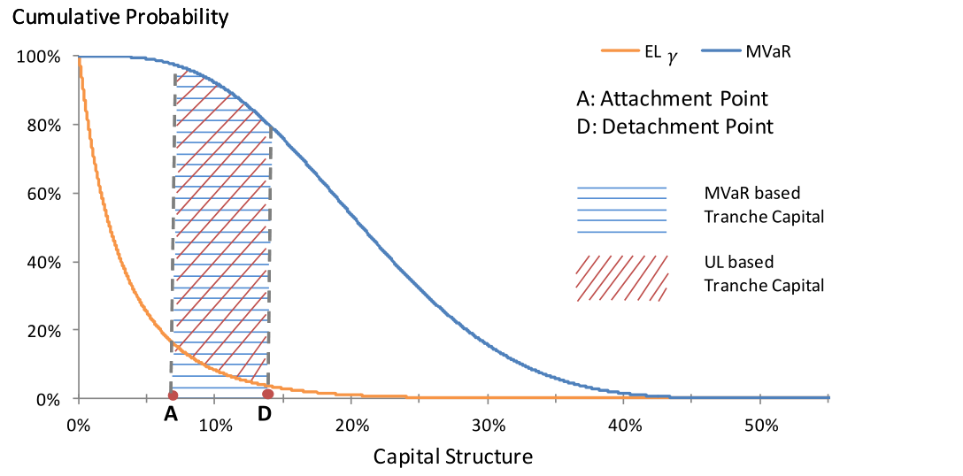
Figure 1 illustrates the above MVaR-based tranche capital. The blue line in the figure equals the MVaR(A, A+ δ) for (infinitesimally) thin tranches (of thickness δ where δ is small) with a particular attachment point, A. Since a thick tranche may be thought of as the sum of a set of thin tranches and MVaR-based capital is additive for individual securities (that collectively make a marginally small contribution to the bank’s overall risk), the MVaR for a thick tranche is just the area under the blue curve between the attachment and detachment point of a given thick tranche.
The red line in Figure 1 shows the ELγ(A, A+ δ) for a thin tranche. Analogously to the argument made above, the Expected Loss with a risk premium for a discretely thick tranche is the area under the red curve, between the attachment and detachment points of that tranche.
The Unexpected Loss of the tranche is defined as the MVaR minus the Expected Loss. The relevant definition of Expected Loss in this case is ELγ. Figure 1 shows Unexpected Loss-based capital for a set of thin tranches as the vertical distance between the Marginal Value-at-Risk (MVaR) curve (shown as blue in the figure) and the Expected Loss with a risk premium (ELγ) curve (shown as red in the figure). UL-based capital is the notion used in IRBA for on-balance sheet loans (prior to securitisation).
Unexpected Losses for thin tranches are not monotonic in seniority. One may observe this from Figure 1 in that the gap between the MVaR and the ELγ curves decreases as the attachment point approaches zero. Regulators express a strong preference for tranche capital that is monotonic in seniority. This can be accommodated within the AFA framework by basing capital on MVaR rather than Unexpected Loss.
Clearly, basing tranche capital on MVaR implies a departure from capital neutrality in that pre- and post-securitisation exposures to the underlying asset pool will no longer be equal. However, if the calibration is performed appropriately, the additional capital introduced by using an MVaR approach is not too onerous and may be regarded as introducing a reasonable amount of conservatism. The subject of this paper is to show how calibration may be performed in a sensible, proportionate manner that is conservative without being excessively onerous.
A second requirement of regulators is a floor on the level of capital. In earlier work, we have argued that the floor should be sensitive either to the level of underlying pool capital or to the pool asset class. We will return to this issue below.
The above model may be employed in a rigorous, bottom-up calculation of securitisation tranche capital given all the underlying parameters. However, the maturity adjustment to capital embodied in the above formula is not directly consistent with the maturity adjustments adopted by the Basel authorities for corporate loans in BCBS (2006).[9]
To ensure a capital neutral outcome, with Unexpected Loss based capital pre- and post-securitisation consistent, in our earlier work on the AFA framework, we advocated replacing PDα,M with the expression:
KPool (8) PDα,M = LGD + PDM
To use equation (8), however, one must have access to an estimate of KPool, under either the IRBA (KIRBA) or the Standardised Approach (KSA). For KPool = KIRBA (excluding the one-year expected loss)[10], one must meet the stringent IRBA informational standards required by Basel regulators. For the Standardised Approach, one can use KPool = KSA.
Nevertheless, to use equation (8), one must also estimate PDM. In Duponcheele et al. (2013b), we proposed to replace[11] equation (8) by equation (9) so that IRBA or Standardised Approach users of the capital formula could employ the model:
KIRBA×CSSFM for IRBA banks LGD (9) PDα,M = { KSA×CSSFM for SA banks LGD
Here, CSSFM is a Capital Surcharge Scaling Factor. Note that the idea here is that the pool Marginal Value at Risk is given by MVaRPool = PDα,M × LGD, so we may approximate[12] the
ELM = ELγ,Pool either with KIRBA × (CSSFM −1) or with KSA × (CSSFM −1) to obtain the inputs necessary to calculate the tranche MVaR(A, D)[13].
The Conservative Monotone Approach or CMA consists of (i) setting PDα,M as in equation (9) and (ii) basing capital on the Marginal VaR capital criterion explained above. The CMA requires as inputs just 8% × RWPool = KIRBA or KSA (depending on whether the bank has access to IRBA or SA inputs), LGD, ρ∗, ρ, and CSSFM.
One should note the following points:
1. Since the CMA takes as one of its primary inputs the risk weight of the securitisation pool, RWPool, the risk hierarchy among asset classes preferred by regulators is respected both before and after securitisation. For example, SME and large corporate BBB/BB-rated loans have risk weights of 75% and 100% respectively, which implies that capital calculated for all securitisation tranches with an SME loan pool will be lower than for a BBB/BB-rated large corporate pool[14].
2. The CMA includes sensitivity to sudden deterioration in the pool since the tranche attachment and detachment points are reduced when pool loans default, provided appropriate definitions are used for A and D. For a discussion on appropriate definitions of A and D, please refer to the Section 7.A of the associated paper Duponcheele et al. (2014b).
Section 3 – regulatory asset classes for securitisations
In this section, we present a set of comprehensive regulatory asset classes for securitisation tranches and parameters for deals representative of each of these classes. In our view, regulatory capital requirements should be designed for broad categories of exposures. Attempts to be over-precise in assigning capital to individual exposures are ill-advised and futile.
We, therefore, think it sensible, in the case of securitisation capital, to base capital requirements on deals representative of particular asset classes. Following this approach will generate capital adequate to cover risks for individual banks with diversified portfolios.
The regulatory asset classes we propose are based on categories and distinctions already employed in the Basel regulatory framework[15]. In the key Basel II document, BCBS (2006), there are 2 frameworks for loans: wholesale and retail. The wholesale framework is subdivided into:
a) Large corporate, sovereign, and bank exposures,
b) SME,
c) Specialised Lending in: c1) Project Finance, c2) Object Finance, c3) Commodities Finance, c4) Income Producing Real Estate, and c5) High Volatility Commercial Real Estate. The retail framework is subdivided into:
a) Residential Mortgage,
b) Qualifying Revolving Retail, and
c) Other Retail.
We base our calibration on these categories, with an additional 3 categories to allow for specific portfolio behaviour, linked to maturity, granularity, or asset quality. The following points are relevant in this regard.
• Most securitisations are granular, but some specific transaction will fall below a specific granularity level. We thus add a category for “Wholesale Non-Granular”.
• Among corporate securitisations, short-maturity trade receivables and trade finance constitute a specific asset class in that such assets behave differently from medium to long term loans.
• Also, the public securitisation market for large corporates is skewed towards the leveraged loan market. To allow for this fact, we split the medium to long term loans between Low Risk weight corporates (less than 125%) and High Risk weight corporates (125% or more).
• Following the crisis, the US authorities introduced two risk-weight categories for residential mortgages (“Category 1” with 50% RW and “Category 2” with 100% RW). In line with this approach, we define a Low Risk Weight residential mortgage category (less than 75%), and a High Risk Weight (75% or more) residential mortgage category.
Tables 2 and 3 present our suggested securitisation asset classes. The definitions of these classes are clearly a matter of judgment but what we propose reflects extensive discussions we have had with securitisation market specialists from many large banks[16].
15 BCBS (2006), paragraphs 215, 216, 217, 218, --, 243. 16 We thank those who gave us views on this topic.
| 2: Proposed | Regulatory | Securitisation Asset Classes | for | the Wholesale | framework, | with description | of real | economy assets | |||||||
|---|---|---|---|---|---|---|---|---|---|---|---|---|---|---|---|
| Proposed | Regulatory | ||||||||||||||
| Meaning | Real life | example | |||||||||||||
| Securitisation | Asset | Class | |||||||||||||
| Trade Receivables, | Trade Finance | (typically | assets | with | 1 to 3 | months | |||||||||
| Granular Short | Term | BCBS128, art 218&230, | and | where the | regulatory | asset | maturity is | ||||||||
| maturity). This is | a relatively large | market in | Europe | and | Asia for | trade | |||||||||
| Bank/Corporate | 1 year or less. | ||||||||||||||
| receivables. Nascent | market for | trade finance | in the | US | and Asia. | ||||||||||
| Granular Low | RW | Medium | |||||||||||||
| Securitisation of | High Grade loans | (typically | risk-weighted | in the | 80%- | ||||||||||
| to Long Term | BCBS128, art 273&230, | and | Low RW | defined as | less than | 125%. | |||||||||
| 100% range). There | is some market | activity in | the | US | and Japan. | ||||||||||
| Bank/Corporate | |||||||||||||||
| Granular High | RW | Medium | Securitisation of | Leveraged Loans | (typically | assets | risk | weighted | at | ||||||
| to Long Term | BCBS128, art 273&230, | and | High RW | defined as | 125% or | more. | 150% or more). | This is a large market | in the | US and | an | important | |||
| Bank/Corporate | market in Europe. | ||||||||||||||
| BCBS128, art 273, corporate | exposures | where the | reported | sales for | Securitisation of | SME loans. This | market is | relevant | for | the European | |||||
| Granular Small- | and | ||||||||||||||
| the consolidated group of | which | the firm is | a part is | less than | €50 | economy (Germany, | Italy, Spain, | UK) but | undeveloped | partly due | to | ||||
| Medium-sized | Entities | ||||||||||||||
| million. | conservative ratings | agency assessments. | US | activity | in | SBA loans. | |||||||||
| BCBS128, art 224, structured | short-term | lending to | finance | ||||||||||||
| Specialised Lending | Securitisation of | Commodities | Finance. This | is a | nascent | market in | |||||||||
| reserves, inventories, or | receivables of | exchange-traded | |||||||||||||
| (Commodities | Finance) | Europe, Russia, | Middle-East Asia | and Latin | America. | ||||||||||
| commodities (e.g. crude | oil, | metals, or | crops). | ||||||||||||
| BCBS128, art 221, large, | complex and | expensive | installations | that | |||||||||||
| Specialised Lending | (Project | might include, for example, | power plants, | chemical | processing | Securitisation of | Project Finance. | ||||||||
| Finance) | plants, mines, transportation | infrastructure, | environment, | and | This is a nascent | market in Europe, | Middle | East, | Latin | America. | |||||
| telecommunications | infrastructure. | ||||||||||||||
| Securitisation of | Transportation | loans. This is | a large | market in the | US | ||||||||||
| Specialised Lending | (Object | ||||||||||||||
| BCBS128, art 223, ships, | aircraft, satellites, | railcars, | and | fleets. | but a small market | in Europe (as | ship finance | is | included | in covered | |||||
| Finance) | |||||||||||||||
| bonds in Europe). | |||||||||||||||
| Specialised Lending | (Income | BCBS128, art 226, office | buildings to let, | retail space, | multifamily | Typically CMBS. | This is a major | market in the | US, | and | an important | ||||
| Producing Real | Estate) | residential buildings, | industrial | or warehouse | space, | and | hotels. | market in UK and | Germany. | ||||||
| Specialised Lending | (High | ||||||||||||||
| BCBS128, art 227, real | estate | assets where | source of | repayment | is | Typically found | in CRE CMBS. | Somewhat | relevant | for | the US and | to | |||
| Volatility Commercial | Real | ||||||||||||||
| substantially uncertain. | a very small degree | the European | market. | ||||||||||||
| Estate) | |||||||||||||||
| Other, such as equity, | capital | venture, private | equity, | etc | Majority of assets | are not first liens | (with very | low | recovery | rates). | |||||
| (BCBS128, art 235 & | 236)… | and/or where | majority | of assets | are | CLOs of Mezzanines | Leveraged | Loans, TRUPS | CDOs. | This is an | |||||
| Other Granular | Wholesale | not first liens (economically | speaking). (This | category | could | also | important market | in the US. | |||||||
| apply to asset pools which | are | not mainly | first liens | or mainly | Typically, CFOs | of Hedge Funds, | Private Equity. | This | is an | ||||||
| senior secured to avoid | LGD | arbitrage). | unrepresentative | and marginal market. | |||||||||||
| Other Non-Granular | |||||||||||||||
| Defined as less than [10] | assets, | excluding | Specialised | Lending. | Marginal private | market, hedging | specific | exposures. | |||||||
| Wholesale |
| 3: Proposed Regulatory | Securitisation | Asset | Classes for the Retail framework, with illustration of | real economy | assets | ||||
|---|---|---|---|---|---|---|---|---|---|
| Proposed regulatory | |||||||||
| Meaning | Real | life example | |||||||
| Securitisation Asset | Class | ||||||||
| Normal Mortgages | (typically | risk weighted | around | ||||||
| Low RW Residential | |||||||||
| BCBS128, | art | 231, | and Low RW defined as less than 75%. | important market for | securitisation | in Europe, | Australia, | ||
| Mortgages | |||||||||
| and Japan. | |||||||||
| High RW Residential | Typically, Subprime | Mortgages. | Dominantly | US | |||||
| BCBS128, | art | 231, | and High RW defined as 75% or more. | ||||||
| Mortgages | presence in Europe | and Australia | |||||||
| BCBS128, | art | 234. | Revolving, unsecured, and uncommitted exposures | Credit Cards. This | is a major | market in the | US and | ||
| Revolving Qualifying | Retail | ||||||||
| to individuals | of less | than 100K EUR. | the UK. | ||||||
| Auto Loans: major | market in | Europe and the | US. | ||||||
| Other Retail | As per the | regulatory | description. | Consumer Loans: | important | market in the | UK and | ||
| Student Loans: major | market | in the US. |
| Table | 4: Choice of | Asset | Class Inputs | and Formulas for the Calibration under | the SA and IRBA | approaches | ||||
|---|---|---|---|---|---|---|---|---|---|---|
| Asset | Maturity Number | of | ||||||||
| correlation17 | ||||||||||
| Proposed | Regulatory | Securitisation Asset Class | Basel | (ρ) | years18 | |||||
| (M) | Exposures | |||||||||
| Granular | Short Term | Bank/Corporate | −e−50×PD1) 12% (1 | + 24% | e−50×PD1 | 1.0 | 50 | |||
| Granular Low | RW | Medium to Long | Term Bank/Corporate | −e−50×PD1) (1 12% | + 24% | e−50×PD1 | 3.0 | 50 | ||
| Granular | High RW | Medium to Long | Term Bank/Corporate | −e−50×PD1) 12% (1 | + 24% | e−50×PD1 | 3.0 | 50 | ||
| −S−5 | ||||||||||
| Granular | Small- and | Medium-sized | Entities 12% (1 | −e−50×PD1) + 24% | e−50×PD1 | −4% × (1 | ) | 2.5 | N/A | |
| 45 | ||||||||||
| Specialised | Lending | (Commodities | Finance) | −e−50×PD1) 12% (1 | + 24% | e−50×PD1 | 5.0 | 20 | ||
| Wholesale | Specialised | Lending | (Project Finance) | −e−50×PD1) (1 12% | + 24% | e−50×PD1 | 5.0 | 20 | ||
| Specialised | Lending | (Object Finance) | −e−50×PD1) 12% (1 | + 24% | e−50×PD1 | 5.0 | 20 | |||
| Specialised | Lending | (Income Producing | Real Estate) | −e−50×PD1) (1 12% | + 30% | e−50×PD1 | 5.0 | 20 | ||
| Specialised | Lending | (High Volatility | Commercial Real Estate) | −e−50×PD1) 12% (1 | + 30% | e−50×PD1 | 5.0 | 20 | ||
| Other Granular | Wholesale | −e−50×PD1) 12% (1 | + 24% | e−50×PD1 | 5.0 | 20 | ||||
| Other | Non-Granular | Wholesale | −e−50×PD1) 12% (1 | + 24% | e−50×PD1 | 5.0 | 5 | |||
| Low RW | Residential | Mortgages | 15% | 4.0 | N/A | |||||
| Retail | High RW | Residential | Mortgages | 15% | 5.0 | N/A | ||||
| Revolving | Qualifying | Retail | 4% | 1.5 | N/A | |||||
| Other Retail | −e−35×PD1) 3% (1 | + 16% | e−35×PD1 | 3.0 | N/A | |||||
| 17 The | only Basel | correlation | formula for | Specialised Lending is given for HVCRE. We | propose to use the | same for | IPRE. For the | other Specialised | Lending subcategories, | |
| proposed | to take the | Basel | corporate | correlation. For SMEs, we chose the value S= | 5. | |||||
| 18 The | calibration | choices | shown in the table | for asset maturity and granularity reflect | the views of | securitisation | risk and structuring | specialists | from multiple banks | and |
| thank | those who | contributed | their views on | these topics. |
| Capital | Capital | ||||||||
|---|---|---|---|---|---|---|---|---|---|
| Expected Loss | |||||||||
| One-Year | Surcharge | Surcharge | |||||||
| Proposed | Regulatory | Choice for19 Choice | for 20 | Granularity- | Probability of | with a risk | Scaling Factor | Scaling Factor | |
| adjusted | premium at | ||||||||
| Securitisation | Asset Class | RWPool | LGDPool | Default | maturity | for Senior for | Non-Senior | ||
| (LGDPool) | Tranches | Tranches | |||||||
| (PD1) | |||||||||
| (ELM) | |||||||||
| (CSSFM) | (CSSFM) | ||||||||
| Granular Short Term | |||||||||
| 100% | 45% | 45.7% | 1.91% | 0.86% | 1.00 | 1.05 | |||
| Bank/Corporate | |||||||||
| Granular Low RW | Medium to Long | ||||||||
| 100% | 45% | 45.7% | 0.88% | 2.42% | 1.05 | 1.18 | |||
| Term Bank/Corporate | |||||||||
| Granular High RW | Medium to | ||||||||
| 150% | 45% | 45.7% | 3.61% | 7.45% | 1.10 | 1.36 | |||
| Long Term Bank/Corporate | |||||||||
| Granular Small- and | Medium-sized | ||||||||
| 75% | 45% | 45.0% | 0.94% | 1.81% | 1.05 | 1.17 | |||
| Entities | |||||||||
| Specialised Lending | (Commodities | ||||||||
| 115% | 25% | 26.8% | 13.06% | 3.26% | 1.00 | 1.18 | |||
| Wholesale | Finance) | ||||||||
| Specialised Lending | (Project | ||||||||
| 70% | 25% | 26.8% | 0.86% | 3.12% | 1.10 | 1.33 | |||
| Finance) | |||||||||
| Specialised Lending | (Object | ||||||||
| 90% | 25% | 26.8% | 2.44% | 6.30% | 1.16 | 1.52 | |||
| Finance) | |||||||||
| Specialised Lending | (Income | ||||||||
| 115% | 45% | 46.8% | 0.33% | 2.95% | 1.06 | 1.19 | |||
| Producing Real Estate) | |||||||||
| Specialised Lending | (High | ||||||||
| 140% | 45% | 46.8% | 0.60% | 4.55% | 1.08 | 1.24 | |||
| Volatility Commercial | Real Estate) | ||||||||
| Other Granular | Wholesale | 150% | 75% | 76.1% | 0.34% | 4.69% | 1.07 | 1.23 | |
| Other Non-Granular | Wholesale | 100% | 45% | 52.8% | 0.44% | 3.44% | 1.08 | 1.26 | |
| Low RW Residential | Mortgages | 35% | 25% | 25.0% | 1.08% | 2.25% | 1.14 | 1.47 | |
| Retail | High RW Residential | Mortgages | 100% | 45% | 45.0% | 2.24% | 9.94% | 1.22 | 1.73 |
| Revolving Qualifying | Retail | 75% | 75% | 75.0% | 3.43% | 4.29% | 1.06 | 1.39 | |
| Other Retail | 75% | 75% | 75.0% | 0.85% | 3.58% | 1.10 | 1.35 | ||
| 19 The | risk weights were | chosen based on Standardised | Approach values, | and in the | case of Specialised | Lending, based on | the Slotting Criteria | Approach values. | |
| 20 The | LGDs were chosen | based on the IRB-Foundation | Approach for | corporates, as | well as a conservative | judgement in | other categories. The | level of conservatism | can |
| assessed | by comparing IRBA | LGDs provided in | Appendix 3, Table A3.1. |
| 1-Year | M-Year | ||||||||||||
|---|---|---|---|---|---|---|---|---|---|---|---|---|---|
| BCBS | |||||||||||||
| Intra-sector | Conditional | Conditional | Granularity- | ||||||||||
| Systemic | |||||||||||||
| Proposed | Regulatory | Securitisation Asset Class | correlation21 | Pool | Pool | adjusted | |||||||
| Correlation | |||||||||||||
| (ρs,s) | (ρ)22 | Correlation | Correlation | ∗) (ρM | |||||||||
| (ρ∗) | ∗) | ||||||||||||
| (ρM | |||||||||||||
| Granular | Short Term | Bank/Corporate | 75.82% | 16.62% | 6.35% | 6.35% | 8.22% | ||||||
| Granular Low | RW | Medium to Long | Term Bank/Corporate | 75.82% | 19.73% | 7.84% | 20.82% | 22.40% | |||||
| Granular | High RW | Medium to Long | Term Bank/Corporate | 75.82% | 13.97% | 5.18% | 14.44% | 16.15% | |||||
| Granular | Small- and | Medium-sized | Entities | 76.27% | 15.50% | 5.71% | 15.07% | 15.07% | |||||
| Specialised | Lending | (Commodities | Finance) | 61.45% | 12.02% | 8.57% | 8.57% | 13.14% | |||||
| Wholesale | Specialised | Lending | (Project Finance) | 61.45% | 19.81% | 15.48% | 29.41% | 32.94% | |||||
| Specialised | Lending | (Object Finance) | 61.45% | 15.54% | 11.54% | 22.89% | 26.74% | ||||||
| Specialised | Lending | (Income Producing | Real Estate) | 74.65% | 27.26% | 12.72% | 32.85% | 36.20% | |||||
| Specialised | Lending | (High Volatility | Commercial Real Estate) | 74.65% | 25.33% | 11.54% | 30.44% | 33.92% | |||||
| Other Granular | Wholesale | 75.82% | 22.12% | 9.06% | 25.89% | 29.59% | |||||||
| Other | Non-Granular | Wholesale | 75.82% | 21.63% | 8.79% | 25.27% | 40.22% | ||||||
| Low RW | Residential | Mortgages | 75.05% | 10.00% | 3.69% | 11.10% | 11.10% | ||||||
| Retail | High RW | Residential | Mortgages | 75.05% | 10.00% | 3.69% | 11.56% | 11.56% | |||||
| Revolving | Qualifying | Retail | 69.96% | 4.00% | 1.79% | 3.13% | 3.13% | ||||||
| Other Retail | 78.34% | 12.65% | 4.01% | 12.48% | 12.48% | ||||||||
| 21 Source: | Risk Control | Limited: | those values | are used for both IRBA | and | SA | calibration | ||||||
| 22 | |||||||||||||
| Calculated using | PD1 in | Table 5. The one | exception in our use of | BCBS | systemic | correlations is | for residential | mortgages. In Basel | II, the systemic | correlation for | residential | ||
| mortgages | was set | at the | value | of 15% not | because this was thought | to | be a | plausible estimate of | the true asset | correlation for | this asset class, | but instead to take | account |
| (in an | approximate | way) of | the | typically long | maturities of residential | mortgages | (The issue of | potential double | counting the maturity | effect was | mentioned explicitly | in Basel | |
| (2012)). | We, therefore, | choose | to use a | conservative value for | residential | mortgages of 10%. |
| Proposed | Regulatory | Securitisation Asset Class | 100% | 90% | 80% | 70% | 60% | 50% | 40% | 30% | 20% | 10% | 0% | |
|---|---|---|---|---|---|---|---|---|---|---|---|---|---|---|
| Granular | Short Term | Bank/Corporate | 1.00 | 1.01 | 1.02 | 1.03 | 1.04 | 1.05 | 1.06 | 1.08 | 1.09 | 1.10 | 1.11 | |
| Granular Low | RW | Medium to Long | Term Bank/Corporate | 1.05 | 1.08 | 1.10 | 1.13 | 1.15 | 1.18 | 1.20 | 1.23 | 1.25 | 1.28 | 1.30 |
| Granular | High RW | Medium to Long | Term Bank/Corporate | 1.10 | 1.15 | 1.20 | 1.25 | 1.31 | 1.36 | 1.41 | 1.46 | 1.52 | 1.57 | 1.62 |
| Granular | Small- and | Medium-sized | Entities | 1.05 | 1.07 | 1.10 | 1.12 | 1.15 | 1.17 | 1.20 | 1.23 | 1.25 | 1.28 | 1.30 |
| Specialised | Lending | (Commodities | Finance) | 1.00 | 1.04 | 1.07 | 1.11 | 1.14 | 1.18 | 1.21 | 1.25 | 1.28 | 1.32 | 1.35 |
| Specialised | Lending | (Project Finance) | 1.10 | 1.15 | 1.19 | 1.24 | 1.29 | 1.33 | 1.38 | 1.42 | 1.47 | 1.51 | 1.56 | |
| Specialised | Lending | (Object Finance) | 1.16 | 1.23 | 1.30 | 1.37 | 1.44 | 1.52 | 1.59 | 1.66 | 1.73 | 1.80 | 1.88 | |
| Specialised | Lending | (Income Producing | Real Estate) | 1.06 | 1.09 | 1.11 | 1.14 | 1.16 | 1.19 | 1.22 | 1.24 | 1.27 | 1.29 | 1.32 |
| Specialised | Lending | (High Volatility | Commercial Real Estate) | 1.08 | 1.11 | 1.14 | 1.18 | 1.21 | 1.24 | 1.27 | 1.31 | 1.34 | 1.37 | 1.41 |
| Other Granular | Wholesale | 1.07 | 1.11 | 1.14 | 1.17 | 1.20 | 1.23 | 1.26 | 1.30 | 1.33 | 1.36 | 1.39 | ||
| Other | Non-Granular | Wholesale | 1.08 | 1.12 | 1.15 | 1.19 | 1.22 | 1.26 | 1.29 | 1.32 | 1.36 | 1.39 | 1.43 | |
| Low RW | Residential | Mortgages | 1.14 | 1.21 | 1.27 | 1.34 | 1.41 | 1.47 | 1.54 | 1.60 | 1.67 | 1.74 | 1.80 | |
| High RW | Residential | Mortgages | 1.22 | 1.33 | 1.43 | 1.53 | 1.63 | 1.73 | 1.83 | 1.94 | 2.04 | 2.14 | 2.24 | |
| Revolving | Qualifying | Retail | 1.06 | 1.12 | 1.19 | 1.25 | 1.32 | 1.39 | 1.45 | 1.52 | 1.58 | 1.65 | 1.71 | |
| Other Retail | 1.10 | 1.15 | 1.20 | 1.25 | 1.30 | 1.35 | 1.40 | 1.45 | 1.50 | 1.55 | 1.60 |
Section 4 – calibration of the cma
Calibrating the Capital Surcharge Scaling Factor CSSFM
The Capital Surplus Scaling Factor CSSFM depends on (i) the expected loss (inclusive of a risk premium after the first year), (ii) the pool capital, and (iii) the level of future margin income recognition.
To infer an appropriate Expected Loss (inclusive of a risk premium after the first year), one may use the equation: M−1 (10) ELM = ELγ,Pool = LGDPool × N (N−1(pdM) + √M × γ) where pdM is the M-year default probability, and γ is the risk premium.
We infer the M-year default probability, pdM from the one-year default probability PD[1] using an approach suggested in Basel Working Paper 23 (BCBS, 2013b, pg. 8) using the equation:
(11) pdM = 1+exp(−ln( PD1 1−PD1) − (5−0.15×ln (1−PD1 ))(M0.2−1))
We follow BCBS (2013a, pg. 19) in using the following approach to specify a risk premium:
(12) γ= λ∙√ρ
As in BCBS (2013a), we use a λ value of 0.4.
For senior tranches, it appears excessively conservative to give no recognition to Future Margin Income (FMI) in calculating capital. In the pre-securitisation IRBA capital framework, FMI is recognised by subtracting the one-year expected loss EL[1] = PD[1] × LGD (see equation (22) from the one-year Marginal Value at Risk before the resulting UL is scaled up for maturity).
In the securitisation framework (to ensure that tranche capital is monotonic in seniority), regulators have based capital on Marginal Value-at-Risk, inclusive of Expected Losses. For senior tranches only, the Basel proposal (BCBS (2013c)) proposes to recognise 80% of the FMI beyond the one-year horizon.
A simple way of allowing for FMI (and one which permits us to retain the use of Capital Surcharge Scaling Factors) is to consider FMI at the pool level[23] and to treat it as resembling a reserve account reducing the net value of the required pool capital. One may then use the tranche MVaR function set out in Section 2 to distribute the net capital across tranches.
For senior tranches, Future Margin Income may be recognised as covering 100% of Expected Losses for period 1 and 80% of Expected Losses after period 1 (FMISenior = EL[1] + 0.8 × (ELM −EL[1])). Then, total pool Expected Losses relevant for senior tranches would be (ELM −FMISenior). In this case, one may define the Capital Surcharge Scaling Factor to be:
ELM−FMISenior 0.2×ELM−0.2×EL1 = 1 + (13) CSSFM = 1 + KPool KPool
For non-senior tranches, one may conservatively consider that the FMI makes a smaller impact in reducing the net pool capital. If we suppose that FMI contributes 50% of the contribution we allowed for in the case of senior tranches, namely 0.5 × FMISenior, then total pool Expected Losses relevant for non-senior tranches would be:
(14) ELM −0.5 × (EL[1] + 0.8 × (ELM −EL[1])) = 0.6 × ELM −0.1 × EL[1]
So the Capital Surcharge Scaling Factor, CSSFM, for non-senior tranches should be:
0.6×ELM−0.1×EL1 (15) CSSFM = 1 + KPool
Table 7 provides a sensitivity analysis, under the Standardised Approach calibration by showing what the consequences are on the capital surcharge scaling factor for non-senior tranches of assuming a percentage of FMISenior other than 50%. The ratio of 50% implies a capital surcharge of 73% for High RW residential mortgages. If the ratio is 0%, the calibration shows a capital surcharge of up to 124% for non-senior tranches of High RW residential mortgages.
∗ Calibrating the Conditional Pool Correlation, ρM
The maturity effect, M, on the conditional pool correlation is given in Duponcheele et al. (2013c), by the following equation, with the asset maturity, M, the systemic correlation, ρ, and the pool correlation, ρPool:
M×ρPool−ρ ∗ = (16) ρM M−ρ
The pool correlation ρPool is given by Duponcheele et al. (2013a) as:
(17) ρPool = ρ+ (1 −ρ) × ρ∗
Here, ρ∗ is the one-year asset class-specific conditional pool correlation, defined for each asset class.
The one-year asset-class specific conditional pool correlation is itself determined by the formula:
ρ×(1−ρs,s) ρ∗ = (18) (1−ρ)×ρs,s
Here, ρs,s is calculated by the methodology exposited in Duponcheele et al. (2013a) provided by Risk Control Limited, and provided in Table 6, column 1. When combined with the maturity M and the Basel correlation (without maturity double counting) (itself dependent on PD[1]), using equations (16), (17) and (18), one obtains the values that appear in Table 6, column 2, for the Systemic Correlation, ρ, and Table 6, column 3, for the One-Year Conditional Pool Correlation, ρ∗, and Table 6, column 4, for the ∗ . Conditional Pool Correlation, ρM
Calibrating the effect of granularity ( N)
The last adjustment concerns granularity. The granularity is the inverse of N, defined as the number of effective exposures in the regulatory sense (for example, as in BCBS (2006)).
When appropriate, granularity can be taken into account by replacing the inputs in the CMA formula in equations (2) and (4): (1−1 N)) (19) LGDPool → LGDPool (LGDPool
∗ + ∗ )) (20) ρM∗ → (ρM N (1 −ρM
For N> 100, granularity has no material impact on the distribution across tranches of the pool Marginal Value at Risk. Equations (19) and (20) would apply only to the wholesale framework as it can be fairly assumed that retail securitisations are highly granular in the banking system.
As shown in Duponcheele et al. (2013d), granularity is a significant risk driver only when the effective number of assets is below 100, in which case one may adjust the correlations. When the effective number is below 10, it is appropriate also to adjust the loss-given default assumptions.
For calibration purpose, the choice for the number of effective exposures for the pool, N, is given in Table 4, column 3. The choice reflects the views of securitisation risk and structuring specialists from multiple banks and has been made with a view to calibrating conservatively the different asset classes. N was set at no more than 50 for Corporate securitisation and no more than 20 for Specialised Lending. Wholesale SMEs and Retail categories were deemed granular. For the rare wholesale securitisations (other than Specialised Lending) where N< 10, the calibration was done with N= 5 in a special category called “Other Non-granular Wholesale”.
Data on the effects of granularity on our calibration of the Granularity-adjusted LGDPool may be found in Table 5, column 3. Those values were used for Table 1, column 1. However, we could simplify the framework further to have a granularity adjusted LGDPool only for the securitisation regulatory asset class “Other Non-granular Wholesale”. For all other categories, without losing much risk sensitivity, instead of using the granularity adjusted LGDPool from Table 5, column 3, we could simply use the nonadjusted values as shown in Table 5, column 2.
∗ may be found in Data on the effects of granularity on our calibration on the Granularity-adjusted ρM Table 6, column 5. Those values were taken for Table 1, column 2.
Section 5 – standardised approach calibration
In this section, we show how to deduce CMA inputs for a comprehensive set of securitisation regulatory asset classes under the Standardised Approach. The steps involve: (i) choosing primitive inputs for deals representative of each asset class, (ii) calculating the Capital Surcharge Scaling Factor, CSSFM, (iii) ∗ , and (iv) calculating granularity adjustments. inferring the Conditional Pool Correlation, ρM
Calibrating the primitive inputs for each asset class
Under the SA calibration, the RWPool, LGDPool are asset class-specific calibration choices and the PD[1] is reverse engineered from the capital level. Table 5 shows the input values we would suggest.
The choices for the pool maturity, M (minimum 1 year, maximum 5 year) are given in Table 4, column
2. These choices reflect the views of securitisation risk and structuring specialists from multiple banks. The choice was not driven by specific transactions, but rather by an estimate of the average maturity in the banking system as a whole.
The choices for BCBS (2006) systemic correlation formula are given in Table 4, column 1. This is based on the framework itself for all categories bar for Specialised Lending. Since the framework provides a systemic correlation only for the High Volatility Commercial Real Estate category, the same correlation was chosen for the Income Producing Real Estate category. For the other specialised lending a corporate correlation was chosen.
Inferring PD[1]
To evaluate this, we calculate (21) KPool = RWPool × 8%
and then infer PD[1] by inverting the following equation:
N−1(PD1)+N−1(99.9%)×√ρ (22) KPool = 1.06 × (LGD× N ( √1−ρ ) −PD[1] × LGD) × MatAdj(M)
Note that, in the wholesale framework, the maturity adjustment factor in equation (22) takes the form:
1+(M−2.5)×b MatAdj(M) = 1−1.5×b and b= (0.11852 −0.05478 × ln (PD[1]))[2] (23)
whereas, in the retail framework, MatAdj(M) = 1.0. (The non-linear nature of the dependence of IRBA capital on the PDs of the underlying pool assets implies that a conservative value for PD[1] may be obtained by inverting the above equation.)
This yields the values of PD[1] in Table 5, column 4. Given values of PD[1] for each regulatory asset class, we infer appropriate, asset-class-specific values for the Capital Surplus Scaling Factor, CSSFM, by following the steps described in Section 4.
Using equations (10), (11), and (12) with λ= 0.4, one may infer the Expected Losses ELM shown in Table 5, column 5. From this Expected Loss, and after adjustment for FMI, and the known value of KPool, using equations (13) and (15) we infer the CSSFM values given in Table 5, column 6 and column 7, for senior and non-senior tranches respectively. Those values are also reported in Table 1, column 3 and 4.
Summary
Table 8 summarises our proposals for regulatory inputs to the CMA for the different asset classes, both for senior and non-senior tranches.
One may make the following remarks on the capital surcharge and conditional pool correlation proposed in the table.
• When comparing the Low RW and the High RW calibration for corporates and for residential mortgages, the capital surcharge increases with asset risk. Examples: for senior tranches, 5% vs. 10% for corporates and 14% vs. 22% for residential mortgages; for non-senior tranches, 18% vs. 36% for corporates and 47% vs. 73% for residential mortgages.
• Beyond the one-year horizon, the capital surcharge increases with structural risk when one compares senior tranches vs. non-senior tranches. Example: for Low RW residential mortgages, that is 14% for senior tranches vs. 47% for non-senior tranches.
• The combination of higher asset risk and higher structural risk deepens the widening of the capital surcharge. The capital surcharge for senior tranches of Low RW residential mortgages is 14% vs. 73% for non-senior tranches of High RW residential mortgages.
• The highest capital surcharge among the asset classes is for the High RW residential mortgages (73% for non-senior tranches), which also corresponds to the lessons from the crisis.
• When comparing the short maturity and long maturity asset classes, the conditional pool correlation increases with asset maturity. An example is the 8% value for short term corporates (trade receivables) versus the 22% value for medium to long term corporates.
Granular Low RW Medium to Long Term 46% 22% 1.05 1.18 Bank/Corporate Granular High RW Medium to Long Term 46% 16% 1.10 1.36 Bank/Corporate Granular Small- and Medium-sized Entities 45% 15% 1.05 1.17 Specialised Lending (Commodities Finance) 27% 13% 1.00 1.18 Specialised Lending (Project Finance) 27% 33% 1.10 1.33 Specialised Lending (Object Finance) 27% 27% 1.16 1.52 Specialised Lending (Income Producing Real 47% 36% 1.06 1.19 Estate) Specialised Lending (High Volatility 47% 34% 1.08 1.24 Commercial Real Estate) Other Granular Wholesale 76% 30% 1.07 1.23 Other Non-Granular Wholesale 53% 40% 1.08 1.26 Low RW Residential Mortgages 25% 11% 1.14 1.47 High RW Residential Mortgages 45% 12% 1.22 1.73 Retail Revolving Qualifying Retail 75% 3% 1.06 1.39 Other Retail 75% 12% 1.10 1.35
| Securitisation Regulatory Asset Class | LGD | CSSFM ∗ ρM Senior | |
|---|---|---|---|
| h Granular Short Term Bank/Corporate | 46% | 8% | 1.00 |
Section 6 – irba calibration
Under the IRBA approach, the CMA calibration follows the same four steps described in Section 5 for the SA calibration with the following differences.
Under the IRBA calibration, the PD[1] and LGDPool are actual IRBA inputs, and we calculate the KPool (and RWPool) with the IRBA capital requirement formula. This KPool differs from KIRB (BCBS (2006)) and BCBS (2013c) as EL[1] is not added back as is the case in KIRB. We will refer to it as KIRBA.
For the purpose of calibration, we have used the same pool maturity and granularity values as the ones provided in Table 3, column 2.
With KPool known, using the same assumptions as for the risk premium parameter (γ= 0.4 × √ρ) and for FMI recognition, one can derive the CSSFM under IRBA for senior tranches using equation (13) and for non-senior tranches using equation (15).
0.2×ELM−0.2×EL1 (24) CSSFM = 1 + KPool
0.6×ELM−0.1×EL1 (25) CSSFM = 1 + KPool
ELM EL1 By setting f(PD[1], ρ, λ, M) = KPool and g(PD[1], ρ) = KPool, we can write equations (13) and (15) as:
(26) CSSFM = 1 + α[1] × f(PD[1], ρ, λ, M) −α[2] × g(PD[1], ρ)
One may deduce from equation (26) that the capital surcharge scaling factor CSSFM in IRBA mode is not sensitive to LGDPool, as this variable is both in the numerator and denominator of the ratio for f( ) and g( ).
One may also deduce from equation (26), that the capital surcharge scaling factor CSSFM in IRBA increases when λ (which drives the risk premium) increases.
The other sensitivities to PD[1], ρ and M are more complex to assess, but the results are the following: CSSFM increases, ceteris paribus,
• when the pool maturity increases and this positive sensitivity is higher for retail pools than for wholesale pools given the maturity adjustment effect in the KPool for wholesale pools[24];
• when the Basel systemic correlation ρ decreases;
• when PD[1] increases and this positive sensitivity is higher for non-senior tranches than for senior tranches. In the CMA model, the low risk assets will attract less capital surcharge than the high risk assets. This outcome is prudent. (In the BCBS (2013c) proposals, for the IRBA SSFA, the parameter C is negative, leading to more capital surcharge for low risk assets and less capital surcharge for high risk assets).
To calibrate PD[1] under the IRBA approach, we have used for each asset classes IRBA-approved PD[1] estimates provided by several banks participating in the AFA Quant Group. These banks have also provided IRBA-approved LGDPool for the relevant asset classes. For confidentiality reasons, we do not disclose here the IRBA-approved PD[1] and LGDPool for individual banks or individual transactions. However, we disclose the average RWPool and LGDPool per asset classes and inferred CSSFM estimates (see Table 9).
| IRBA | IRBA | |||||
|---|---|---|---|---|---|---|
| CSSFM | ||||||
| Securitisation | Regulatory Asset Class | RW | LGD | ∗ | ||
| ρM | Senior | Non-Senior | ||||
| (Input) | (Input) | |||||
| Granular Short Term | Bank/Corporate | 86% | 37% | 8% | 1.00 | 1.06 |
| Granular Low RW | Medium to Long Term | |||||
| 76% | 37% | 23% | 1.05 | 1.17 | ||
| Bank/Corporate | ||||||
| Granular High RW | Medium to Long Term | |||||
| 184% | 46% | 14% | 1.12 | 1.47 | ||
| Bank/Corporate | ||||||
| Granular Small- and | Medium-sized Entities | 85% | 41% | 12% | 1.07 | 1.26 |
| Specialised Lending | (Commodities | |||||
| 92% | 32% | 14% | 1.00 | 1.10 | ||
| Finance) | ||||||
| Specialised Lending | (Project Finance) | 23% | 11% | 35% | 1.08 | 1.26 |
| Specialised Lending | (Object Finance) | 38% | 11% | 25% | 1.17 | 1.57 |
| Specialised Lending | (Income Producing | |||||
| 84% | 27% | 32% | 1.09 | 1.27 | ||
| Real Estate) | ||||||
| Specialised Lending | (High Volatility | |||||
| 203% | 52% | 23% | 1.16 | 1.53 | ||
| Commercial Real | Estate) | |||||
| Other Granular | Wholesale | 130% | 52% | 28% | 1.10 | 1.30 |
| Other Non-Granular | Wholesale | 88% | 38% | 38% | 1.11 | 1.35 |
| Low RW Residential | Mortgages | 12% | 22% | 11% | 1.12 | 1.39 |
| High RW Residential | Mortgages | 124% | 43% | 12% | 1.23 | 1.77 |
| Revolving Qualifying | Retail | 41% | 45% | 3% | 1.06 | 1.37 |
| Other Retail | 61% | 42% | 8% | 1.17 | 1.63 |
Conclusion
This paper sets out a variant of the Arbitrage Free Approach (AFA) to securitisation developed by Duponcheele et al. (2013a, b, c, d). This variant, the Conservative Monotone Approach (CMA), adopts a Marginal VaR-criterion for capital rather than the Unexpected Loss criterion employed by the Basel II on-balance sheet loan capital charges. This ensures that capital is monotonically decreasing in seniority, a characteristic of a securitisation framework preferred by regulators. A floor to capital is also imposed.
Having exposited the model, we show how to calibrate the CMA for a set of representative exposures corresponding to individual regulatory asset classes. The approach we take to calibration is informationally economical. Given a standardised pool capital input, KSA, any investor bank may ∗ in Table 1. calculate the capital charges using the parameters LGDP, CSSFM, and ρM
Banks with access to IRBA information on the underlying pool (PD[1], LGD, ρ, and M) may first use those values to calculate the capital surcharge scaling factor CSSFM and conditional pool correlation ∗ , before calculating the capital charges of a tranche using the IRBA pool capital requirement prior to ρM securitisation, KIRBA and IRBA LGDIRBA.
Alternatively, without losing much risk sensitivity, banks with access to IRBA information could ∗ , and use only the pool capital simply use the same coefficients as in Table 1 for CSSFM and ρM requirement prior to securitisation, KIRBA and LGDIRBA.
The asset-class-based calibration has the major advantage that one may calculate capital in a risksensitive way. Based on information available to investors, our approach allows not just to calculate (i) total pool capital but also (ii) the distribution of pool capital to junior and senior tranches, and (iii) the capital surplus (the ratio of pre- to post securitisation capital) to vary for low and high risk securitisations.
The current Basel proposal (see BCBS (2013c)) offers much more limited risk sensitivity unless the bank calculating the capital has access to IRBA information on pool assets, which, realistically, only applies for originators.
References
Basel Committee on Banking Supervision (2001) “Treatment of Asset Securitisation,” Bank for International Settlements, BCBS Working Paper 10, October.
Basel Committee on Banking Supervision (2002) “Second Working Paper on Securitisation,” Bank for International Settlements, BCBS Working Paper 11, October.
Basel Committee on Banking Supervision (2006) “Basel II: International Convergence of Capital Measurement and Capital Standards: A Revised Framework - Comprehensive Version,” Bank for International Settlements, BCBS No.128, June.
Basel Committee on Banking Supervision (2009) “Enhancements to the Basel II framework,” Bank for International Settlements, BCBS No.157, July.
Basel Committee on Banking Supervision (2012) “Revisions to the Basel Securitisation Framework,” Bank for International Settlements, BCBS No.236, December.
Basel Committee on Banking Supervision (2013a) “Foundations of the Proposed Modified Supervisory Formula Approach,” Bank for International Settlements, Working Paper 22, January.
Basel Committee on Banking Supervision (2013b) “The Proposed Revised Ratings-Based Approach,” Bank for International Settlements, Working Paper 23, January.
Basel Committee on Banking Supervision (2013c) “Revisions to the securitisation framework,” Consultative Document, Bank for International Settlements, December.
Basel Committee on Banking Supervision (2013d) “The regulatory framework: balancing risk sensitivity, simplicity and comparability,” Discussion Paper, Bank for International Settlements, July.
Duponcheele, Georges, William Perraudin and Daniel Totouom-Tangho (2013a) “A Principles-Based Approach to Regulatory Capital for Securitisations,” BNP-Paribas mimeo, April. http://www.riskcontrollimited.com/public/Regulatory_capital_for_securitisations.pdf
Duponcheele, Georges, William Perraudin and Daniel Totouom-Tangho (2013b) “The Simplified Arbitrage-Free Approach: Calculating Securitisation Capital based on Risk Weights Alone,” BNP- Paribas mimeo, July. http://www.riskcontrollimited.com/public/Simplified_AFA_revised.pdf
Duponcheele, Georges, William Perraudin and Daniel Totouom-Tangho (2013c) “Maturity Effects in Securitisation Capital: Total Capital Levels and Dispersion Across Tranches,” BNP-Paribas mimeo, September. http://www.riskcontrollimited.com/public/Maturity_Effects_in_Securitisation_Capital.pdf
Duponcheele, Georges, William Perraudin, Alastair Pickett and Daniel Totouom-Tangho (2013d) “Granularity, Heterogeneity and Securitisation Capital,” BNP-Paribas mimeo, September. http://www.riskcontrollimited.com/public/Granularity_Heterogeneity_and_Securitisation_Capital.pdf
Duponcheele, Georges, William Perraudin and Daniel Totouom-Tangho (2014a) “Reducing the Reliance of Securitisation Capital on Agency Ratings,” BNP-Paribas mimeo, February. http://www.riskcontrollimited.com/public/Reducing_the_Reliance.pdf
Duponcheele, Georges, William Perraudin and Daniel Totouom-Tangho (2014b) “Calibration of the Simplified Supervisory Formula Approach,” BNP-Paribas mimeo, March. http://www.riskcontrollimited.com/public/Calibration_of_SSFA.pdf
Pykhtin, Michael and Ashish Dev (2002) “Credit Risk in Asset Securitisations: Analytical Model,” Risk, 15(5), S16-S20, May.
Appendix 1 implementation of the mvar function
∗ ) (A1.1) KCMA(l, u) = MVaRTrancℎe(l, u, RWP, LGDP, CSSFM, ρM
For a performing pool P, there are 7 key inputs to the MVaR function of the CMA: 3 inputs for the tranche: l and u and whether a tranche is senior or not, ∗ 4 regulatory risk drivers for the pool: RWP, LGDP, CSSFM, ρM
1. Lower boundary of the tranche: l
2. Upper boundary of the tranche: u
3. Pool risk weight: RWP
4. Asset loss given default: LGDP
5. Capital surcharge scaling factor: CSSFM, depending on seniority of the tranche ∗ .
6. Conditional pool correlation: ρM
With those inputs:
(A1.2) MVaRTrancℎe = 12.5 × SPDTrancℎe(l) × SLGDTrancℎe(l, u)
Where SPDTrancℎe(l) is the tranche probability of default conditional to a stress and SLGDTrancℎe(l, u) is the tranche loss given default conditional to a stress.
CSSFM By defining the conditional pool probability of default SPDP = RWP ∙8% ∙ LGDP , we can write the two functions:
x ∗ N−1(SPDP) − N−1( LGDP)×√1−ρM ) (A1.3) SPDTrancℎe(x) = N ( ∗ √ρM
and SPDTrancℎe(u) ( BV(l)−BV(u) LGDP SPDTrancℎe(l)×u)−l + (A1.4) SLGDTrancℎe(l, u) = (u−l) (u−l) × (SPDTrancℎe(l))
∗ ) with N[2](a, b, r) being the bivariate where BV(x) = N[2](N−1(SPDP), N−1(SPDTrancℎe(x)), √ρM ) function is easily implementable in Excel cumulative standard normal distribution function. The N[2]( using VBA.
Special cases for equation (A1.3): If (x≥LGDP) then SPDTrancℎe(x) = 0% If (x= 0) then SPDTrancℎe(0) = 100%
Special cases for equation (A1.4): If (l≥LGDP) then SLGDTℎickTrancℎe(l, u) = 0% If (x≥LGDP) then BV(x) = 0% If (x= 0) then BV(0) = SPDP.
Appendix 2 practical implementation of the cma
In this section, we discuss in detail the calculation of the various inputs to the CMA.
Calculating KP and KW for the CMA
One may determine the portfolio capital requirement KPool to be used as an input into the regulatory securitisation formula.
We start by determining EADPool, the Pool Exposure at Default, as being the sum of all EADasset, the Exposure at Default of each asset in the pool:
for eacℎ (A2.1) EADPool = ∑ EADasset asset
We determine the Pool Delinquent Exposure at Default, EADW, as being the sum of all EADdelinquent asset, the Exposure at Default of each delinquent asset in the pool:
(A2.2) for eacℎ EADW = ∑ EADdelinquent asset delinquent asset
The delinquency ratio W is given as the ratio of the Pool Delinquent Exposure at Default to the Pool Exposure at Default:
EADW W= (A2.3) EADPool
The Pool Performing Exposure at Default, EADP, is defined as the sum of all EADperforming asset, the Exposure at Default of each performing asset (defined as not being a delinquent asset) in the pool:
(A2.4) for eacℎ EADP = ∑ EADperforming asset performing asset
Since the following relationship holds:
(A2.5) EADPool = EADP + EADW
It is the case that:
(A2.6) EADP = (1 −W) × EADPool
One can calculate the Pool Risk Weighted Assets, RWAPool, by adding the Pool Delinquent Risk Weighted Assets, RWAW, and the Pool Performing Risk Weighted Assets, RWAP:
(A2.7) RWAPool = RWAP + RWAW
We determine the Pool Delinquent Risk Weighted Assets, RWAW, for all the delinquent assets in the pool as being the sum of all RWAdelinquent asset, the Risk Weighted Asset of each delinquent asset in the pool:
(A2.8) for eacℎ RWAW = ∑ RWAdelinquent asset delinquent asset
We determine the Pool Delinquent Capital Requirement KW (as percentage) as the ratio of the Pool Delinquent Risk Weighted Assets, RWAW, to the Pool Delinquent Exposure at Default, EADW, divided by 12.5:
RWAW (A2.9) KW = EADW×12.5
We determine the Pool Performing Risk Weighted Assets, RWAP, for all the performing assets in the pool (defined as being non-delinquent assets) as being the sum of all RWAperforming asset, the Risk Weighted Asset of each performing asset in the pool:
(A2.10) for eacℎ RWAP = ∑ RWAperforming asset performing asset
We determine the Pool Performing Capital Requirement KP (as percentage) as the ratio of the Pool Performing Risk Weighted Assets, RWAP, to the Pool Performing Exposure at Default, EADP, divided by 12.5:
RWAP (A2.11) KP = EADP×12.5
Since we can develop the relationship from equation (A2.7):
RWAPool = RWAP + RWAW
(A2.12) KPool × EADPool × 12.5 = KP × EADP × 12.5 + KW × EADW × 12.5
EADP EADW (A2.13) KPool = EADPool × KP + EADPool × KW
We have thus the relationship for the Pool Capital Requirement KPool expressed as a percentage:
(A2.14) KPool = (1 −W) × KP + W× KW
Determination of KP and KW in IRB-A/IRB-F:
• For the delinquent asset, we have:
The Exposure representing Expected Loss, EELdelinquent asset, for a delinquent asset is given by the product of the Loss Given Default LGDdelinquent asset and the Exposure at Default for the relevant delinquent asset:
(A2.15) EELdelinquent asset = LGDdelinquent asset × EADdelinquent asset
For a delinquent asset with a given Impairement, the Exposure representing loss in Excess of expected loss, EXSdelinquent asset, is given by the greater of zero and the difference between the Impairment and the Loss Given Default, times the Exposure at Default:
EXSdelinquent asset = max(Impairement−LGDdelinquent asset, 0) × EADdelinquent asset (A2.16)
The Risk Weighted Asset, RWAdelinquent asset, of a delinquent asset will be the sum of the Exposure representing Expected Loss, EELdelinquent asset, and the Exposure in Excess of Expected Loss, EXSdelinquent asset, for that delinquent asset, times 12.5:
(A2.17) RWAdelinquent asset = (EELdelinquent asset + EXSdelinquent asset) × 12.5
Since we have the relationship (A2.8) and (A2.9), we can obtain KW in equation (A2.14):
• For the performing (i.e., non-delinquent) assets, we have:
The capital requirement K with the formula using systemic correlation (AVC), one-year probability of default (PD) and loss-given default (LGD), and when relevant asset maturity (M), (or directly K= RW× 8% with the slotting criteria approach).
RWAperforming asset = Kperforming asset × 1.06 × 12.5 × EADperforming asset (A2.18)
Since we have the relationship (A2.10) and (A2.11), we can obtain KP in equation (A2.14).
We can thus obtain in IRB-A/IRB-F the capital requirement of the pool, as in equation (A2.14):
KPool = (1 −W) × KP + W× KW
Determination of KP and KW in Standardised Approach:
• For the delinquent asset, we have (according to BCBS (2013c)):
(A2.19) KW = 0.5
which implies that RWAW = 625% × EADW
• For the performing asset, we have (according to BCBS (2013c)):
(A2.20) KP = KSA
We can thus obtain in SA, the capital requirement of the pool, as in equation (A2.14)
KPool = (1 −W) × KP + W× KW
or when developed:
(A2.21) KPool = (1 −W) × KSA + W× 0.5
Determination of LGDP:
The granularity-adjusted pool loss given default, LGDP, of a pool of n assets is determined as the exposure-at-default weighted average loss given default LGDi of each asset i.
(A2.22) for eacℎ LGDP = LGDperforming asset × EADperforming asset EADP ∑ performing asset
LGDperforming asset can be taken from the IRB-A/IRB-F data or for the Standardised Approach, as a regulatory choice for a look-up table in Table 1.
This generic formulation would enable to calculate accurately mixed pools (where some assets are defined by the IRB-A/IRB-F approach and some assets by the Standardised Approach) without possibility of regulatory arbitrage.
Determination of CSSFM:
This can be achieved by using a weighted average capital surcharge scaling factor, CSSFM. This is obtained by using the individual assets CSSFM,i taken from a look-up table. This factor is calibrated by having the expected loss as a function of historical default and taking the effect of the risk premium beyond the one-year capital horizon up to asset maturity, M.
(A2.23) for eacℎ CSSFM = CSSFM,performing asset × EADperforming asset EADP ∑ performing asset
∗ : Determination of the input ρM
∗ , one may use a weighted To obtain the conditional pool correlation when the bank is under stress, ρM average of the individual asset’ conditional pool correlation where the latter are obtained from a lookup table.
1 ∗ ∗ = for eacℎ (A2.24) ρM ρM,performing asset × EADperforming asset EADP ∑ performing asset
Application to the CMA (before application of the floor):
We define the threshold KT, which needs to be risk weighted at 1250%:
(A2.25) KT = W× KW
We rescale[25] the attachment point A of a tranche, by defining a lower boundary l such that:
A−KT l= max (0, (A2.26) 1−KT)
We rescale the detachment point D of a tranche, by defining a upper boundary u such that:
D−KT u= (A2.27) 1−KT
Assuming that the CSSFM is the weighted average capital surcharge scaling factor for the portfolio, and ∗ the weighted average conditional pool correlation, we calculate the tranche capital requirement ρM KCMA(l, u), before adjustment:
∗ ) (A2.28) KCMA(l, u) = MVaR(l, u, RWP, LGDP, CSSFM, ρM
We calculate the risk weight of the tranche RWTrancℎe, depending on the positions of A and D vis-àvis the threshold:
1. D≤KT, RWTrancℎe(A, D) = 1250% KT−A D−KT
2. A< KT < D, RWTrancℎe(A, D) = 1250% × ([( D−A )] + [( D−A ) × KCMA(l, u)])
3. KT ≤A, RWTrancℎe(A, D) = 1250% × KCMA(l, u) (A2.29)
Floor[26]:
Here, a floor is added on top of the CMA MVaR calculation.
For the most senior tranche of high quality securitisations[27], the floor would be defined as function of the risk weight of the pool:
(A2.30) Floor(RWPool) = min([15%], [ 5% + 10% × RWP])
For a risk weight of 100%, equation (A2.30) gives a floor of 15%.
For all other tranches (mezzanines or junior for high quality securitisations and for all tranches of nonhigh quality securitisation), the floor would be a fixed floor:
(A2.31) Floor(RWPool) = [15%]
Corollary on ‘sufficiently high’ attachment point
Using the CMA as in equation (A2.25 to A2.29), it is possible to reverse engineer the formula to find the attachment point ATarget where the thin tranche capital is the input KTarget.
This is given by the formula: N−1(LGDKP ×CSSFM) − N−1(KTarget)×√ρ∗M ) (A2.32) ATarget = W× KW + LGD× N ( √1 − ρ∗M
When KTarget is set to equal KP, one has the attachment point AP of the capital structure (for a plain vanilla structure), where the credit risk (as measured by its capital charge) of any thin tranche with an attachment point greater than AP is lower than the average credit risk of the pool.
N−1(LGDKP ×CSSFM) − N−1(KP)×√ρ∗M ) (A2.33) AP = W× KW + LGD× N ( √1 − ρ∗M
In other words, the attachment point AP, is the point where any thin tranche within a thick tranche can be considered as being of higher credit quality than the pool itself.
As a consequence, any tranche whose attachment point is greater than AP is ‘sufficiently high’ to be considered of high credit quality (compared to the underlying pool).
Appendix 3: calibration with irba inputs
We have collated from a variety of IRBA banks which accepted to share on a confidential basis their IRBA inputs (PD[1], LGDIRBA, or, when relevant, RWIRBA) for various transactions or portfolios of IRBA approved parameters. In the few cases where this was not possible, we have used the data from the credit research departments of large institutions as the best proxy for the relevant asset class. We have regrouped[28] and done a simple average of those values to determine an RWIRBA and an LGDIRBA for the different securitisation regulatory asset classes[29]. For the maturity, we have chosen the same asset class maturity as described in the core of the paper.
Table A3.1: Average IRBA pool inputs used in the calibration of Table A3.2 Securitisation Regulatory Asset Class RWIRBA LGDIRBA Granular Short Term Bank/Corporate 86% 36% Granular Low RW Medium to Long Term Bank/Corporate 76% 36% Granular High RW Medium to Long Term Bank/Corporate 184% 45% Granular Small- and Medium-sized Entities 85% 41% Specialised Lending (Commodities Finance) 92% 30% Specialised Lending (Project Finance) 23% 10% Specialised Lending (Object Finance) 38% 10% Wholesale Specialised Lending (Income Producing Real Estate) 84% 25% Specialised Lending (High Volatility Commercial Real Estate) 203% 50% Other Granular Wholesale 130% 50% Other Non-Granular Wholesale 88% 30% Low RW Residential Mortgages 12% 22% High RW Residential Mortgages 124% 43% Retail Revolving Qualifying Retail 41% 45% Other Retail 61% 42%
Table A3.2: Calibrated IRBA CMA inputs CSSFM Securitisation Regulatory Asset Class ρ∗M Non- Senior Senior Granular Short Term Bank/Corporate 8% 1.00 1.06 Granular Low RW Medium to Long Term Bank/Corporate 23% 1.05 1.17 Granular High RW Medium to Long Term Bank/Corporate 14% 1.12 1.47 Granular Small- and Medium-sized Entities 12% 1.07 1.26 Specialised Lending (Commodities Finance) 14% 1.00 1.10 Specialised Lending (Project Finance) 35% 1.08 1.26 Specialised Lending (Object Finance) 25% 1.17 1.57 Wholesale Specialised Lending (Income Producing Real Estate) 32% 1.09 1.27 Specialised Lending (High Volatility Commercial Real Estate) 23% 1.16 1.53 Other Granular Wholesale 28% 1.10 1.30 Other Non-Granular Wholesale 38% 1.11 1.35 Low RW Residential Mortgages 11% 1.12 1.39 High RW Residential Mortgages 12% 1.23 1.77 Retail Revolving Qualifying Retail 3% 1.06 1.37 Other Retail 8% 1.17 1.63
Appendix 4 afa quant group
The AFA Quant Group is an informal group, animated by securitisation, risk, and regulatory affairs specialists to develop an industry alternative (the AFA) to calculating securitisation capital charges and to calibrate its variant, the Conservative Monotone Approach (CMA).
Below is a list of participants who helped shape the ideas presented in the various academic papers. The views expressed in those papers are the authors’ own and not necessarily those of any particular individual AFA Quant Group participant or their firms.
• Bank of America Merrill Lynch • JP Morgan o Rondeep Barua o Debbie Toennies o Alexander Batchvarov • La Caixa
• Barclays o Juan Cebrian o Stephan Meili o Lorenzo Isla
• BNP Paribas • LBBW o Laurent Carlier o Ariane Adam o Antoine Chausson o Florian Altenburg o Duc Dam Hieu o Michael Jaeger o Pierre-Jérôme Detry o Volker Meissmer o Iuliana Dincov o Julian Soehnchen o Georges Duponcheele • Lloyds Bank o Alexandre Linden o Norbert Jobst o Jean Saglio • Nationwide Building Society o Fabrice Susini o Hamish McCartan o Daniel Totouom-Tangho • Risk Control Limited o Laurent Wery o William Perraudin
• CA-CIB • Royal Bank of Scotland o Michel Cusenza o Shalom Benaim o Grégoire Issenmann o Dherminder Kainth o Pierre Martineu o Alastair Pickett (formerly at o Eric Rossignol RBS) o Richard Sinclair • Santander
• Commerzbank o Karolina Kalkantara o Ludwig Schnitter o Francisco Galiana o Stefan Ziese • Société Générale
• Commonwealth Bank of Australia o Vivien Brunel o Daryl McClure o Rémy Haimet
• Credit Suisse o Jean-Baptiste Lopvet o Daniela Nievergelt o Jennifer Medina
• Goldman Sachs o Erwan Roze o Marco Bensi o Naceur Saadaoui o Joseph Hwang o Mohamed Selmi
• HSBC o Benoit Sureau o Keith Baxter o Jean-Baptiste Wong
• Intesa Sanpaolo • UBS o Paola Busca o Armin Wagner o Guidoluciano Genero • Unicredit o Fiorella Salvucci o Jerome Connor o Yim Lee
Notes
[1] Dr. Georges Duponcheele is Head of Banking Solutions, BNP Paribas. Alexandre Linden is a Senior Quantitative Structurer, BNP Paribas. Dr. William Perraudin is Director of RCL and Adjunct Professor of Imperial College, London. Dr. Daniel Totouom-Tangho is in Credit Quantitative Research, BNP Paribas and is Adjunct Associate Professor of Financial Engineering at New-York University (NYU-Poly). Correspondence should be addressed to the authors at georges.duponcheele@bnpparibas.com, alexandre.linden@bnpparibas.com, william.perraudin@riskcontrollimited.com, daniel.totouom-tangho@bnpparibas.com.
[2] The AFA Quant Group is an informal group (see Appendix 4 for a list of participants) of securitisation, risk and regulatory affairs specialists that has worked (i) to develop an industry alternative, the AFA, to the Basel securitisation capital proposals, and (ii) to calibrate the CMA, a variant of the AFA. Views expressed in this paper are the authors’ own and not necessarily those of individual participants or their firms.
[3] The authors give particular thanks to Shalom Benaim whose insights and comments have been key to the successful completion of work on the AFA. We thank from BNP Paribas, Fabrice Susini, Antoine Chausson, Marie Coleman, Duc Dam Hieu, Iuliana Dincov, Vincent Mayot, Oscar Meester and Jean Saglio and from other institutions Alexander Batchvarov, Keith Baxter, Paola Busca, Jerome Connor, Michel Cusenza, Karolina Kalkantara, Pierre Martineu, Jennifer Medina, Stephan Meili, Yim Lee, Erwan Roze, Naceur Saadaoui, Ludwig Schnitter and Debbie Toennies for their contribution, their numerous and helpful comments. Any errors are ours. The views expressed are the authors’ own and not necessarily those of BNP Paribas nor of those with whom we had discussions or their firms.
[4] The reason is that WAL estimates vary across banks, reducing regulator’s confidence that they are reliable inputs to a regulatory formula that cannot be gamed.
[5] See Duponcheele et al. (2014b) for detailed explanations on the issue of legal maturity for a tranche, driven not only by the longest asset maturity in the pool but also by the length of the judicial process to obtain recoveries.
[6] http://www.riskcontrollimited.com/afa_capital.html
[7] The parameter ρ∗ was called the ‘concentration correlation’, ‘within-pool’ correlation, or ‘intra-pool’ correlation in previous papers to highlight the fact that a correlation still exists in a securitisation pool if the bank is under a conditional stress (when calculating the capital requirement). After discussion with the AFA Quant Group, we will use the terminology ‘conditional pool correlation’ for this parameter. ρ∗ is the one-year ∗ the M-year conditional pool correlation. conditional pool correlation and ρM
[8] Duponcheele et al. (2013b) show that it is possible to determine the level of concentration correlation, ρ∗, that is implicit in the p parameter of the Simplified Supervisory Formula Approach (SSFA). This is achieved by matching for a given attachment point, A, the thin tranche capital requirements between the SSFA and the SAFA. This approach is employed in Section 4 of the sister-paper to this study, Duponcheele et al. (2014b), to calibrate the SSFA.
[9] The maturity adjustments for corporate loans in Basel II were devised based on a set of modelling calculations using multi-period credit VaR models. These were then used to deduce a reasonable scaling factor for Unexpected Loss.
[10] The notation KIRBA is used here to describe the capital requirement under the IRBA assumption, KIRBA = K× 1.06. This does not contain the one-year expected loss, as in the proposed definition of KIRB used in Basel (2013c). PDM×LGD
[11] This gives the relationship: CSSFM = 1 + KPool
[12] This approximation is before adjustment for Future Margin Income.
[13] We have the relationship for all tranches MVaR(0,1) = MVaRPool
[14] This is not the case when one uses external ratings as input to the securitisation capital approaches such as in the ERBA. See Duponcheele et al. (2014a).
[23] In the BCBS (2013c) proposals, the FMI is recognised at the tranche level. The capital becomes in essence MVaR(A, D) −80% × ELγ(A, D). The problem with this definition is that for non-senior tranches, the distribution of capital becomes potentially non-monotonic (indeed, the most junior thin tranche would not have a 100% capital charge if FMI recognition were given at the tranche level to non-senior tranches). Monotonicity is enforced in these proposals by giving no FMI recognition at all to non-senior tranches. We think that a better solution would be to recognise FMI at the pool level instead of tranche level, and so monotonicity would be maintained.
[24] While we do not know all the approximations in the revised MSFA model used to determine the p value in IRBA in BCBS (2013c), it is interesting to note that the sensitivity to maturity (tranche maturity in the case of BCBS (2013c) and asset maturity in our case) is also higher in the retail calibration (E = 0.24 (senior) or 0.27 (non- senior)) than for the wholesale calibration (E=0.07 for senior and non-senior).
[25] This rescaling is generally conservative as it implies that the recovery proceeds (W× (1 −KW)) are added to the performing assets (1 −W) and are risk weighted the same as the non-delinquent assets with capital KP.
[26] A paper is being prepared by the AFA Quant Group, Floor Calibration Workstream. The proposition in equations (A2.30) and (A2.31) is not necessarily the conclusion of this work.
[27] The EBA has launched a consultation on High Quality Securitisation and the CMA could provide a technical definition for the attachment point of a low risk senior tranche.
[28] Due to confidentiality reasons, it is not possible to disclose the individual sets of data.
[29] We recognise the limitations of this approach, as it is based on voluntary data contributions. To have a more systematic and comprehensive calibration, the regulators could use the QIS data.