

1. Introduction
This note describes an approach to calibrating the floor on capital used in the Basel rules for securitisation exposures held by banks.
Under the Basel rules, the floor is currently set at value proportional to the par value of the securitisation position. No justification for the level specified has been provided by regulators nor for the use of a value equal to a percentage of par value.
Duponcheele et al (2024) argues that a risk sensitive approach should be followed in setting a capital floor, proposing a floor that is proportional to pool Risk Weights (RWs). Such an approach would seem natural since pool RWAs are the primary input to the capital formula. Pool RWs vary substantially across and, to some extent, within asset classes. Other things equal, this variability in risk is inherited by the tranched positions. So, allowing the floor to depend on the pool RWs appears justified.
How can one think about the calibration of a floor? One issue is the variability or uncertainty concerning the inputs to a capital calculation. One might focus on variability in the RWA input to the capital formula. However, banks in Europe are now required to allow for model risk in such risk parameters as Probabilities of Default and Loss Given Default (LGD) rates by adding conservative Margins of Conservatism (MoCs). Regulatory overrides based on uncertainty in PDs and LGDs appears to be double counting, therefore.
Capital formulae for tranched exposures depend on the correlation assumptions adopted for the underlying loans. The regulatory formula is based on the Simplified Supervisory Formula Approach (SSFA). This is an ad hoc formula rather than an explicit solution for marginal capital from a simplified Credit Portfolio Model (CPM) which is the case for the IRBA Risk Weight (RW) formula used for on-balance sheet loan exposures.
An explicit formula is, however, available in the form of the Pykhtin-Dev model (see Pykhtin and Dev (2002)), generalised in subsequent work to a multi-period version by Duponcheele, Perraudin and Totouom-Tangho l (2013). Within the Pykhtin-Dev model and its generalisation, the incremental correlation of individual loans within the pool is a key parameter (denoted ρ∗) that determines the spreading of on-balance-sheet pool capital across the different tranches of a securitisation. This note employs the model risk surrounding this ρ∗ as the basis for calibrating the capital floor.
The note is organised as follows. Section 2 sets out elements of the methodology employed. Section 3 describes the implementation of this to deduce an appropriate, risk-based capital floor as a percentage of pool capital. Section 4 concludes
2. Methodology
2.1 Theory
Consider a loan with subscript i that defaults when a standard Gaussian latent random variable Xi falls below a threshold −c where c> 0. The latent variables for different loans have a single common factor denoted f. The latent variables for different loans may be expressed as:
(2.1) Xi = √ρ f + √1 −ρ εi
Here, f and εi are standard Gaussian and ρ is a non-negative constant no greater than unity equal to the pairwise correlation between the latent variables for any two pairs of loans, Xi and Xj.
Subsets of the loans may have shocks εi that themselves are correlated in that:
(2.2) Correlation(εi, εj) = ρ∗
Consider such a subset which constitutes the pool of a securitisation. The subset is sufficiently small that the average pairwise correlation of loans in the market as a whole is ρ but the pairwise correlation for two loans in the pool is:
(2.3) Correlation(Xi, Xj) = ρ + (1 −ρ) × ρ∗
As explained in Vasicek (2011), the transformed default rate on a perfectly granular portfolio of loans having the above stochastic structure is Gaussian. Let the default rate on the portfolio consisting of all the loans in the market be denoted L and let the default rate on the securitisation pool be denoted Lk.
Let Φ denote the cumulate distribution function for a standard Gaussian random variable and let Φ−1 be its inverse. The default probability for an individual loan is p= Φ(−c). The results of Vasicek (2011) imply that:
ρ Φ−1(L) = μ + (2.4) (1−ρ) f ρ +(1−ρ) ×ρ∗ (2.5) Φ−1(Lk) = μk + (1−ρ−(1−ρ) ×ρ∗) f
For a bank with a portfolio of loans with the stochastic behaviour described in equation (2.1), the Marginal Value at Risk of a small exposure to thin tranches of securitisation k is computed by Pykhtin and Dev (2002). Their model assumes that the holding period of the VaR calculation is equal to the one-period life of the securitisation transaction. The Pykhtin and Dev model is extended to the more realistic case of securitisations with maturity longer than the holding period of VaR by Duponcheele, Perraudin and Tatoum-Tango (2012).
2.2 Approach
We estimate values for ρ and ρ∗ using a large dataset of individual securitisation pool loss rates by country and asset class. From this data, we estimate country-asset-class-specific default rate volatilities and average poolspecific default rate volatilities again broken down by country and asset class. From these, we deduce values for ρ and ρ∗.
Figure 2.1 shows the capital implied by the Pykhtin-Dev model for thin tranches assuming two illustrative values for ρ∗, 20% and 40%.
To deduce a capital floor, one may calculate the total capital implied by the Pykhtin-Dev model for all the thin tranches that attach to the right of a multiple of pool capital which we denote K. The value of K may be deduced using the Basel IRBA capital formula for assumed values of the default probability and LGD and for the estimated value of ρ. The multiple of K beyond which we compute capital is γ × K. We will consider different possible values for γ including 1, 1.5 and 2.
Let K∗(ρ∗) denote the relation between total capital for tranches attaching beyond γ × K, namely K∗, and ρ∗. ∗ denote the 95% quantile From our estimation analysis, we can deduce the sampling distribution of ρ∗. Let ρ95% of this sampling distribution.
We can deduce a floor for capital equal to:
∗ ) (2.6) Capital floor= K∗(ρ95% 1 −γ × K
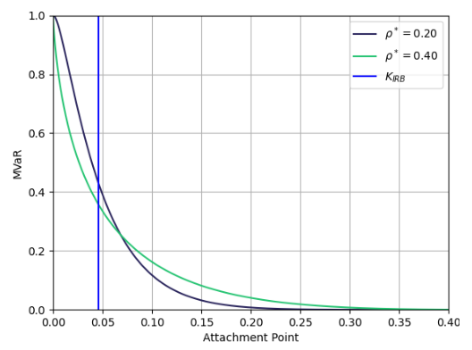
Note: Here MVaR denotes Marginal Value at Risk, and KIRB denotes securitisation capital for Internal Ratings Based approach.
3. Implementation
We estimate the capital requirement of the thin tranches using the parameters for the three different asset type namely (i) Small and Medium Enterprises (SME) (ii) Low Risk Weight Residential Mortgages, and (iii) Other Retail[1], European loan backed securitisation presented in Duponcheele et al. (2014). We also take a prudent correlation and default rate assumptions for the three different asset class, (i) SME, (ii) Residential Mortgage- Backed Securities, and (iii) Auto. These calculations form part of internal research for market monitoring and model calibration purposes.
The capital KIRB (Internal Ratings Based) required for the above risk parameters based on Basel Internal Ratings Based Approach (IRBA) formula is estimated using Basel Committee on Banking Supervision (BCBS) (2020).
The MVaR of the thin tranches are computed using equation 3.1 as proposed in Risk Control (2015). We take the confidence level as 99.9% consistent with the Basel III, thus α= 0.1%.
Φ−1(p[0]) − √ρ× Φ−1(α) ) pα = Φ ( (3.1) √1 −ρ
1 The other retail in this study is considered as auto loans.
Φ−1(pα) − √1 −ρ∗ × Φ−1 ( A LGD) ) MVaRTℎin Trancℎe = Φ ( √ρ∗
Here, Φ() represents the cumulative Gaussian function ‘A’ represents the attachment point of the thin tranche p[0] represents the pool default probability
We estimate the capital floor using equation (2.6), the risk parameters provided in Table 3.1, and different γ values. The γ is assumed between 1 to 2, which determines the attachment point of the senior tranche typically γ is found to be greater than 1.
Table 3.2 demonstrates the range of Capital floor for various γ across the three asset classes. The capital floor is correlated with the KIRB, for a lower K-IRB we observe a lower capital floor see RMBS against SME, irrespective of the attachment point of the senior tranche.
We further observe that the average capital floor as a percentage of the KIRB for the three asset classes are below 10% for γ 1.5 and 2 in both the RC Internal Research and calibration data (see Table 3.3). For SME loans with attachment point of 1.5 × KIRB, the capital floor is marginally above 10% but reduces by 50% when γ is 2, see Panel (b) of Table 3.3.
| RC Internal Research | Calibration Data | |||||||||||
|---|---|---|---|---|---|---|---|---|---|---|---|---|
| Asset Type | PD | ρ | ∗ ρ95% | Basel ρ | PD | LGD | Basel ρ | |||||
| SME | 1.59 | 15 | 20 | 17.41 | 0.94 | 45 | 19.50 | |||||
| RMBS | 1.31 | 15 | 10 | 18.23 | 1.08 | 25 | 18.99 | |||||
| Auto | 0.62 | 5 | 15 | 20.78 | 0.85 | 75 | 19.85 |
Note: All units are in percent. ‘RC Internal Research’ calculations are based on data and simulations conducted as part of our market monitoring and model calibration activities. K-IRB denotes capital requirement based on Internal Ratings Based (IRB) approach. The calibration data is based on Duponcheele et al. (2014). Here PD denotes probability of default and LGD denotes Loss Given Default.
| Asset Type | γ 1 1.5 2 | K-IRB | ||||||
|---|---|---|---|---|---|---|---|---|
| SME | 1.98 | 0.94 | 0.42 | 7.06 | ||||
| RMBS | 0.58 | 0.16 | 0.04 | 3.65 | ||||
| Auto | 0.11 | 0.03 | 0.01 | 7.82 | ||||
| Average | 0.9 | 0.4 | 0.2 | |||||
| γ | ||||||||
| Asset Type | 1 | 1.5 | 2 K-IRB | |||||
| SME | 1.24 | 0.60 | 0.28 | 5.70 | ||||
| RMBS | 0.47 | 0.13 | 0.03 | 3.37 | ||||
| Auto | 0.15 | 0.04 | 0.01 | 9.08 | ||||
| Average | 0.6 | 0.3 | 0.1 |
Note: Refer to the note under Table 3.1.
| Gamma | ||||||||
|---|---|---|---|---|---|---|---|---|
| Asset Type | 1 | 1.5 | 2 | K-IRB | ||||
| SME | 28.0 | 13.3 | 5.9 | 7.06 | ||||
| RMBS | 15.9 | 4.5 | 1.1 | 3.65 | ||||
| Auto | 1.3 | 0.3 | 0.1 | 7.82 | ||||
| Average | 15.1 | 6.1 | 2.4 | |||||
| Gamma | ||||||||
| Asset Type | 1 | 1.5 | 2 K-IRB | |||||
| SME | 21.8 | 10.6 | 4.9 | 5.70 | ||||
| RMBS | 13.9 | 3.9 | 0.9 | 3.37 | ||||
| Auto | 1.6 | 0.4 | 0.1 | 9.08 | ||||
| Average | 12.4 | 5.0 | 2.0 |
Note: Refer to the note under Table 3.1.
4. Conclusion
This note sets out the basis for a calibration of a floor on tranche capital based on analysis of the parameter uncertainty surrounding a key parameter in securitisation capital.
This parameter, which is denoted ρ∗, determines in the Pykhtin-Dev model and its multiperiod generalisation by Duponcheele, Perraudin and Totouom-Tangho (2013) how pool capital is spread across the different tranches of a securitisation.
We argue that model risk in pool capital (reflecting uncertainty in PDs and LGDs) is less appropriate as the basis for calibration since supervisory practices in Europe require banks to include Margins of Conservatism in estimates of these risk parameters.
Our findings suggest that for the asset cases we consider, a suitable floor is in the region of 10% of pool Risk Weights.
Reference
Basel Committee on Banking Supervision (2020) “Calculation of RWA for credit Risk,” CRE31, available at: https://www.bis.org/basel_framework/chapter/CRE/31.htm?inforce=20230101&published=20200327.
Duponcheele, Georges, William Perraudin, and Daniel Totouom-Tangho (2013) “Maturity Effects in Securitisation Capital: Total Capital Levels and Dispersion Across Tranches,” September, Risk Control mimeo, available at: https://www.riskcontrollimited.com//wpcontent/uploads/2015/02/Maturity_Effects_in_Securitisation_Capital.pdf.
Duponcheele, Georges, William Perraudin, Alexandre Linden, and Daniel Totouom-Tangho (2014) “Calibration of the CMA and Regulatory Capital for Securitisations,” April, Risk Control mimeo, available at: https://www.riskcontrollimited.com/public/Calibration_of_CMA.pdf.
Pykhtin, Michael and Ashish Dev (2002) “Credit Risk in Asset Securitisations: Analytical Model,” Risk, 15(5), S16-S20, May.
Risk Control (2015) “Default Probability Risk and Securitisation Capital,” April, available at: https://www.riskcontrollimited.com/wpcontent/uploads/2015/04/Default_Probability_Risk_Securitisation_Capital.pdf.
Risk Control Limited 13-14 Dean Street London W1D 3RS +44 (0)203 307 0730 www.riskcontrollimited.com