

Abstract
This paper develops a principles-based approach to calculating regulatory capital for securitisations. The approach is simpler and more transparent than the Basel Committee’s proposed Modified Supervisory Formula Approach (MSFA) and avoids the latter’s numerous opaque approximations. Importantly, our proposed approach is directly consistent with the Basel II Internal Ratings-Based Approach (IRBA) capital formulae for on-balance sheet loans. It is therefore “capital neutral” (at least, before model risk charges or other add-ons) in that a bank holding all the tranches of a securitisation will face the same capital charge as if it retains the securitisation pool assets as directly held exposures. Our suggested approach is therefore, less likely to encourage capital arbitrage.
SECTION 1 - INTRODUCTION
Good public policy in the field of banking regulation requires the adoption of appropriate rules for assigning capital to different banking assets. A key category of assets in this regard is that of securitisations. The market in securitisations played a central role in the recent financial crisis and, looking forward, could contribute significantly to banks’ efforts to secure stable funding post the crisis. It is particularly important, therefore, that capital rules for securitisation exposures be appropriately designed.
The Basel Committee has recently issued a consultative document on securitisation capital in the banking book. This document (BCBS (2012)) with its two supporting technical papers (BCBS (2013a) and BCBS (2013b)) sets out rules and capital formulae that substantively modify the rules included in Basel II (which were themselves set out in BCBS (2006)).
A major element in the proposed new rules is a set of formulae for capital termed the Modified Supervisory Formula Approach (MSFA). The MSFA is an attempt to calculate capital within a stylised theoretical model. That model is complex and inconsistent, in several respects, with the model used in Basel II for assigning capital charges to whole loans. The complexity of the model means that it cannot be solved in closed form. Hence, a sequence of approximations is employed in deriving capital formulae that are only roughly consistent with the purported underlying model.
An important feature of the MSFA is that is not capital-neutral. By this, we mean that a bank that holds all the tranches in a securitisation will be obliged to hold very substantially more capital under the MSFA than if, instead, it held the securitisation pool exposures directly. As securitisation practitioners, we consider that securitisation re-distributes credit risk but does not add or reduce credit risk. We, therefore, consider that well-designed regulatory capital arrangements should be neutral between situations in which assets are held directly or through structured products.
Note that, while we think neutrality should be built into the basic capital formulae, we recognise that concerns about model risk and possibly “agency risk”[3] may justify the inclusion of adjustments or over-rides. However, one should apply these transparently as additional charges or as conservative overlays on input parameters, rather than explicitly accept severe non-neutralities in the basic initial formulae employed.
In addition to capital neutrality, well designed securitisation capital formulae should satisfy other broad principles or axioms. These include transparency, consistency with other regulatory frameworks, and simple, parsimonious inputs with clear economic interpretations. We believe that the MSFA, in several key respects, fails to satisfy these axioms.
In this paper, we begin by discussing the basic principles that a satisfactory set of securitisation regulatory capital formulae should satisfy. We then proceed to develop and propose an alternative to the MSFA. Our proposed alternative approach is capital neutral and, in this sense, Arbitrage Free.
The Arbitrage Free approach is, in fact, a modified version of the Pykhtin-Dev model of securitisation capital. This model (exposited in Pykhtin and Dev (2002) and (2003) and surveyed in Pykhtin (2004)), assumes that the assets in the securitisation pool and the bank’s wider portfolio are driven by two imperfectly correlated common factors.
A common misconception is that this model necessarily implies less capital for a securitisation than does a model based on a single asymptotic factor. In this paper, we modify the Pykhtin-Dev model in an intuitively reasonable way so that capital neutrality is achieved while retaining compatibility with the Basel II ASRF model.[4]
Unlike the model employed in the SFA approach of Basel II or the MSFA approach currently proposed by the Basel Committee, the model we suggest may be derived in closed form. No confusing and unreliable sequence of approximations is, therefore, required to make it operational.
A key parameter in the model we propose is the additional degree of concentration that pertains within the securitisation pool compared to the bank’s wider portfolio. It is a matter of common sense that securitisation pools are in most cases more concentrated than a bank’s wider portfolio. This concentration may be reflected by assuming greater correlation between the risk factors driving the credit quality of securitisation pool assets than between the risk factors of assets in the wider bank portfolio.
Our approach consists of, first, maintaining the same correlation between securitisation pool assets and wider bank portfolio assets as assumed in the Basel II. This ensures capital neutrality. But second, we adjust a concentration parameter, thereby, allocating capital as required across tranches of different seniorities. Because the concentration parameter is related to genuine economic features of securitisations (unlike, for example the tau parameter of the MSFA), it may be set based on empirical evidence as well as to reflect regulatory judgments.
Note that several of the less justifiable features of the SFA and the MSFA stem from the need to avoid a cliff edge effect that arises when securitisation capital is analysed in a singlerather than a two-factor model. In particular, both the counter-factual assumption of uncertainty in attachment points and the expected shortfall approach adopted in the MSFA (which introduces an inconsistency with the Basel II IRB capital formula) represent attempts to get around the cliff edge drawback of the single risk factor model. When a two factor model is employed, this issue is immediately resolved through an appropriate setting of the concentration parameter.
The remainder of this paper is arranged as follows. Section 2 discusses the axioms or principles that we believe should guide the derivation of a suitable model for securitisation regulatory capital. Section 3 analyses the MSFA and shows in what respects it deviates from our axioms. Section 4 sets out notation and assumptions and discusses the Basel II whole loans capital formulae. Section 5 derives capital for securitisation tranches under our proposed approach. Section 6 discusses empirical calibration of our proposed approach. Section 7 presents illustrative calculations using different capital formulae. Section 8 looks at possible extensions and work remaining. Section 9 concludes. Appendices provide derivations, information on calibration methodologies and analysis of approximations employed in the MSFA.
SECTION 2 - PRINCIPLES FOR SECURITISATION REGULATORY CAPITAL
In this section, we set out the basic principles that we believe should be followed in devising capital formulae for securitisations. We think it is important in designing regulations to identify such principles and then to apply them consistently.
Principle 1: (Objective statistical basis) Capital for securitisation exposures should be based on their marginal contribution to a single, widely accepted statistical measure of the bank’s total portfolio risk.
Principle 2: (Neutrality) Apart from model risk charges, the capital a bank must hold against a set of assets should be unaffected by packaging these assets into securities.
Principle 3: (Regulatory control) Control parameters should be available that permit regulators and supervisors to achieve their objectives and exercise judgments in the allocation of capital across different types of exposure. Such parameters should reflect the economic reality of transactions so that they could in principle be calibrated from empirical data.
Principle 4: (Transparency) Capital formulae should reflect in a simple way the nature of risk and be consistent with other regulatory capital approaches to facilitate comparisons and to promote transparency.
These principles reflect different considerations in the design of capital requirements for securitisations.
On Principle 1, the prime candidate here for banking book calculations is for capital to be based on Marginal Unexpected Loss criterion, i.e., that capital of an exposure should equal a) its marginal contribution to the Value at Risk of the Bank’s wider portfolio less b) its expected loss, adjusted for c) a model risk charge.
The Marginal Unexpected Loss Approach is a widely adopted standard employed throughout banking, insurance and other finance industry sectors. It is the basis for whole loan capital charges in Basel II and it would be strange not to adopt it in the determination of securitisation capital.
On Principle 2, in the context of securitisations, this implies that capital should be the same if the exposures are held directly or indirectly by a bank which owns all the tranches in a securitisation. Capital arrangements that do not respect neutrality are prone to encourage capital arbitrage or to divert financial activity to different channels. Even if overrides and model risk adjustments are adopted which detract from neutrality, we believe that, in the interests of transparency, they should be explicitly imposed on top of a capital neutral set of approaches.
Principle 3 recognises the need for regulators and supervisors to make judgements reflecting risk and other considerations that are, for whatever reason, inadequately reflected in the basic capital formulae.
Principle 4 should be uncontroversial. The basis and justification for capital charges should be straightforward and easy to comprehend for regulated firms and regulators alike.
SECTION 3 - THE MSFA: A RULE-BASED MODELLING APPROACH
The Modified Supervisory Formula Approach (MSFA) has been proposed by the Basel Committee as a successor to the Supervisory Formula Approach (SFA) previously employed as part of the framework for securitisation regulatory capital. In this section, we shall set out the basic features of the MSFA (focussing on how it departs from the SFA) and then consider how the MSFA measures up to the principles identified in Section 2.
Under the MSFA, capital for a given tranche exposure is based on a Marginal Expected Shortfall (MES) measure. The MES is defined as the marginal contribution of the tranche exposure to the Expected Shortfall of the Bank’s wider portfolio. Here, the Expected Shortfall, is defined, in turn, as the expected loss on the Bank’s portfolio given that the portfolio has deteriorated beyond a given quantile of its distribution.
Note that this approach departs from that followed more generally in the IRB banking book approach. In this latter approach, capital for an exposure is based on its marginal contributions to the Bank’s wider portfolio Unexpected Loss, i.e., the Value at Risk minus the Expected Loss.
This change seems to us wholly regrettable as it immediately builds into the framework inconsistencies between the regulatory capital for on and off-balance sheet holdings of the same exposures and hence makes neutrality impossible except in a very approximate sense.
One of the stated justification for the shift to an Expected Shortfall approach appears to have been the desire to mitigate the so-called cliff-edge effect. The cliff edge effect refers to the fact that capital on mezzanine tranches in the SFA approach may decline swiftly as seniority increases. Efforts were made to mitigate this effect in the SFA by introducing the counterfactual assumption that significant uncertainty existed around the location of attachment points in securitisations.
As we argue below, however, there are alternative and superior ways of removing the cliff edge effect and hence altering the basic assumptions of the capital framework and thereby sacrificing neutrality appears to be ill-advised.
The fact that the MSFA chooses to include rather than to subtract expected losses from its basic Marginal Expected Shortfall risk measure also has major implications. Note that the MSFA includes Expected Losses in a super-conservative way in that (i) they are expected losses for a period equal to the minimum of five years or the maturity of the deal and (ii) the Expected Losses are calculated inclusive of a risk premium (at least for all except the first year). For some securitisation exposures, the Expected Losses easily exceed the Unexpected Losses allowed for in the MSFA.
A second major difference between the MSFA and the SFA that preceded it is a different approach to tackling what has variously been called a maturity or “mark-to-market” adjustment. In the IRB banking book capital formulae for on-balance sheet loans, the capital for a loan is based on a calculation of its marginal contribution to the VaR of the Bank’s wider portfolio over a one-year horizon and then scaled up by a maturity factor.
The use of regulatory capital formulae based on default mode models[5] has confused many in the regulatory community and in the industry who have believed that the Basel framework was conceived of as a “default mode” approach. In fact, the capital framework was originally calibrated using economic loss-mode ratings-based models and employing portfolios of loans with maturities longer than the 1-year horizon of the VaR calculation.
The one-year, default-mode marginal VaR formulae that appear in the Basel II rules for corporate loans were just a reasonable fit (when accompanied with simple maturity adjustment factors) to the intended capital levels which had previously been calculated in a multi-period, ratings-based framework.
In this sense, the fact that the on-balance sheet loans capital formula includes a maturity adjustment means that the capital is already adjusted for “mark-to-market” effects. One might question the magnitude of the adjustment but it is undeniably already present.[6]
In the SFA securitisation capital formulae employed in Basel II, again a notional default mode formula was developed and this is used to “distribute” a total amount of capital among different tranches. But the key point to grasp is that since the capital distributed is based on the IRB formula for on-balance-sheet loans, it already includes a maturity or “mark-tomarket” adjustment.
The presentation of the MSFA (if not the modelling in the MFSA itself) reflects some of the confusions mentioned above about whether the Basel approach was default or economic loss mode. BCBS (2012) states: “The Committee is proposing to amend the SFA to incorporate a maturity effect at the tranche level. This change is intended to make the MSFA more consistent with both the IRB framework and the revised RBA approach, which also incorporate a maturity adjustment.” But, the SFA already includes a maturity or mark-tomarket adjustment because one of its inputs is KIRB, the on balance sheet capital for the underlying assets which is adjusted for maturity so including a tranche level maturity adjustment does not make the securitisation framework more consistent with the IRB framework.
Again, the regrettable implication of attempting a separate maturity adjustment in a complex, non-closed-form model (rife with numerical approximations) like the MSFA is to obtain a framework which bears little relation and hence yields quite different capital for securitisations that one obtains from the on-balance sheet approach.
Having made the above two general comments on the MSFA, we now provide more detail on how the capital formula is constructed. An expression is derived for the marginal Expected Shortfall associated with a given securitisation tranche. This involves the conditional expectation of an integral of the distribution of losses on the underlying pool. Manipulating this, one obtains a general expression involving a conditional loss distribution under risk neutral assumptions (so as to reflect risk aversion). Principle How the Modified Supervisory Formula Approach Performs
1. Objective The MSFA follows a clear statistical criterion for risk but this differs from the statistical criterion employed elsewhere in the IRB approach, namely Unexpected Loss. basis The over-rides, smoothing parameters and the modelling inconsistencies mean the MSFA is only tenuously connected to unexpected loss. The MSFA may, therefore, be regarded as a distributive function of inconsistently calculated capital which departs fundamentally from the IRB banking book capital formulae.
Unfortunately, this distribution is not available in close form so an approximating beta distribution is substituted for the actual distribution. The mean and variance of losses are calculated (with several layers of approximation) and substituted into the beta distribution. Several of the approximations which have significant impacts on are adopted with relatively little comment in the Basel Committee documents. No sensitivity analysis is reported of what is the effect on capital for different tranches of using approximations instead of the true model.
Once the capital formula has been evaluated a set of regulatory over-rides familiar from the SFA are imposed. Thus, the MSFA (like the SFA) deducts capital to all tranches detaching below a threshold (Pool IRBA capital including EL) and then distributes an additional markto-market capital above this threshold based on a parameter ‘tau’ and a smoothing function with parameter ‘omega’. Finally, a “model risk” charge is introduced in the form of a fixed floor (160 bps in the MSFA, 56 bps in the SFA), disconnecting the capital charge from the underlying asset risks.
Returning to the principles we advocated before that should guide the development of regulations on securitisation capital, we summarize in Table 1, how the MSFA performs.
To conclude, the capital charge formulae presented in BCBS (2013a) are only tenuously connected to the underlying model and this model departs from the on balance sheet approach to capital in crucial respects. The framework is opaque, over-engineered and, crucially, ignores the basic need of a set of capital regulations that, with the proviso of allowing for model risk, packaging into securities should not alter required capital. The MSFA approach may be characterised as “rule-based” (with highly questionable rules) rather than “principlesbased” in that it adopts a series of approximations and then adds successive overlays, and caps to cope with the unreasonable outcomes that arise. A simpler more transparent approach that respects the principles listed above would be much preferable.
SECTION 4 – REVIEW OF THE IRB LOAN CAPITAL APPROACH
Below, we develop an approach to modelling securitisation capital that respects the principles listed in the previous section. The approach must be based on a clear statistical risk criterion, must yield capital neutrality compared to on balance sheet exposures, must afford regulators enough discretion through the use of economically motivated control parameters and must be transparent and simple to understand and apply.
Neutrality and transparency dictate that the framework developed must be closely related to the existing framework for calculating capital for exposures on balance sheet. We start by briefly reviewing this approach.
The statistical criterion employed is unexpected loss, i.e., Marginal VaR of an exposure within the Bank’s wider portfolio less the expected loss. To derive this, it is supposed that each individual exposure defaults over a one year period if its associated latent variable falls below a threshold. The latent variables for individual exposures are assumed to be standard Gaussian and to have a single standard Gaussian common factor, denoted . The latent variable for the ith exposure, , may be expressed as: (1) = ∙ + 1 − ∙ ,
i Here, is a fixed parameter, while , is standard Gaussian and mutually independent j ≠ i . from and uncorrelated with and with , for any j ≠ . Hence, is the correlation between and for any
Conditional on the common factor, the probability of default of the ith exposure may be written as[7]:
(2) ∙ !"#$% & '
be derived simply using the insight of Gourieroux and Scaillet (subsequently developed and Here, () is the unconditional probability of default. The marginal VaR of the exposure may applied by Taasche and Gordy). These authors point out that the expected loss on an individual exposure conditional on the portfolio being at its α-quantile equals the Marginal VaR at a confidence level α.
In the present context, the marginal Unexpected Loss of the ith exposure (MULi), therefore, equals
(3) ∙ 2 & *+, = *-./ − 0, = ,1) ∙ ' − ,1) ∙ ()
given default on the exposure. The Basel II IRB framework employs the above expressions, Here, &3 is the α-quantile of the standard Gaussian distribution and ,1) is the loss setting α= .0001 class and the rating of the exposures.[8] and employing different correlation parameters, , depending on the asset
There are two adjustments made to the above by the Basel II IRB framework. First, the above calculation is appropriate for one-year exposures or if risk calculations are conducted on a default mode basis in that the only risk considered is defaults over the one year horizon. Loans with maturity longer than one year may change value because credit ratings migrate without a default occurring. An economic loss concept of risk will take this into account. The Basel II IRB capital charge formula takes into account maturity by scaling the unexpected risk by a maturity adjustment factor. For corporate exposures, this scaling factor takes the form: D (4) &89 :.< ∙=>.&&?<: >.><@A?∙B C D ' & &.<∙=>.&&?<: >.><@A?∙B C *.4567 = For retail exposures, the scaling factor is omitted. This is justified by the fact that most retail exposures have short maturity. For residential mortgage exposures, an adjustment was made 7 Where stands for the normal distribution function and & stands for the reverse normal find in empirical research on mortgage defaults over a year and hence, implicitly, represents a by including a correlation of 15%. This value is substantially greater than one would ever simple maturity adjustment.
The second adjustment made to the above by the Basel II IRB framework is to include a model risk adjustment, scaling up the total capital implied by the formula by 6%.
marginal contribution to the Value at Risk of the Bank’s wider portfolio less b) its expected To be precise, the capital requirement of an exposure in IRB, denoted R/ST,, equals a) its loss, adjusted for c) a model risk charge: R/ST = *-./′ −0,′ + */R′ where *-./V = *-./ × *.4567 and 0,′ = 0, × *.4567 ; and */RV = 6% × *+, × *.4567 = exposures. Note that this formulation is consistent with Principle 1 as specified above. 6% × XST with *.4567 as in equation (4) for corporates and equal to 1 for retail
SECTION 5 – A PRINCIPLES-BASED APPROACH TO SECURITISATION CAPITAL
We now turn to the derivation of a capital formula for securitisations that respects the principles established earlier. To ensure neutrality, it should be the case that, before model risk adjustments and over-rides are taken into account, capital for a bank that holds all of the tranches should equal the capital it would have to hold on the underlying securities.
To ensure this, we adopt the following assumptions. Consider a pool of loans held by the Special Purpose Vehicle of a securitisation. We again assume that each individual loan defaults when an associated Gaussian latent variable falls below a threshold. We express the latent variables in the following way.
(5)
(6) = + 1 − = ∗ YL Z + 1 −∗ [ Here, YL Z is presumed to be a factor common to all the exposures in the SPV pool but orthogonal to the common factor driving the bank portfolio, namely: . Substituting, one may define the following expressions:
(7)
(8) =& , \\B L Z + 1 − , \\B [ (9) L Z = ,]^^_ = + 1 − ∗ YL ZC , \\B = + 1 − ∗ There are several points to make about these assumptions.
class by Basel II and if the exposure is small compared to the wider bank portfolio, then the First, if the correlation parameter, , takes the value prescribed for exposures of this asset exposure’s unexpected loss will equal the value assumed under Basel II.
pairwise correlations than with those of exposures in the wider bank portfolio. This greater Second, if ∗ > 0, the latent variables of individual exposures within the pool have higher risk concentration within the SPV pool may be justified on common sense grounds. It is clearly true that SPV pool assets are in almost all cases more specialised in asset class or geographical location than those of a bank’s entire portfolio. Occasionally, balance sheet structured products are constructed that are highly diversified and designed to mimic in coverage a bank’s broader portfolio but even here there is almost always some focus on a set of vintages or some asset class.
Third, assumptions very similar to these have been proposed already in Basel II discussions in the analysis of double default risk (see Heitfield and Barger (2003))[9]. In this case, the latent variables for an obligor and a guarantor are assumed to be more correlated with each other than either is with other comparable exposures in the bank’s wider portfolio. The idea is to allow for wrong-way risk. The effect is very similar to what we propose for securitisations in that assets are assumed to be exposed to ‘common’ shocks over and beyond those associated with the systemic risk.
Fourth, as a two factor, latent variable model of securitisation risk, quantities such as expected losses, marginal VaR and unexpected losses may be derived as in the Pykhtin-Dev model exposited in Pykhtin and Dev (2002) and (2003) and surveyed in Pykhtin (2004).
In that model, consider a pool of one-year, homogeneous[10], infinitely granular, non-interest-
and total par equal to unity held by an SPV. Since the exposures are presumed to be bearing loans with individual default probabilities of (), fractional expected losses of ,1), homogeneous, we drop the subscript for exposure i. The SPV has issued pure discount notes also with a total par value equal to unity. Suppose the notes consist of a continuum of thin tranches.
If losses on the pool exceed the attachment point A of a marginally thin tranche, that tranche will default and the recovery rate will be zero. Hence, expected losses on the tranche equal the default probability of the tranche which in turn equals the probability that losses on the pool exceed the attachment point A. So, in the notation employed above, expected losses on the tranche equal:
(10) & ]^^_ ∙ Jijkh M 0,bc bdecf5 = ()bdecf5 = g ]^^_ l
9 In this model, the latent variables of an obligor (m) and a guarantor (n) are specified as:
To obtain the expected losses of a discretely thick tranche with attachment point A and detachment point D, one must integrate the above expressions for the marginally thin tranche from A to D. This is simple to accomplish numerically but closed form solutions are also available.
One may express the expected loss on a discretely thick tranche in terms of expected loss on two senior tranches. A senior tranche is a tranche with a given attachment point X and a detachment point of unity. The expected loss on discretely thick tranche may be expressed in terms of the expected loss on senior tranches as follows:
1(− A) × ELSeniorTranche(A) − 1(− D) × ELSeniorTranche(D) ELThickTranche(A, D) = (11) D − A
The above expression depends on the expected loss for a senior tranche, denoted ELSeniorTranche (X ) . (Here, X is the attachment point). This in turn may be obtained by integrating the thin tranche formula. The result (see Appendix 1 for more details) depends on
steps, with X being an attachment point: :, , the bivariate cumulative standard normal distribution function[11] with the following × − × LGD N[2] X PDTranche(X ) ELSeniorTranche(X ) = 1− X
−1 −1 N[2] ≡ N[2](N (PD), N (PDTranche(X )) , ρPool ) (12)
![Equation: −[1] −[1] X N (PD) − 1− ρPool ⋅ N LGD PDTranche(X )= N](/api/media/file/eq-8-300x53.png?prefix=media)
ρPool

To calculate the marginal VaR (at an α-confidence level) of a thin tranche held within a wider bank portfolio, following the Gourieroux-Scaillet insight, one may calculate expected
quantile. losses conditional on the common factor driving the bank portfolio, , equalling its α- Conditional on equalling its α-quantile, the default probability of pool exposures is: −1 −1

− ρ

Conditional on equalling its α-quantile, the pairwise correlation between pool assets is: −[1] Cov(Zi , Z j | YBank = N (α)) * (14) ρPool,α ≡ −1 −1 = ρ σ(Zi |YBank = N (α))⋅σ(Z j |YBank = N (α))
respectively, yields expressions for the thin and thick tranche marginal VaRs. Replacing () and \\B where they appear in equations (10) and (12) with ()[2] and \\B,2,
Note that in the expression for thin-tranche capital in Equation (10), if () is replaced with the ratio is positive and zero otherwise (as the ratio approaches either positive or negative ()[2] and if \\B is replaced with ∗, then as ∗ →0, capital equals unity if the numerator in infinity). This is the cliff edge result that motivates much of the model development in the MSFA and which is avoided simply by assuming ∗ > 0. Also, note that, apart from maturity and model risk adjustments, ()[2] × ,1) equals the Basel consequence of the capital neutrality properties of the approach we advocate. II XST + 0,′ (the expected loss inclusive of maturity adjustment). This is a simple
Figure 1 shows the expected loss on a tranche (the integral under the red curve) and the unexpected loss (the integral under the blue curve minus that under the red curve). The marginal VaR (the integral under the blue curve) may be thought of as a stressed expected loss. The capital requirement is the difference between those 2 curves (each being a simple Vasicek loss distribution).
In developing the capital formulae exposited above, we did not discuss the issue of SPV pools that contain heterogeneous exposures. Since all realistic cases have this property, the issue clearly requires attention. Two approaches are possible:
• Option 1: the most straightforward approach is to use ()[2] = XST + 0,′)/LGD where XST is the Basel II IRB capital for the pool assets (inclusive of maturity LGD is the total estimated mean loss given default for the pool assets. This approach adjustment). 0,′ is the total pool expected loss inclusive of maturity adjustment and could have the disadvantage that “bar-bell” type structures might potentially be constructed to arbitrage this type of approach.
• Option 2: an alternative might be to calculate capital requirements for each individual underlying pool asset by calculating the PD, LGD, stressed PD and stressed LGD for a tranche that solely contains identical assets. This is a way of permitting heterogeneity in the pool. In the second option, one would define the weight t of an asset u in a pool, with a pool size vw vw ]^^_. The capital requirements for the ith asset would then be 05) \\B is given by: t = but using the input parameters of the single pool exposure in question. Again, a model risk set equal to the product of t and of the capital based on the expressions derived in Section 5 premium of 6% of the pool risk weight could be added. Such implementation is proposed in Appendix 4. We intend to carry out further work to evaluate whether this approach gives a reasonable approximation to the actual (exact) capital requirement of a deal with a heterogeneous pool.
economically reasonable notion that defaults of exposures within structured product pools are A key parameter in the proposed model is the ∗ parameter. This parameter captures the typically more highly correlated than those found within a bank’s wider portfolio[12]. By not having this assumption in the existing securitisation framework (and in the revised securitisation framework proposal), there is an implicit and incorrect assumption that the pool of assets in the SPV is just as diversified as the bank’s wider portfolio.
pool is as diversified as the wider bank portfolio), the model reduces to the single risk factor As noted in the discussion after equation (14), when ∗ is set to zero (i.e. when the SPV asset model and marginal capital for thin tranches exhibits the cliff effect that the SFA and MSFA make such strenuous efforts to avoid. The cliff-effect may be eliminated within an economically reasonable framework (and without resorting to artificial smoothing techniques) by allowing ∗ to be positive. A particularly important feature of the approach just described is that it generates regulatory capital for a bank that holds all the tranches of a securitisation equal to the Basel II capital it would be required to hold if it held all the underlying assets. Additional model risk charges and minimum capital ratios might be added but the basis framework is capital neutral. For this reason, it seems reasonable to label the proposed approach the Arbitrage-Free Approach or AFA.
Note that the framework just described does not contain an explicit mark-to-market adjustment. But there is no need for one. The Basel II charges for underlying assets already contain a maturity adjustment which is entirely equivalent. Including an additional maturity
diversified pools. In Moody’s methodology for corporates, there are correlation add-ons for concentration leading to a total intra-sector correlation of up to 15%, as well as over-concentration correlations.
adjustment at the tranche level would be double counting. This is why it would have been logically inconsistent to include a tranche level maturity adjustment in the original SFA.[13]
We turn, finally, to an evaluation of how the approach just proposed measures up to the principles we described earlier. We summarize in Table 2 the results of the evaluation.
* SECTION 6 – EMPIRICAL EVIDENCE ON THE ρ PARAMETER
An important gap in the model proposed above is a demonstration of what value the
securitisation compared to the correlation allowed for in the Basel II assumptions. parameter, ∗, should take. This parameter reflects the additional intra-pool correlation in the
If we assume that the individual exposures within structured product pools have the same correlation with exposures in the wider bank portfolio as are prescribed in the Basel framework and we possess estimates of the correlation between the two common factors
incremental common factor risk in the securitisation pool.[14] driving the bank portfolio and the securitisation pool, it is possible to identify ∗, the
To state this more formally, from equations (8) and (9)
ρ ρ Correlation (YBank ,YSPV ) ≡ ρS,B = = * (15) ρPool ρ+ 1(− ρ) ρ Squaring and rearranging yields:
ρi (1− ρS,B ) * ρ =[2] (16) ρS,B (1− ρi )
bank and securitisation credit quality. Hence, we may infer ∗ from measuring the correlation between the common factors driving
One way to approach this is to model ratings transitions. There is a long-standing literature motivated by the problem of parameterising correlations in portfolio credit risk models that attempts to estimate correlations for the latent variables driving the credit quality of obligors from different sectors. Contributions include Gupton, Finger and Bhatia (1997), de Servigny and Renault (2003), Moody’s (2004), van Landschoot and Jobst (2007) and Perraudin and Zhou (2012).
In this section, we employ the Kendall’s tau method presented in Moody’s (2004) and the
provides details of the methodologies employed.) From these estimates, we then infer Maximum Likelihood approach of Perraudin and Zhou (2012) to estimate L,. (An appendix estimates of ∗. The most obvious way to proceed might seem to be to estimate the asset correlation for bank and securitisations from transitions in their respective ratings. However, bank ratings were much less volatile than securitisation ratings through the crisis period. We believe this partly reflects the fact that banks in many countries were supported by their national authorities throughout this period and hence volatility in the credit quality of underlying bank portfolios was not directly reflected in changes in ratings. Hence, bank ratings data are not directly useful for our purposes. 14 Note that one could attempt a more “bottom up” approach to calcibrating ∗ by estimating pool correlations
Instead, we think it is reasonable to regard the common factor driving securitisations as equivalent to the common credit market factor presumed in Basel II. To estimate the correlation between this factor and the factors driving individual securitisations, one may then focus only on the correlation between the latent variables driving securitisation ratings. Using the methods described in the Appendix, we may estimate this correlation in a relatively simple fashion.
Table 3 shows the results of our estimations of correlations between individual
pairwise correlation between the latent variables driving the ratings of two entities within a securitisations. We may denote this pairwise correlation as L,L. Each entry shows the given sector based on a particular sample (differentiated by period and geographical region).
We report results for six individual sectors (rows 1 to 6 in the tables of results) and for the market as a whole (row 7 in the tables). The six sectors were based on the Moody’s definitions of high level structured product sectors. The precise breakdown of these sectors may be obtained from the authors upon request.
The results obtained using the two estimation methods we implement show some variation. The Kendall’s tau method typically yields lower correlation estimates. Sensitivity analysis reported in Moody’s (2004) suggests the Kendall’s tau method may suffer from bias when correlations are high so we prefer to focus on the Maximum Likelihood results.[15]
As noted above, to infer ∗, we suppose that the correlation between the bank and the securitisation with the common factor driving the whole category of securitisations, which securitisation factors, L,, equals the correlation between the latent variable driving a single implies that:
ρ (1− ρ ) * i S,S ρS,B = ρS,S and so ρ = (17) ρS,S (1− ρi ) On this basis, the ∗ estimates are as shown in Table 4.
estimates from Table 3. A reasonable approach is to use the Maximum Likelihood results for The results in Table 4 show ∗ based only[16] on individual Maximum-Likelihood-based
between 3 and 10%. all structured products shown in the last line of Table 4. This would imply ∗ values of
estimate the degree of correlation in SPV pools and compare this to the degree of correlations Note that one could follow other approaches in calibrating ∗. For example, one could within a broader bank portfolio. Another possibility might be to look at the correlation assumptions adopted by ratings agencies in securitisation rating analysis and to compare this to correlations specified in the Basel II on balance sheet rules. In future work, we intend to explore these alternative approaches.
Maximum Likelihood based estimates
It is important also to recognise that, if our approach were used as the basis for regulatory capital calculations, while the chosen value of ∗ might be informed by empirical evidence, it would offer regulators an important source of control. Increasing ∗ has the effect of more conservative in the treatment of senior versus mezzanine tranches. allocating more capital to senior tranches. Regulators may wish to increase ∗ in order to be
16 The Kendall’s tau-based estimates for ∗ are very high reflecting the fact that the Kendall’s tau-based
SECTION 7 – NUMERICAL EXAMPLES
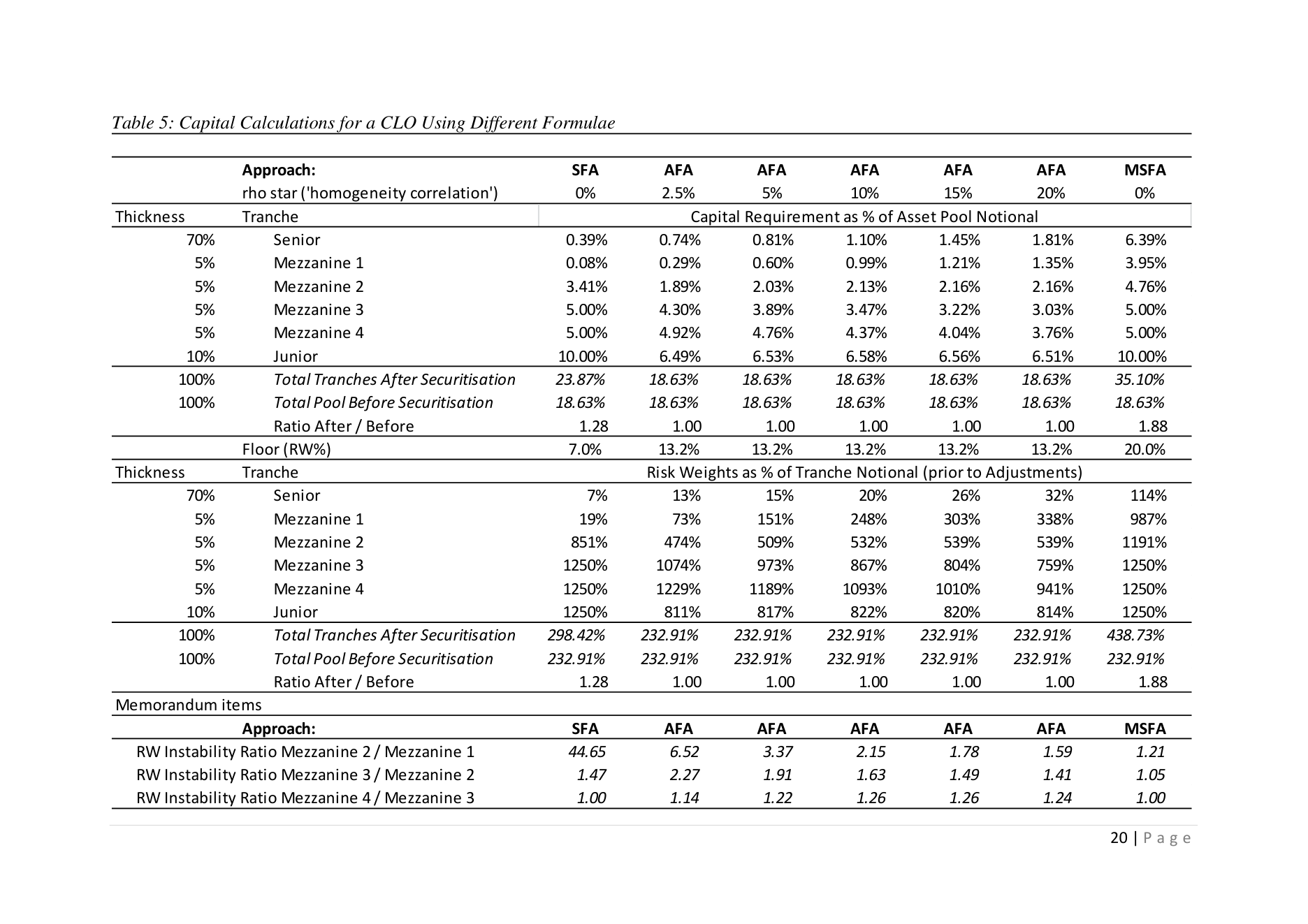
In this section, we compare outcomes for capital calculations using different capital formulae. The basis for the calculations is two typical securitisations. The first of these involves a pool of European corporates (both SME and Leveraged Loans). Characteristics of the pool exposures are: () equalling 5%, ,1) equalling 55%, maturity of 5 years, systemic correlation equal to 13%. The pool is highly granular. Key implied quantities for the pool maturity adjustment in equation (4). are: 0,V = 3.75% and *-./V = 21.33% (in both cases, these have been scaled up by the
The results of the calculations are shown in Table 5. Results for the AFA are presented for
compared to the on-balance sheet capital. The MSFA, on the other hand, approximately different ∗ values. As may be observed, the total capital is somewhat boosted by the SFA doubles the level of capital. The sensitivity of the capital charges generated by the SFA to seniority in the mezzanine area of the structure (i.e., the quasi-cliff effect) is apparent. While this sensitivity is eliminated by the MSFA, it is also very substantially reduced if the AFA is employed.
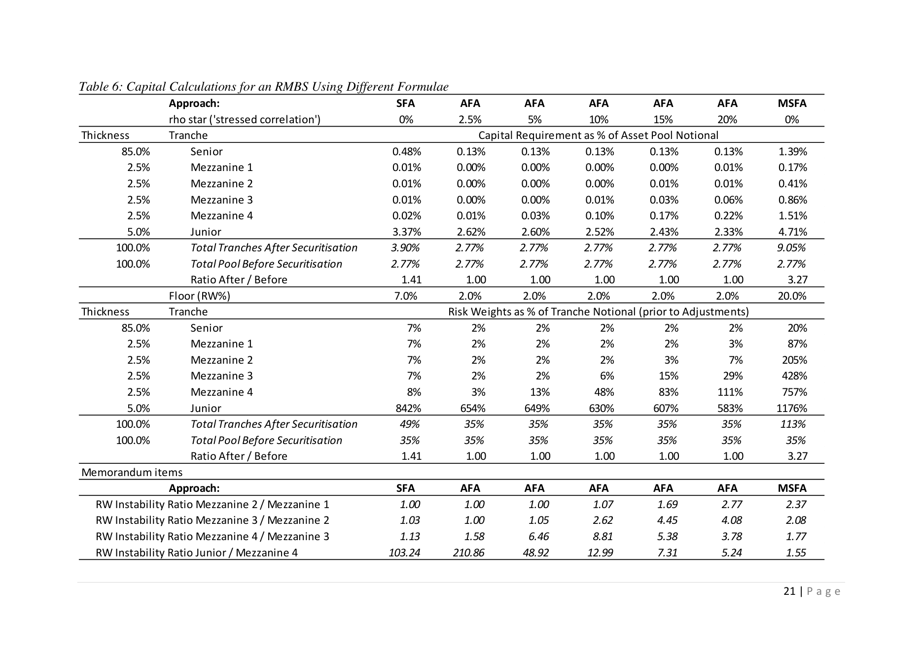
Table 6 shows results comparable to those contained in Table 5 but this time for Residential Mortgage Backed Securities with high credit quality pools. In this case, the parameters
correlation equal to 15%. The pool is highly granular. Key implied quantities for the pool are: assumed are: () equalling 1.5%, ,1) equalling 20%, maturity of 5 years, systemic 0,V = 0.3% and *-./V = 2.91%. In this RMBS transaction, the SFA implies total capital equal to 141% of the presecuritisation capital whereas the MSFA implies capital of 327% of the pre-securitisation amount. Again, the higher instability ratios encountered with the SFA are reduced by the AFA although not by as much as with the MSFA.
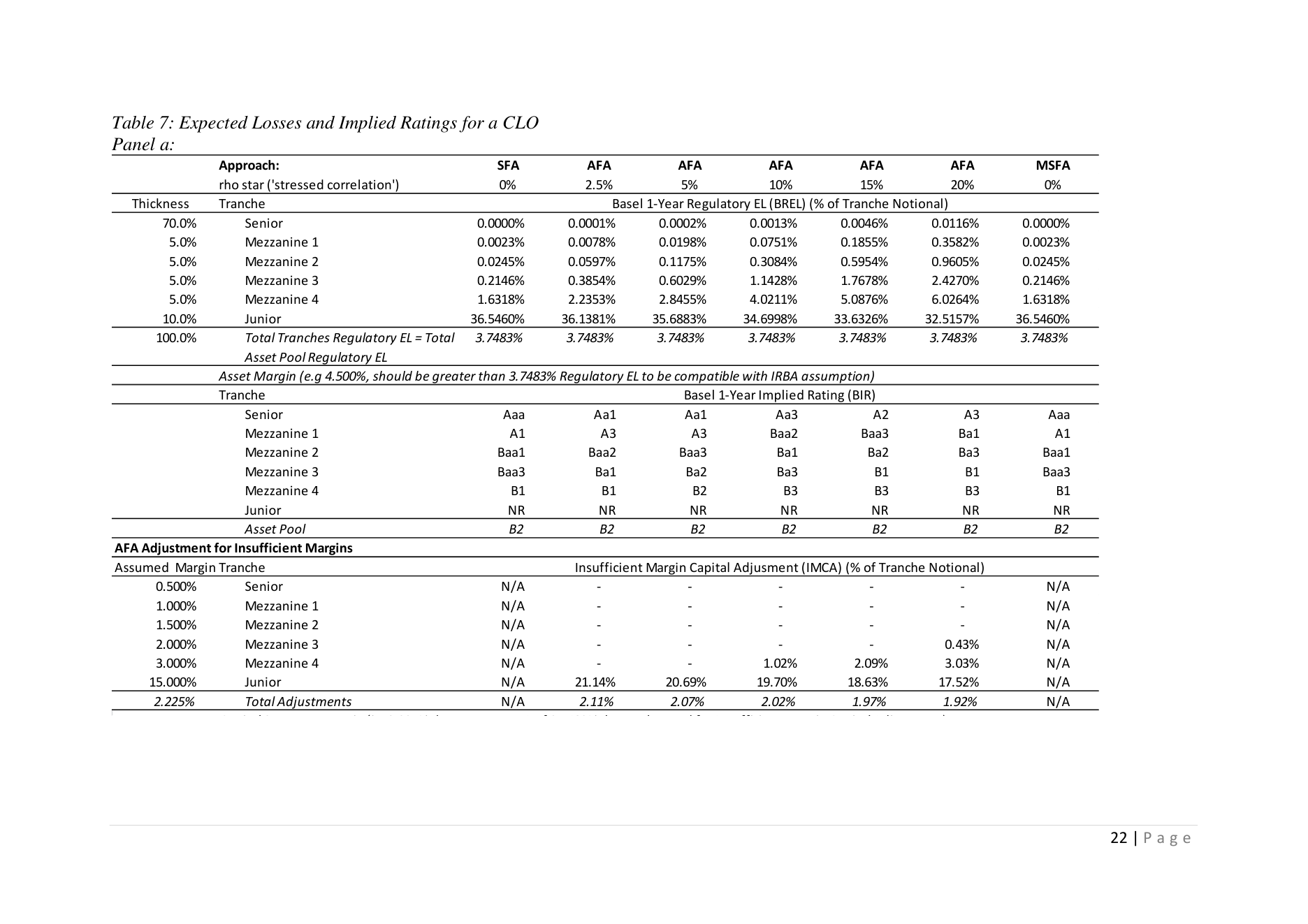
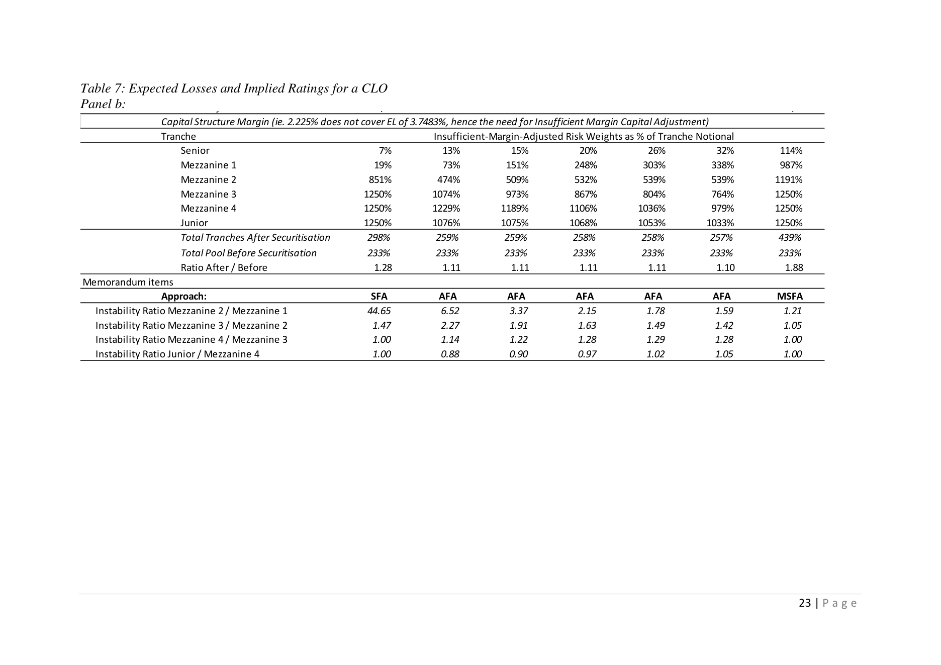
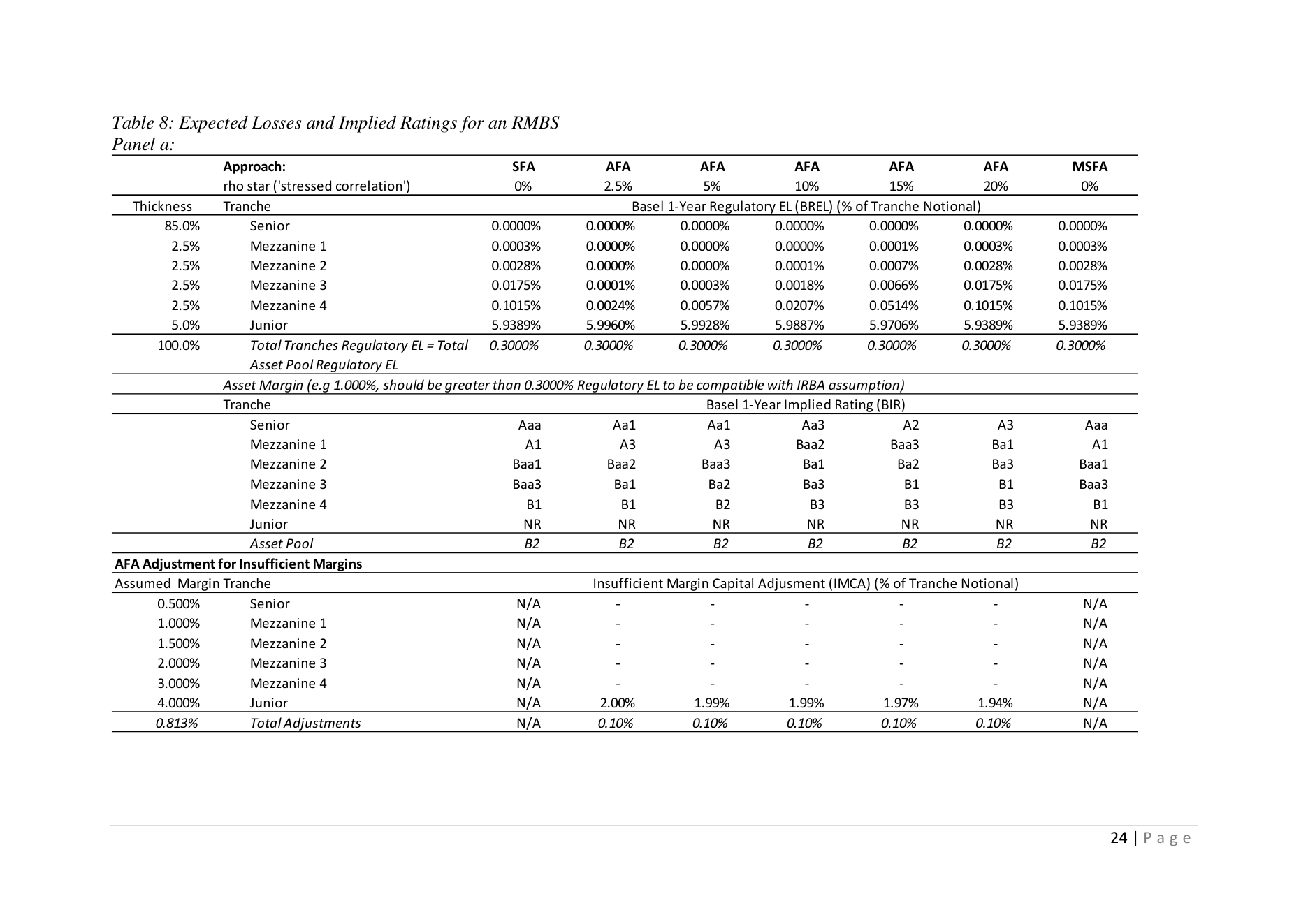
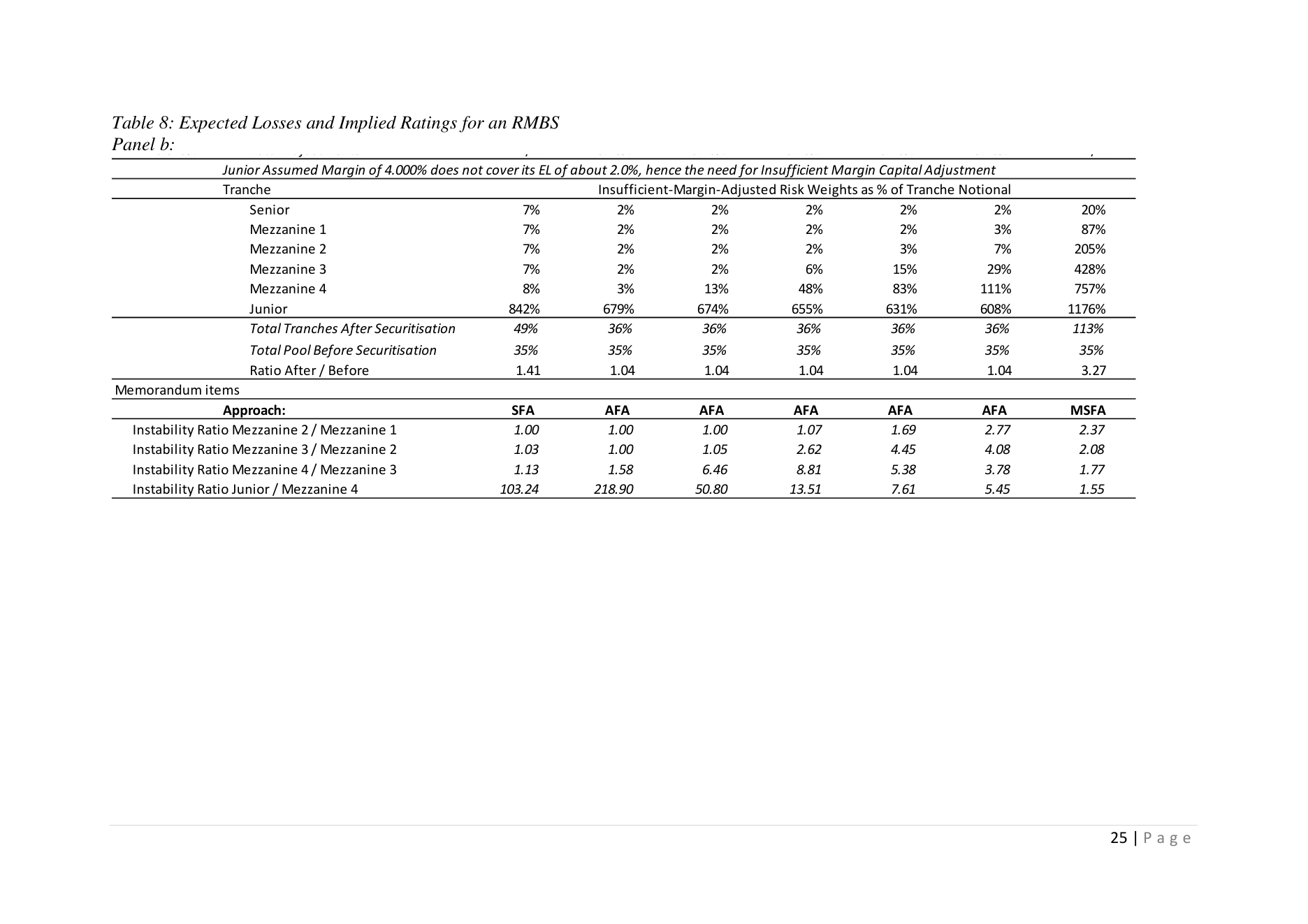
affects expected losses of different tranches and their implied ratings. The distribution of Tables 7 and 8 show, respectively for the CLO and the RMBS examples, how changing ∗
calibrate a revised Ratings Based Approach by fitting the actual ratings of real transactions. expected losses across tranches and the implied ratings could be used to calibrate ∗ or to
The results in Tables 7 and 8 also show the effects of augmenting capital when the spread on a tranche is insufficient to cover the tranche’s expected loss. The IRB approach explicitly assumes that future margin income is sufficient to cover one-year expected losses. We propose that this assumption be checked and, where it is not true, an adjustment be made. This suggestion is explained in greater detail in Section 8.
SECTION 8 – OTHER DISCUSSION POINTS AND WORK REMAINING
In this section, we discuss possible extensions and work remaining.
Adjustment for Insufficient Tranche Margin
The Basel II framework calculates the Unexpected Loss contribution by deducting from the VaR contribution the Expected Loss contribution. The justification for this is the assumptions that the Future Income Margin is sufficient to cover the expected loss over the regulatory horizon.
It would seem reasonable that this approach be applied to securitisation tranches as well as loans as tranches are equally assets of the bank. If the spread margin of the tranche is insufficient to cover its expected loss over the regulatory horizon, an upward adjustment could be made in that the capital charge would rise by: z.{|}.~ℎG 0{G4G6 ,m −|}.~ℎG I}G.6 *.}nu~ , 0 Note that this would represent a deviation from the Basel II capital for on-balance sheet loans and hence a relatively minor deviation from capital neutrality.
Such adjustments are illustrated in Tables 7 and Table 8.
Adjustment for Discounts to Par
For a discounted tranche, given:
1. The notional attachment point of the tranche: 5′.
2. The notional detachment point of the tranche: ). tranche.
3. The percentage discount to par, )(/ applied to the notional thickness ) −5′ of the
We adjust the attachment point of the tranche so that the notional attachment point in the formula is replaced with an effective attachment point 5 such as: 5 = 5V + )(/ ∙) −5′ This technique is more accurate than to apply pro-rata the discount to the EAD.
Retranching (re-securitisation of a single tranche)
Because the proposed approach is additive and mathematically continuous, and is Basel II arbitrage-free, even if a tranche is re-tranched in sub-tranches, the sub-total of Unexpected Loss contributions of all sub-tranches will always be the same as the tranche itself. In fact, retranching is likely to lead to increased capital charges due to the insufficient margin adjustment for the junior sub-tranches. In any case, there would be no cliff-effect to manage.
The immediate consequence would be that this proposed method would solve the need to require re-ratings from rating agencies simply to avoid an artificial regulatory cliff-effect that is currently embedded in the Basel Securitisation framework.
Volatility in capital requirement would now be a function of ∗.
complete loss of distribution. This leads to cliff-effect and to volatile capital requirements. We have seen previously that for ∗ set at zero, like in the current framework, there is a
volatility in capital requirements could be addressed, without changing the Basel II Since ∗ would be set by the regulators following a calibration exercise, concerns on framework.
Topics Requiring Further Investigation
Preliminary discussions with industry experts have raised several issues on which further work could be justified. These include:
• Theoretical and empirical comparison of the proposed approach with the SSFA and our solutions. So far, we have analysed the link between the ‘p’ parameter of the
• To add greater risk sensitivity above the average LGD of the pool, we are considering SSFA and ∗. the addition of stochastic LGDs.
• How one may handle loss of information such as when only the risk weight of an asset is known (such as in the supervisory slotting criteria approach) instead of the usual probability of default, loss-given-default and correlation parameters.
• Granularity adjustment issues: at what level of granularity do we consider that the last dollar loss cannot start with a 100% probability?
• Mixed pools in which there is detailed information for some assets and limited information for others.
• Early amortisation triggers which could be tackled though by a combination of maturity adjustments and credit enhancement adjustments.
Once the model is fully developed (and includes all necessary adjustments[17]), a review of the model assumptions should be conducted to assess where significant model risk resides. It is obvious that the 6% model risk capital charge is an arbitrary amount (perhaps reflecting calibration against on Basel I capital during the introduction of the Basel II framework). In principle, it could be allocated according to regulators’ views of where model risk is most important. In the implementation presented in the appendix, we have treated all dollars in the capital structure as requiring the same model risk charge. This approach has the merit of simplicity, but might be questioned.
SECTION 9 – CONCLUSION
In this paper, we have presented a principles-based approach to calculating regulatory capital for securitisations. Our proposed approach is directly consistent with the Basel II Internal Ratings-Based Approach (IRBA) capital formulae for on-balance sheet loans and follows 4 key principles: (i) Objective statistical basis, (ii) Neutrality, (iii) Regulatory control, and (iv) Transparency. The derivation of the model which is based on the principles is straightforward and leads naturally to “capital neutrality” (at least, before additional model or “agency risk” add-ons).
This is in contrast with the MSFA which does not follow the principles of Objective statistical basis, Neutrality and Transparency, while the principle of Regulatory control is done with a parameter (‘tau’) which has no economic sense.
regulators to allocate capital across junior, mezzanine and senior tranches in a smooth The main innovation of the AFA is that it offers a parameter, ∗, that may be used by fashion. The additional pool correlation that this parameter represents is the simple mathematical representation of the economically reasonable notion that defaults of exposures within structured product pools are typically more highly correlated than those found within a bank’s wider portfolio.
By spreading the underlying capital requirement to all the securitisation tranches with the
the same capital charge as if it retains the securitisation pool assets as directly held exposures, parameter ∗, and by ensuring that a bank holding all the tranches of a securitisation will face our suggested approach is less likely to encourage capital arbitrage.
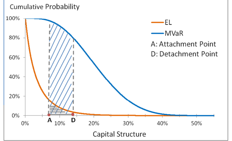
Note: for a discretely thick tranche with attachment and detachment points A and D has EL equal to the area between A and D under the red line, Marginal Value-at-Risk equal to the area under the blue curve between A and D and Unexpected losses equal to the difference between the two. The shape of the EL curve is determined by \\B whereas the shape of the Marginal Value-at-Risk curve is determined by ∗.
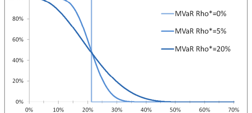
Note: when ∗ is zero, the capital curve is a step function. For higher values, the curve
| Principle | How the Arbitrage | Free Approach | Performs | ||
|---|---|---|---|---|---|
| 1. Objective | The AFA follows | a clear | statistical criterion for risk, | namely that of | |
| statistical | Unexpected Loss. | This is the same | as that employed in Basel | II | for on balance |
| basis | sheet loans. | ||||
| 2. Neutrality | The AFA is capital | neutral. | |||
| 3. Control | The AFA offers a | ∗, parameter, | that may be used by | regulators | to allocate |
| parameters | capital across junior, | mezzanine | and senior tranches in a | smooth | fashion. |
| 4. Transparency | The capital charges | in the | AFA are derived as | simple, | closed form |
| expressions with | no need for | numerical approximation. | The | mathematical | |
| derivation of these | formulae is | transparent, simple and | is | based on well- | |
| known results by | Vasicek, | Gourieroux and Scaillet, | Taasche | (2000) and | |
| Pykhtin and Dev | (2002) and (2003). | The consistency of | the | framework with | |
| the capital charges | for on balance | sheet exposures | substantially | enhances | |
| transparency. | |||||
| 13 | |||||
| The only sense in which | it might have made | sense to adjust | SFA capital at the tranche | level | would have been |
| if the adjustment had | affected the distribution | of capital across | tranches but not the overall | level | of capital. The |
| equivalent of this in the | AFA would be, as | mentioned in an | earlier footnote, possibly allowing | ∗ to depend on | |
| maturity. |
| Kendall's Tau | based | ||||
|---|---|---|---|---|---|
| All regions | All regions | North America | North America | ||
| Sample | 2000-2012 | 2005-2012 | 2000-2012 | 2005-2012 | |
| 1. RMBS | 46.3% | 44.0% | 56.9% | 54.6% | |
| 2. ABS | 30.1% | 28.6% | 32.4% | 30.9% | |
| 3. Other | 20.1% | 18.8% | 29.5% | 28.4% | |
| 4. PF | 23.1% | 22.5% | 23.1% | 22.5% | |
| 5. CDO | 55.3% | 55.5% | 60.9% | 61.1% | |
| 6. CMBS | 35.8% | 36.3% | 38.4% | 39.2% | |
| 7. Structured | Products | 30.4% | 28.9% | 34.8% | 32.9% |
| Maximum | Likelihood based | ||||
| All regions | All regions | North America | North America | ||
| Sample | 2000-2012 | 2005-2012 | 2000-2012 | 2005-2012 | |
| 1. RMBS | 83.9% | 75.1% | 84.2% | 75.2% | |
| 2. ABS | 50.5% | 50.4% | 48.3% | 50.8% | |
| 3. Other | 79.3% | 81.0% | 82.7% | 83.5% | |
| 4. PF | 48.7% | 42.7% | 48.7% | 42.7% | |
| 5. CDO | 68.8% | 77.2% | 76.4% | 85.1% | |
| 6. CMBS | 72.4% | 73.0% | 71.3% | 74.1% | |
| 7. Structured | Products | 65.9% | 64.7% | 84.2% | 75.2% |
| ρ | ρ∗ | ρ∗ | ρ∗ | ρ∗ | |
|---|---|---|---|---|---|
| All | All | North | North | ||
| Assumed | regions | regions | America | America | |
| Basel | 2000- | 2005- | 2000- | 2005- | |
| Sector | value | 2012 | 2012 | 2012 | 2012 |
| 1. RMBS | 15% | 3% | 6% | 3% | 6% |
| 2. ABS | 10% | 11% | 11% | 12% | 11% |
| 3. Other | 10% | 3% | 3% | 2% | 2% |
| 4. PF | 20% | 26% | 34% | 26% | 34% |
| 5. CDO | 20% | 11% | 7% | 8% | 4% |
| 6. CMBS | 9% | 4% | 4% | 4% | 3% |
| 7. Structured Products | 16% | 10% | 10% | 4% | 6% |
References
Ashcraft, Adam and Til Schuermann, (2008) “The Seven Deadly Frictions of Subprime Mortgage Credit Securitisation,” The Investment Professional, Fall, 2-11.
Basel Committee on Bank Supervision (2012) “Revisions to the Basel Securitisation Framework,” Consultative Document, Bank for International Settlements, December.
Basel Committee on Bank Supervision (2013a) “Foundations of the Proposed Modified Supervisory Formula Approach,” Working Paper 22, Bank for International Settlements, January.
Basel Committee on Bank Supervision (2013b) “The Proposed Revised Ratings-Based Approach,” Working Paper 23, Bank for International Settlements, January.
de Servigny, Arnaud and Olivier Renault. (2003) Correlation evidence. Risk, 90-94, July.
Gordy, Michael, (2003) “A Risk-Factor Model Foundation for Ratings-Based Capital Rules.” Journal of Financial Intermediation, 12 (3), 199-232.
Gourieroux, Christian, J. P. Laurent, and Olivier Scaillet (2000) “Sensitivity Analysis of Values at Risk,” Journal of Empirical Finance, 7, 225–245.
Gupton, Greg M., Christopher C. Finger, and Mickey Bhatia (1997) Creditmetrics TechnicalDocument, New York: J.P. Morgan & Co. Incorporated, April.
Heitfield, Erik and Norah Barger (2003) “Treatment of Double-Default and Double-Recovery Effects for Hedged Exposures under Pillar I of the Proposed New Basel Capital Accord,” Federal Reserve Board White Paper, June.
Moody’s (2004) “The Moody’s Capital Model Version 1.0,” International Structured Finance Special Report, January.
Peretyatkin, Vladislav and William Perraudin (2004) “Capital for Structured Products,” Risk Control Limited.
Pykhtin, Michael and Ashish Dev (2002) “Credit Risk in Asset Securitisations: Analytical Model,” Risk, 15(5), S16-S20, May.
Pykhtin, Michael and Ashish Dev (2003) “Credit Risk in Asset Securitisations: The Case of CDOs,” Risk, 16(1), 113-116.
Pykhtin, Michael, (2004) “Asymptotic Model of Economic Capital for Securitisations,” in William Perraudin (ed.), Credit Structured Products, Risk Books.
Tasche, Dirk, (2000) “Conditional Expectation as Quantile Derivative,” November.
Van Landschoot, Astrid and Norbert Jobst (2007) “Rating Migration and Asset Correlation: Structured versus Corporate Portfolios,” in Arnaud de Servigny and Norbert Jobst (eds.) “The Handbook of Structured Finance”, McGraw-Hill.
Appendix 1: Derivation of Expected Losses for Thick Tranches
To derive the expected losses on a senior tranche, we first consider the α-confidence-level Expected
quantile of the loss distribution. Shortfall 0I[2] on the pool of loan losses, i.e., expected losses conditional on losses exceeding the α- ESα (Loss) = E[Loss(Y ) Loss(Y )≥VaRα ]

E[Loss(Y )×1Loss(Y)≥VaRα ]

= P(Loss(Y )≥VaRα )

(A.1.1)

−1 Loss(Y )≥VaRα ⇔ Y ≤ N (α)
−1 −1

N (α) − N (x) ρ + N (p) LGD

notation for the correlation in the underlying pool. where is a generic notation for the probability of default of the underlying pool, and is the generic Let x=N(u) so u=N-1(x).
−1

N (α) LGD −u ρ + N (p)

−1 −1 N (α) ρ LGD N (p) = ∫−∞ N(−au+b)n(u)du; a = &b = α 1− ρ 1− ρ (A1.2)

LGD b −[1] a
![Equation: = N[2] [2] ,N (α),[2] α 1+a 1+a](/api/media/file/eq-21-300x51.png?prefix=media)
LGD −1 −1 = N[2] (N (p), N (α), ρ) α Now, the expected losses on a senior tranche may be expressed in terms of the expected shortfall in
PDTranche(A)× ES(A) − PDTranche(A)× A the following manner, by replacing 3 by ()bdecf: ELSeniorTranche(A) = 1− A LGD PDTranche(A)× × N[2] − PDTranche(A)× A PDTranche(A) = − 1 A LGD× N[2] − PDTranche(A)× A = (A1.3) 1− A
−1 −1 where N[2] ≡ N[2](N (PDPool ), N (PDTranche(A)) , ρ)
![Equation: −[1] −[1] A N ( p) − 1− ρN LGD](/api/media/file/eq-22-300x68.png?prefix=media)
= and PDTranche(A) N

ρ

One may verify that at as the attachment point goes to 0, expected losses go to ( × ,1)) and that as tranche expected losses into the equation for general tranche expected losses gives expected losses for the attachment point goes to the ,1), expected losses go to zero. Plugging the expression for senior a general, discretely thick tranche with attachment point A and detachment point, D.
*
Appendix 2: Methodologies Employed in Estimating ρ
From equations (8) and (9) in the main text, one may deduce the correlation between the risk factors driving the bank’s wider portfolio:
(A2.1) 8& ∗ RmL Z, ≡ L Z, = p To estimate this correlation, we employ two methodologies: (i) the Maximum Likelihood approach developed and applied by Perraudin and Zhou (2012) and (ii) the Kendall’s tau approach applied in Moody’s (2004). Below, for completeness, we provide brief summaries of these methodologies.
The Maximum Likelihood Approach
Suppose there are n = 1,..., N k = 2,1,..., I sectors comprising banks (sector 1) and obligors and several sectors ( 2,..., I ) of different categories of structured product. We will refer to obligors
meaning individual banks or rated securitisation tranches.
Let R(n, t) denote the rating at t of obligor n . Let I (n) be obligor n ’s sector. Suppose that rating
changes at time t for the nth obligor are driven by a Gaussian latent variable:
xn,t = ρn fI(n),t + 1 − ρn εn,t (A2.2)
Here, fI(n),t is the nth obligor’s factor at date t, εn,t is a shock associated with the n th obligor at date
t , and ρn is a constant parameter specific to the nth obligor. We assume that obligors in a given sector have a single common risk factor.
By the usual Ordered Probit argument, the probability that an obligor with rating R(n,t) = i at date t
has a rating j at date t +1equals:
Φ(Zi, j )− Φ(Zi,j−[1]) for j ∈{2,...,J} 1 − Φ(Zi,J−[1] ) for j = J (A2.3)
Φ(Zi1, ) for j = 1
This holds for k = 1,..., J −1 f = 2,1,..., I . and for
In principle, one could seek to estimate correlations ρn using data for all ratings downgrades and upgrades. In this case, for the non-default ratings, 1,...,J −1, one would observe a set of changes in
the rating of each rated obligor over discrete periods of time such as one year.
One may summarize these observations through a (J −1) by J matrix of counts:

Here, N(i, j,t, k) , which is a typical element of the matrix, equals the number of observations for
which the rating goes from i to j for an exposure in sector k between dates t and t +1. If one observes ratings at dates, t = 2,1,0,...,T , one may calculate t = 2,1,...,T such matrices for each of
k = 2,1,..., I sectors.
Now, consider the calculation of the likelihood for ratings changes. If all the ratings changes were independent, we could write the likelihood simply as the product of probabilities of moving from one rating to another taken to powers based on how many observations we have of any given rating change. In fact, ratings changes within a period are dependent. We may proceed by writing down the likelihood conditional on the common factors an then integrate over the common factors.
Given the Ordered Probit formulation, the probability of a rating changing from i to j conditional on a common factor fk,t is:
k k
![Equation: Zi, j − ρk fk,t Zi, j−[1] − ρk fk,t](/api/media/file/eq-26-300x34.png?prefix=media)
Pr (i, j,t, k) = Φ − Φ

1− ρk 1− ρk

for k = 2,1 andt = 2,1,...,T (A2.5)
Plugging these expressions in the product likelihood and integrating over the common factors we get:
∞ T J J N(i, j,t,k) Lk ≡ ∏∫∏∏ Pr(i, j, t, k ) φ( f[1]kt )dfk,t (A2.6) t=2 ∞ i=2 j=2
Note that in writing the above, we omit inconsequential scaling factors (ratios of factorials) which do not affect the value of the correlation parameter that maximizes the likelihood. Also note that the factors are only correlated within a given period, so the integrals appear to the left of the sector and ratings product terms and to the right of the product term with respect to t .
To simplify, instead of modelling all possible ratings changes, one may restrict attention to ratings increases, ratings decreases and observations in which ratings do not change. In this case, one obtains the following likelihood (omitting inconsequential constants):
i−1 N(i,i,k,t) N(i,j,k,t) ∑ ∞ ∞ k k k
![Equation: T J Zi,i−1 − ρk fk,t j=[1] Zi,i − ρk fk,t Zi,i−1 − ρk fk,t Lk ≡ ∏∫∫∏ Φ × Φ − Φ t=[2] −∞−∞ i=[2] 1− ρk 1− ρk 1− ρk](/api/media/file/eq-29-300x29.png?prefix=media)
J N(i,j,k,t) ∑ k
![Equation: Zi,i − ρk fk,t j=i+[1] × 1− Φ φ( fk,t )dfk,t 1− ρk](/api/media/file/eq-30-300x56.png?prefix=media)
(A2.7)
The Kendall’s tau Approach
(DRTM) is calculated. (The concept of a DRTM was devised by Moody’s in a correlation study.) The basic idea of the Kendall’s τ approach is as follows. First, a “directional rating transition matrix”
inferred. Second, from the DRTM, Kendall’s τ is calculated. Third, from Kendall’s τ, the correlation is movements are available, one may record only the direction changes (i.e. ups, no movements, and Assume that there are n cohorts in a sector, and obligors in the cohort i. If the obligors’ rating downs) for each obligor. each element equalling the number of pairs that move in a particular set of directions. Hence, if there For each cohort, a 3 × 3 matrix may be generated (we call it intermediate count matrix here), with
combinations). Summing up the intermediate count matrix for each cohort gives us the total count are obligors in a cohort, the sum of this matrix is × −1 (there are × −1 possible matrix. For each element in this total count matrix, we divide by the sum of all elements and we obtain the intra-sector DRTMs.
Assume that there are a range of sectors and n cohorts in each sector. The procedure to generate the intermediate count matrix is a little different from that employed in obtaining an intra-sector DRTMs. Given any two sectors A and B, suppose there are 5 and obligors in the ith cohorts. Then for the ith cohorts, there are 5 × possible combinations in the intermediate count matrix. Having obtained the intermediate count matrix, as in the intra-sector case, we sum up these intermediate count matrices to obtain the total count matrix, then we divide by the sum of all elements in the total count matrix and thereby obtain a DRTM. The Kendall’s τ measure depends on concordant and discordant pairs and ties among the directional ratings movements. To explain, for any pair of ratings, Y , ; Y, , we say that the pair is
• • Concordant if Y > Y .~6 > , or Y < Y .~6 < ,
• Discordant if Y > Y .~6 < , or Y < Y .~6 > , and A Tie if the pair is neither concordant nor discordant: tie in Y if Y = Y, and tie in if = . For any given sample, Kendall’s τ is defined as: $ $ = $8 $8v $8 $8v (A2.8) Here, R, ), 0, and 0 are the probabilities that a pair is concordant, discordant, or otherwise a tie in Y or in . As the DRTM is 3 × 3 matrix, it contains 9 elements and so 36 possible combinations of pairs must be allocated to concordant, discordant, tie in Y, and tie in . As the DRTM is available, R, ), 0, and 0 can be calculated, then the Kendall’s τ will be obtained.
distributions can be applied to compute the asset correlation between obligors in different sectors. Once Kendall’s τ is determined, a widely used relationship with linear correlation for elliptical Correlation and Kendall’s τ are linked by the following simple equation: : = arcsinρ so that = sinJ : M (A2.9)
Appendix 3: Approximations in the MSFA
1. Introduction
This appendix analyses approximations employed in the tranche capital charge calculations in the Basel MSFA paper. This appendix uses the same notation as in the Basel MSFA paper. The primary approximation of the MSFA is to replace the distribution of losses, slightly transformed and adjusted, with the cumulative distribution function of a beta-distributed random variable.
The beta distribution is then parameterised by calculating a mean and variance of future loan losses in a two period model (with the historical loss distribution used in the first period and the risk adjusted distribution employed in the second period) and then plugging this into the beta distribution. The mean and variance are not calculated exactly but, instead, are replaced with approximations.
Evaluating the approximations used in the MSFA is complicated by an error in the published Basel document which is apparently not present in the actual approximation calculations. Having corrected this error, we have confirmed the calculations reported in the Basel document on the accuracy of the mean approximation. Our analysis of the accuracy of the variance approximation suggests that the true value of the variance is, for safer tranches, half as large as the approximation. For riskier tranches, the degree of conservatism is less but the approximated variance is always greater than the true value. Some of the arguments made to justify the approximations appear to us to be tenuous.
Section 3.2 of the appendix describes the use of the beta distribution approximation. Sections 3.3 and 3.4 discuss approximations used in benchmarking, respectively, the mean and variances of losses.
2. Approximating the Distribution of Losses with a Beta Distribution
Consider a tranche with notional attachment and detachment points A and D, the tranche’s ES-based capital charge is given by the paper’s equation (7):
In the MSFA, tranche capital charges are calibrated assuming that the tranche coupon rate RT=R. This implies the paper’s equation (8):
' K [z] The paper defines F[z] ≡ 1− ' . Over the range [0,1], F[z] has the properties of a CDF. K[z] can K [0]
be approximated by replacing it with a convenient distribution function. Suppose that B[z;γ,δ] is a
beta distribution with parameters γ and δ. Then suppose as is done in the paper’s equation (11) that:
Here, if Fˆ[z] ≡ B[z;γ,δ] is the CDF for a beta distribution with parameters γand, then the mean
and variance of the beta distribution equal µand σ .
The capital charge in (8) is then approximated as I the paper’s equation (13):
The rest of this note describes the approximations employed in calibrating the EGˆ , VG ˆ parameters. In
future work, we will evaluate hG ˆ and the use of the beta approximation overall.
3. Approximations Employed in the Calculation of Mean Losses EGˆ
The pool’s expected loss rate (at t=0) under the conditional probability distribution implied by the regulatory model is expressed by the paper’s equation (25):
In the above equation defining W, DTM* should be pre-multiplied by M . The approximations performed in the MSFA paper appear to have been done using the correct expressions rather than
terms omitting M . The above expression for wj is approximated with a simpler function given in
the paper’s equation (26):
Figure A3.1: Comparison between integration from (25) and approximation from (26)
Comparioson between approximated and integrated values of w 0.9
45-degrees Approximation vs. Integration 0.8
0.7
0.6
0.5
0.4 Integration
0.3
0.2
0.1
0 0.1 0.2 0.3 0.4 0.5 0.6 0.7 0.8 0.9 Approximation
Figure A3.1 summarises the quality of this approximation over a broad parameter range: M= {2, 3, 4, 5}, AVC={0.05, 0.15, 0.25}^2 and PD1=0.03% ~ 30%. All the points lie close to the 45 degree line.
The EGˆ is estimated by using estimator wˆ j , i.e., as in the paper’s equation (27):
Clearly, the approximation in (26) is accurate.
4. Approximations Employed in the Calculation of the Variance of Losses VG ˆ
The regulatory model’s implied conditional risk-neutral variance for pool credit losses is expressed by the paper’s equation (28):
Here,
In the MSFA paper, the last term in (28) is bounded as in the paper’s equation (30):
From (28) and (30), one may obtain the paper’s equation (31):
The next approximation consists of replacing Covii with an upper bound deduced from a few
calculations of particular cases. The upper bound is stated in the paper’s equation (32):
The final result after all these approximations is given in the paper’s equation (33):
where
In Figure 2, the values of wi used in (28) is from (25) by integration and in (33) is approximated by (26).
The claimed upper bound in the second line of the paper’s equation (30) holds only if the COVii and COVjj terms are as described in the paper equal to the variances of the individual default indicators for the ith and jth obligors. The approximation reported in the paper instead appears to be based on the pairwise correlations of pairs of exposures with the parameters of a given exposure such as i. While this is an intermediate step and hence does not invalidate the final approximation, it means the description of how the approximation is derived inconsistent with what has actually been done.
Figures 2 summarises the quality of the approximations made in calibrating VG ˆ . The assumptions made are as follows: PD1: 0~10%, M={2,3,4,5}, qES = 0.003, LGD = 0.5 and N = 100 loans in the pool. AVC is the IRB framework’s implied correlation and is expressed by:
AVC=0.12*(1-exp(-50*PD1))+0.24*exp(-50*PD1)
Figure A3.2: Comparison between actual values from (28) and approximations from (33)
-3 Actual and Approximation Values of Vg 6 x 10
45-degrees Approximation vs. Actual
Actual
0 1 2 3 4 5 6 -3 Approximation x 10
As may be observed from Figure A3.2, the variance approximation is very conservative. The true variance is always less than the approximation, sometimes for safer deals being half the size.
Appendix 4: Step-by-Step Implementation of the AFA (Option 2)
With the following IRBA inputs for each asset
1. the one-year probability of default ()
2. the loss given default ,1)
3. the systemic correlation (defined in BCBS128)
4. the exposure at default 05) &89 :.< ∙=>.&&?<: >.><@A?∙B CD & &.<∙=>.&&?<: >.><@A?∙B CD ' with the asset
5. the Maturity Adjustment as *.4567 = exposures, including mortgages. maturity * for corporates, sovereigns and bank exposures. *.4567 = 1 for retail ∗, set by national regulators for their respective national asset class, to be applied in all Basel-regulated jurisdictions (to avoid arbitrage), and given a the new ‘stressed’ correlation depending on the type of securitisation:
Calculate for the asset, the asset dependent value:
• the maturity-adjusted probability of default: ()′ = () ∙ *.4567
• the maturity-adjusted stressed probability of default: &() + ∙ &99.9% l ∙*.4567 I()′ = g 1 − standard normal distribution; is the inverse of the Here, is the standard normal distribution and where &
• the unexpected loss contribution to Bank of the asset: %XST = I()′ ∙ ,1) − ()′ ∙ ,1) Calculate for each asset, the pool-dependent values:
• the weight t of an asset u in a pool, with a pool size 05) \\B. 05) t = 05) \\B
• the granularity adjustment[18] of asset u is given by the consolidated weight of all assets belonging to the same obligor as the obligor of asset u in the pool: = t , ⊂e Calculate for each tranche, the tranche-dependent and asset-dependent values: For the tranche | with the effective attachment point of the tranche 5, and the effective detachment point of the tranche ), the contribution of an asset u to the tranche need the following intermediary steps for a theoretical (mm :
• the pool correlation ]^^_ in a theoretical pool (mm , made of homogeneous assets sharing the same characteristics as asset u is given by: ∗
![Equation: ]^^_ = + 1 − ∙](/api/media/file/eq-31-300x135.png?prefix=media)
• the Vasicek granularity adjusted pool correlation:
![Equation: ′ ]^^_ = ]^^_ + ∙ J1 − ]^^_M](/api/media/file/eq-32-300x99.png?prefix=media)
• the Vasicek granularity adjusted stressed correlation: ∗ ∗ + ∙ 1 − ′ ]^^_ =
• the Probability of Default of the tranche ()b, 5 : ()b, 5 = -.uG ()b J5, ()′ , ,1) , ′ ]^^_M
• the Loss Given Default of the tranche ,1)b, 5, ) : ,1)b, 5, ) = -.uG ,1)b J5, ), ()b, 5 , ()b, ) , ()′ , ,1) , ′ ]^^_M
• the Stressed PD of the tranche I()b, 5 is given by: I()b, 5 = -.uG ()b J5, I()′ , ,1) , ′ ]^^_M
• the Stressed LGD of the tranche I,1)b, 5, ) : I,1)b, 5, ) = -.uG ,1)b J5, ), I()b, 5 , I()b, ) , I()′ , ,1) , ′ ]^^_M
at Risk of the Bank, at the financial stability confidence level (FSCL=99.9%):
• the contribution of asset u to the Marginal Contribution of the tranche | to the Value %*Rb, -./,L¡ = t ∙ I()b, ∙ I,1)b,
Expected Loss of the Bank:
• the contribution of asset u to the Marginal Contribution of the tranche | to the %*Rb, 0, = t ∙ ()b, ∙ ,1)b,
Risk Charge of the Bank:
• the contribution of asset u to the Marginal Contribution of the tranche | to the Model %*Rb, */R = t ∙ =6% ∙%XSTC Aggregate for each tranche, the contributions to the marginal contributions: ¢¢f£¢ %*Rb, -./,L¡ %*Rb-./,L¡ = ¤& ¢¢f£¢ %*Rb, 0, %*Rb0, = ¤& ¢¢f£¢ %*Rb, */R %*Rb*/R = ¤&
Apply the Basel II formula for the 3 Unexpected Loss Components: %R/ST¥ = %*Rb-./,L¡ −%*Rb0, + %*Rb*/R Multiply by the thickness to move from percentage notation (applied to the tranche’s notional) to ‘dollar’ notation (applied to the pool’s notional): $R/ST¥ = $)b −$5b ∙ %R/§/| *** *** b should be equal to $R/ST]^^_. Final coherence check (prior to adjustments): ∑ $R/§/|
given below: The function -.uG ()b5, , n6, and -.uG ,1)b5, ), b5 , b) , , n6, are -.uG ()b5, , n6, ¬ u 5 ≥n6, 4ℎG~ b5 = 0% ª & − 1 − ∙ & 5 n6' = u 0 < 5 < n6, 4ℎG~ b5 = ¯ ° « ª ©u 5 = 0, 4ℎG~ b5 = 100% -.uG ,1)b5, ), b5 , b) , , n6, ¬u 5 ≥n6, 4ℎG~ n6b = 0% b) = n6 b5 ∙ ) −5 « u 0 ≤5 < n6, 4ℎG~ n6b = + l ) −5 ) −5 ∙ g-, b5 , −-, b5 b) , © where -, bY , u Y ≥n6, 4ℎG~ -, bY , = 0% = ±u 0 < Y < n6, 4ℎG~ -, bY , = := & , &=bY C, C u Y = 0, 4ℎG~ -, bY , = with :{, ², } being the bivariate cumulative standard normal distribution function[19].
19 The : function is easily implementable in Excel using VBA.
Notes
[1] Dr. Georges Duponcheele is Head of Banking Solutions Private Side, BNP Paribas. Dr. Daniel Totouom-Tangho is in Credit Quantitative Research, BNP Paribas. William Perraudin is a Director of RCL and Adjunct Professor of Imperial College, London. Correspondence should be addressed to the authors at georges.duponcheele@bnpparibas.com, daniel.totouom-tangho@bnpparibas.com or william.perraudin@riskcontrollimited.com.
[2] The authors thank Fabrice Susini, Laurent Carlier, Antoine Chausson, Duc Dam Hieu, Alexandre Linden, Eric Silie, Iuliana Dincov, Vincent Mayot, Christopher Morgan and Jean Saglio for their contribution, their numerous and helpful comments. Duponcheele and Totouom-Tangho thank Manish Chandra and Kaiwen Xu for ensuring that time was made available to develop this solution. Additional discussions with Alexander Batchvarov, Shalom Benaim, Vivien Brunel, Norbert Jobst and Alastair Pickett have also been welcome. All errors are ours. The views expressed are the authors’ own and not necessarily those of BNP Paribas nor those with whom we had discussions or their firms.
[3] Arguments can be made that the involvement of multiple agents in securitisation may generate agency problems. Ashcraft and Schuermann (2008) discusses conflicts of interest in securitisation processes and attributes the sub-prime crisis in part to such agency problems. In our view, if securitisations are properly evaluated by ratings agencies and auditors and if originators retain some “skin in the game”, agency problems should not add substantial additional risk. When little data is available on the historical performance of underlying assets, there may be additional risk. This issue certainly contributed to the problems experienced with US sub-prime mortgages in that ratings agencies had little information on which to base criteria. Note that lack of data and historical experience affects the risk of on-balance-sheet lending as well as that of securitisations.
[4] Note that the Pykhtin-Dev model was previously used in the calibration of the Ratings Based Approach (RBA) to securitisation capital in Basel II. The calculations performed for that purpose are reported in Peretyaktin and Perraudin (2004). The calibration was performed so as to ensure that, allowing for supervisory over-rides, when all the tranches in a structure were rated and capital was calculated using the RBA, the implied capital for a bank holding all the tranches was similar to that required for holding the underlying assets on balance sheet. In this sense, the RBA calibration was capital neutral and did not aim to give credit for diversification, contrary to statements in BCBS (2013b).
[5] The so-called Asymptotic Single Risk Factor Model (ASRFM) exposited in Gordy (2003) and described in BCBS (2005) focusses on default risk over a one-year horizon. Risk associated with rating transitions that occur before the end of the year are not directly modelled but instead are handled, for corporate exposures at least, through a maturity adjustment. This approach was taken not because the Basel authorities believed transition risk should be ignored but because developing explicit formulae based on a more elaborate model was viewed as infeasible. Formulae based on the default mode ASRFM with a maturity adjustment were employed as convenient functional forms that could be fitted by adjusting correlation parameters to capital levels that had been separately calculated using Monte Carlo and other multi-period models that included transition risk.
[6] One might question whether asset level and tranche level maturity adjustments are required. Certainly, tranche level adjustments should not affect the aggregate capital for all tranches together. Agency problems aside, securitisation reallocates risk but does not change the total level of risk that is appropriate to the structure as a whole. There may be a case for allowing the distribution of capital across tranches to depend on maturity. determines the allocation of capital across seniority levels) to depend on maturity. We intend to examine the Within our framework as described below, this would correspond to allowing the ∗parameter (which scope for this in future work. 2. Neutrality The MSFA turns fundamentally away from the notion of neutrality in that the securitisation capital it implies would be completely different from on balance sheet IRB capital charges. The primary difference it introduces is a very complex and substantially over-engineered mark-to-market adjustment. The effect is substantial and the approximations rough, requiring the introduction of an ‘overall cap’ and a ‘risk-weight cap’ to ensure that the capital on a senior position does not exceed the total capital on an underlying pool. The MSFA like the SFA includes a ‘tau’ parameter designed to create a 3. Control smooth ‘S-shape’ curve that distributes capital across tranches of different parameters seniorities. The parameter has no economic sense, however, and as far as we are aware, no evidence has ever been presented to motivate different values. 4. Transparency The multiple layers of approximation and the fundamental differences between the assumptions adopted in the MSFA and those employed elsewhere in the capital framework substantially reduce the transparency of the Basel capital regulations. distribution function.
[8] For corporate, sovereign and bank exposures, the correlation is dependent on the probability of default with = 12% ∙ 1 −G <>∙ + 24% ∙G <>∙ and for SME, there is another adjustment to the correlation based on the size of the firm Sales €L €< I (in €million), where the correlation is adjusted downwards with the term For retail exposures, the correlation is dependent on asset type: 4% ∙ J1 − €@< M (with I floored at €5 million and capped at €50 million). • • for residential mortgage exposures: = = 15% • for revolving retail exposures: = = 4% for other retail exposures: = 3% ∙ 1 −G P<∙ + 16% ∙G P<∙ ∗ ^' ≤ &()\ \ = − \ + 1 −\ \o∗ Y\o + p1 −\o ∗ r' ≤ &=()oC o = − o + p1 −o \o∗ Y\o + p1 −\o the guarantor. The model contains three correlation parameters, the systematic correlations of the obligor and In this two factor model, affects all exposures in the bank’s portfolio while Y\o only affects the obligor and ∗ p1 −\ =1 −oC, the obligor-guarantor asset correlation. guarantor, \, o, and \o = \ o + \o ∗ greater than zero, represents the fact that the obligor and guarantor may be exposed to common shocks over and beyond those associated with systemic risk. Having \o
[10] By ‘homogeneous’, we mean here that PD, LGD and systemic correlation parameter are all equal for different exposures.
[11] The bivariate, Gaussian cumulative distributions function, N[2], is easily implementable in Excel using VBA.
[12] For example, in S&P CLO methodology for corporates, the intra-sector correlation is 20%, whereas the inter- sector correlation is 7.5%. This illustrates the point that correlations are higher for concentrated pools than for for a set of securitisations and then comparing these with estimates of individual bank portfolio correlation estimates. This approach is demanding in data. We intend to explore such an approach in future work.
[15] In other work, we have examined the performance of the estimator here employed through Monte Carlo analysis and found it to be reliable. Details are available on request from the authors. estimates for L, are biased down with the result that the implied ∗ are biased up.
[17] No set of capital formulae including the one we present here can solve all problems, and there will always be features of specific deals (including, for example, non-credit-related, additional risks) that are not addressed in a wholly satisfactory way. As long as these cases are genuinely exceptional and add little to the balance sheet risk of a large and diversified bank, then the approach remains viable.
[18] This granularity adjustment is valid only for Option 2 of Section 5. Another formula applies for Option 1.