

Rating transition matrices for sovereigns are an important input to risk management of portfolios of emerging market credit exposures. They are widely used both in credit portfolio management and to calculate future loss distributions for pricing purposes. However, few sovereigns and almost no low credit quality sovereigns have ratings histories longer than a decade, so estimating such matrices is difficult. This paper shows how one may combine information from sovereign defaults observed over a longer period and a broader set of countries to derive estimates of sovereign transition matrices. * Birkbeck College, yhu@econ.bbk.ac.uk ** London School of Economics, r.t.kiesel@lse.ac.uk *** Birkbeck College, Bank of England and CEPR, wperraudin@econ.bbk.ac.uk The authors thank Paul Radford, John Waterman and other ECGD staff, and an anonymous referee for extremely helpful comments. Views expressed are those of the authors and not necessarily those of the Bank of England.
Research Paper
The Estimation of Transition Matrices for Sovereign Credit Ratings
Date:2002 Reference Number:2/2
The Estimation of Transition Matrices for Sovereign Credit Ratings
Yen-Ting Hu*, Rudiger Kiesel** and William Perraudin***
January 2002
1.Introduction
Transition probabilities between different credit ratings play a crucial role in any ratingbased credit portfolio model. The difficulty faced by analysts wishing to estimate such probabilities for particular types of obligor, however, is the lack of data. If one is prepared to assume that the same transition probabilities hold for any type of obligor, then one may employ the substantial data sets of ratings histories published by the two primary rating agencies, Moody’s and Standard and Poor’s. The Moody’s dataset, for example, includes approximately 60,000 yearly ratings observations if one pools the data for all the individual obligors covered by Moody’s since 1970.
However, the Moody’s data, like that of Standard and Poor’s, is heavily weighted, in the pre-1990 period, towards US industrials. Post-1990, the agencies have rated large numbers of obligors from other countries, but the majority of these have been banks or financials. If one’s primary interest is in a specific group of obligors (examples might be European industrials or emerging market sovereigns), the number of annual observations of rating transitions available is quite small. The problem is particularly great if one wishes to estimate transition probabilities for low credit quality issuers in such specific categories since, outside the US, rating agencies primarily rate high credit quality issuers.
This paper shows how one may estimate transition probabilities for an important class of obligors, namely sovereign issuers. Sovereign transition matrices are widely used in credit portfolio modelling and in calculating future loss distributions for pricing purposes. The techniques we develop allow one to combine the relatively small amount of transition data available for sovereigns with information on sovereign defaults for a broader set of countries and over a longer period of time.
More precisely, our approach consists of modelling sovereign defaults and Standard and Poor’s sovereign ratings within a common Maximum Likelihood, ordered probit framework. The credit standing of any given obligor in a given year is assumed to be governed by a latent variable consisting of a random error plus an index, Xβ, of current and lagged macroeconomic variables including measures of indebtedness.
When no rating is available, the likelihood for a given sovereign is based on whether that sovereign is in default or not. When a rating is available, the likelihood consists of the probability that the sovereign is in the rating category observed. Use of this common framework enables us to pool information from rated and non-rated sovereigns in different years.
Having estimated our model, we employ it to predict which rating category each obligor would have occupied for each year of our sample. Using the “fitted” rating histories generated in this way, we estimate rating transition matrices. The number of observations of forecast rating transitions is considerably greater than the number of observations of actual rating transitions, and it is in this sense that our approach adds information to what one could achieve using naive estimators of sovereign transition probabilities.
The last topic we examine is how one may apply Bayesian techniques to combine the sovereign transition matrix estimates with the additional information supplied by transition matrices estimated from larger samples such as industrial obligors. The approach we describe is based on methods proposed in a different context, namely the Bayesian estimation of contingency tables. Effectively, our approach consists of taking weighted averages of transition matrix estimates obtained in different ways, where the weights are selected in a data-driven way based on a goodness of fit statistic.
One may compare the techniques developed in this article with other recent work on estimation of rating transition matrices with few observations. Lando and Skodeberg apply continuous-time methods to estimate transition matrices. They effectively make use of the additional information provided by the time a given obligor spends in a given rating category. Within this framework, they show how one may estimate the transition intensities for the (possible non-homogeneous) Markov chain and calculate the corresponding discrete-time transition matrix. Typically, these matrices have non-zero one-year transition probabilities even for rare events such as a transition from the highest rating category to default. The Bayesian methods we describe above have a similar effect in that they tend to lead to a spread of probability weight into states that would otherwise have zero transition probabilities.
The structure of the paper is as follows. Section 2 discusses the ordered probit framework within which we model both sovereign ratings and defaults. Section 3 provides information about our data set and examines which macroeconomic variables should sensibly be included in a model of sovereign credit standing. Section 4 sets out the probit estimation results. Section 5 discusses the transition probabilities they imply. Section 6 introduces some Bayesian techniques for combining different transition matrix estimates. Section 7 evaluates the ratings and default predictions produced by the model by examining how many sovereigns are correctly and incorrectly classified in different years on an in-sample and a leave-one-year-out basis. Section 8 concludes.
2. An Ordered Probit for Ratings and Defaults
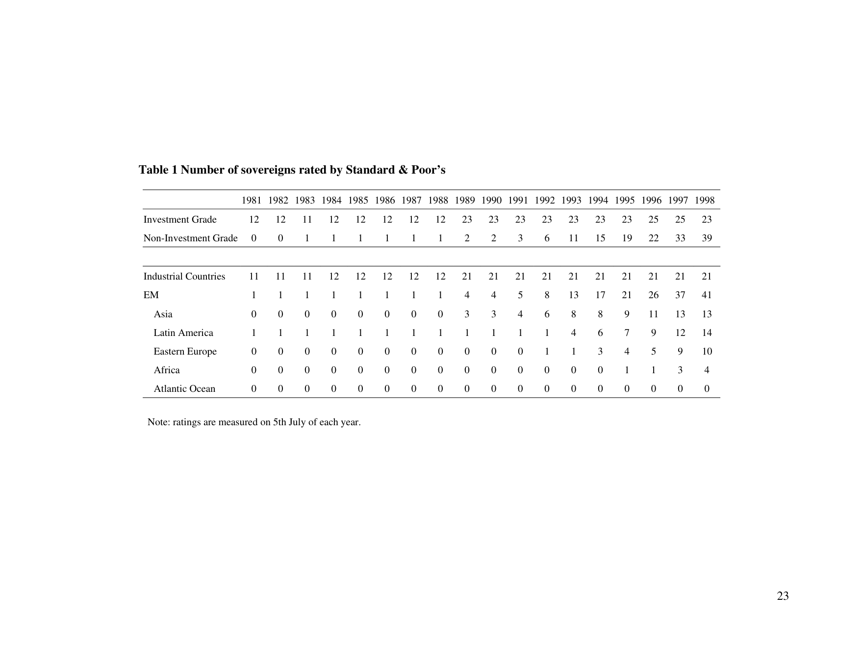
The basic problem in estimating transition matrices for sovereigns is the relative lack of available data. Table 1 shows the numbers of sovereigns from different geographical areas and credit qualities that were rated by Standard and Poor’s at various dates since
1981. The table demonstrates that the number of rated sovereigns has grown substantially over the last decade, with increases particularly in the numbers of Asian, Latin American and Eastern European sovereigns that have ratings. But, very few sovereigns have long rating histories. In 1990, only 26 sovereigns were rated of which only 5 were non-industrial countries.
But estimating transition matrices requires large numbers of observations of rating transitions. Even a rating matrix for the coarse rating categories, AAA, AA, A, BBB, BB, B, CCC and default contains 49 elements that require estimation. If one is interested in finer rating categories, the number of elements to estimate is very considerable. For example, if one takes AAA, AA, A, BBB+, BBB, BBB-, BB+, BB, BB-, B+, B, B-, CCC and default, the number of unconstrained elements to be estimated is 169.
It is true that many of the more off-diagonal elements are likely to equal zero. But, even if the matrix has no more than four non-zero elements in each row, 39 entries must be estimated. In the period 1981 to 1998, the number of annual observations of Standard and Poor’s sovereigns ratings[1] is 487 of which only 158 have ratings below single A. The number of annual observations of changes in ratings is 26 of which just 13 are changes for which the initial rating was below single A.
It is therefore important to find ways of introducing other kinds of information to improve the transition probability estimates. Several approaches may be taken. An obvious approach might be to suppose that the rating transition matrix for other, nonsovereign obligors resembles that for sovereigns and to take a weighted average of estimates of both. Although this would have the advantage of simplicity, we feel there is too much evidence that sovereign and non-sovereign ratings behave differently to justify this approach.
Jackson and Perraudin (2000) point out that, on average, credit spreads for sovereigns are distinctly lower than those of corporates with the same rating. Cantor and Packer
(1996) show that rating agencies disagree about sovereign ratings more than they do about corporates. Perhaps most pertinently, Nickell, Perraudin and Varotto (2000) show that sovereign rating transitions matrices differ significantly from those of US industrials.
We therefore prefer to supplement the information contained in available data on rated sovereigns with information about sovereign defaults. The Export Credit Guarantee Department (ECGD) of the UK government supplied us with data on defaults by a broad set of countries. We provide more detail about this data in Section 3 but, in brief, using it we are able to increase the number of observations in our sample substantially to 1069, thereby substantially increasing the amount of information available to us in estimating transition matrices.[2]
The framework we employ to pool information on sovereign ratings and defaults is an ordered probit model. The basic assumption of this approach is that credit standing is driven by an index of relevant predetermined variables such as debt ratios and inflation, plus a normally distributed random error. The model we estimate resembles that of Nickell, Perraudin and Varotto (2000).[3]
The assumptions of the ordered probit model may be stated formally as follows (for more details, see Green (1997), §19.8). Suppose there are J+1 rating categories and the initial rating of a particular obligor is i. The terminal rating at the end of one period, j, is determined by the realization of a latent variable, R, in that j = 0 if R ≤ 0 ⎧ j = 1 if0 < R ≤ Z ⎪[2] (1) ⎨ M M ⎪ ⎪⎩ j = J +1 if ZJ ≤ R where the Zk are scalar cut-off points. It is assumed that R = β' X +ε where X is a vector of predetermined variables, β is a vector of parameters and ε is assumed to have a standard normal distribution.
Statistical implementation of this model involves the estimation of the vector of cut-off points Z and of the vector of parameters β. The probabilities of being in each category are Prob( j = 0) = Φ −β' X ⎧ ( ) Prob( j = )1 = Φ(Z −β' X ) ⎪[1] (2) ⎨ = M M ⎪ ⎪⎩Prob( j = J +)1=1− Φ(ZJ −β' X ) where 0 < Z[1]<…< ZJ. Given these expressions for probabilities and data on the future ratings of a set of obligors with an initial rating i, one may estimate the model using maximum likelihood techniques.
For many sovereigns and time periods, agency ratings are not available, however, but it is known whether or not the sovereign defaulted in given years. In this case, one may still form a likelihood for the observation in question by including the conditional probability that default does or does not occur, i.e., Φ − β' X ⎧Prob( j = 0) = ( ) (3) ⎨ Prob( j > 0) =1− Φ(− β' X ) ⎩ By combining likelihood entries of the kind shown in equation (2) (for cases in which ratings are observed) with likelihood entries of the type shown in equation (3) (for cases in which ratings are not observed but it is known whether default took place), we are able to include many more countries and time periods than if we estimated the model solely using observations for which we have ratings. One way to characterize this approach is to regard the default/non-default observations as helping to pin down the β parameters, while the observations for which we have ratings help to determine the cut-off points between the rating categories (while also conveying information about the β’s).
Once estimates of the model parameters, the Z’s and the β’s, have been obtained, one may predict the rating for each sovereign and each year in the sample by calculating the index β' Xkt (where k indicates a particular sovereign and t the time period) and noting the range [Zj-1,Zj] into which it falls. By this approach one may create rating histories for all the countries in the sample covering the entire sample period. The rating histories may be used to estimate rating transition matrices just as one might estimate a transition matrix using actual observed rating histories, by calculating the fraction of sovereigns initially rated i that moved to rating j within the course of one period. The final step is to take a weighted average of the rating transition matrix based on probit estimations and a naïve estimate of the rating transition matrix based simply on relative frequencies of transitions.
3. The Data Employed
Throughout our analysis, we use Standard and Poor’s ratings observed on 5th July of each year. The results would probably be similar if we used Moody’s ratings. Cantor and Packer (1996) note that of the 49 sovereigns rated by both Moody’s and Standard and Poor’s in September 1995, 28 had the same rating. Of those with different ratings, the discrepancy was just one notch (e.g., AA- instead of Aa2) for all except 7 cases in which the ratings were two notches apart.
The numbers of annual observations of sovereigns in different rating categories is shown in Figure 1. As noted above, there are 487 annual observations of Standard and Poor’s sovereign ratings of which only 158 have ratings below single A. The main points that emerge from the figure are:
• There are a large number of observations of high credit quality sovereigns, reflecting the presence in the sample of industrial country sovereigns.
• Sovereigns in the middle of the B-range are well-represented but the high BBB’s and low B’s included in the sample are very few. There are almost no CCC’s. It is apparent from this that, in estimating the model, it will prove difficult to distinguish the BBB+/A cut-off point and that the boundaries between B, B- and CCC categories will be difficult to pin down.
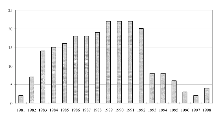
For periods in which ratings data is not available for a given sovereign, we use default data provided by the ECGD. Few countries have ever defaulted on public bond issues and hence ratings histories contain almost no observations of defaults. But, especially in the 1980s, many countries defaulted on their bank debt and trade credit obligations. Figure 2 shows the evolution of the number of defaults over time. It is notable that the debt crisis of the early 1980s persisted right through until the early 1990s and that only in 1993 was there a major reduction in defaults.
The explanatory variables in our model are variables that one might reasonably expect would influence credit standing. Regressors are included with no lags.[4] To deduce which variables to include, we draw on several past empirical studies. These studies have examined determinants (i) of sovereign ratings (see Cantor and Packer (1996), Haque, Kumar, Mark and Mathieson (1996), Juttner and McCarthy (1998), Monfort and Mulder (2000)), (ii) of sovereign defaults (see Edwards (1984)), and (iii) of spreads on sovereign debt (see Burton and Inoue (1985), Edwards (1986), Cantor and Packer (1996), Eichengreen and Mody (1998), Min (1998), Kamin and Kleist (1999)).
The variables commonly used in past studies of sovereign credit standing may be classified in to
1. Liquidity variables. These variables include components of balance of payments that reflect a country’s short-run financing problems. Typically, they are in the form of ratios that proxy capital in- and outflows. The most important examples are (i) the debt-service-to-export ratio, (ii) the interest-service ratio (i.e., the ratio of interest payments to exports during a given period), and (iii) the liquidity gap ratio (i.e., one-year short-term debt minus current account balance as a ratio to available funding (capital inflows). Most empirical studies have found the debt-service-to-export indicator to be the most significant of the above indicators.
2. Solvency variables. These are related to the liquidity variables in that they are intended to measure for a country’s medium to long-term ability to service its debt. Examples include: (i) the reserves-to-imports ratio, (ii) export fluctuations (usually expressed as export growth as a deviation from trend), (iii) the debt to GDP ratio.
3. Macroeconomic fundamentals. These variables reflect a county’s long-run prospects and are used to assess the quality of a country’s government and the economic dynamics within an economy. Examples include: (i) the inflation rate,
(ii) the real exchange rate, (iii) the GDP growth rate, (iv) the growth rate of exports.
4. External Shocks. Variables of this kind include: (i) changes in US Treasury interest rates (ii) changes in the real oil price.
In our choice of variables, we are most influenced by the studies of Cantor and Packer
(1996) and Monfort and Mulder (2000). Cantor and Packer (1996) show that per capita income, inflation, external debt, an indicator of economic development and an indicator of default history all have significant coefficients in a regression of ratings (expressed as a numerical index) on a range of macro variables. Their regression explains 90% of the variation in the ratings of 49 countries observed in 1995.
Monfort and Mulder (2000) estimate an error correction model for ratings that permits short-run behaviour to differ from long-run relations. They argue this is consistent with the expressed policy of ratings agencies of rating through the cycle. In their long-run ratings regressions, Monfort and Mulder (2000) find all those suggested by Cantor and Packer (1996) are significant except for per capita income. In addition, current account/GDP is very significant although it has the wrong sign. Variables suggested by Edwards (1984) (investment/GDP) and by Haque, Kumar, Mark and Mathieson (1996) (terms of trade and export growth rate) are also significant.
The variables we included in the most general models we estimated were:
1. A dummy variable for past default during the sample period.
2. A dummy variable for default in the previous year.
3. Regional dummies.
4. The ratio of debt service to exports.
5. The debt to GNP ratio.
6. The ratio of reserves to total foreign debt.
7. The ratio of reserves to imports.
8. The rate of consumer price inflation.
9. The rate of GNP growth.
10. A dummy for non-industrial countries.
We were reluctant to include external shock variables since, given the twenty-year length of the sample period, time series variables tend to pick up trends or to act as time dummies. In effect, they serve to describe the sample rather than to help in forecasting. The variables we list seem to us a selection of the most promising liquidity and solvency variables and macro-factors. We focused on these variables also because they were all available for large numbers of countries in a consistent form on World Bank and IMF data CDs. Our sample period of 1981 to 1998 was dictated partly by the availability of this data but more importantly by the period over which we could obtain default data from the ECGD.
As well as providing guidance on the selection of explanatory variables, past studies have implications for the dynamic specification of the model. Juttner and McCarthy
(1998) argue that the findings of Cantor and Packer (1996) are not stable if one repeats their regression including subsequent years. The crisis year of 1998 appears to depart from the relationships found by Cantor and Packer (1996) substantially. Monfort and Mulder (2000) find that the relationship they estimate is not stable if one splits the sample. Variables that remain significant for all three of the sub-samples they consider are debt/exports, rescheduling, the fiscal balance, output growth and inflation. The R[2]’s estimated by Monfort and Mulder (2000) for Moody’s and Standard and Poor’s ratings are mostly lower than the 90% found by Cantor and Packer (1996) and decline at the end of the sample to 50%.
Monfort and Mulder (2000) stress that misclassifications of countries into different rating category by static models of the kind estimated by Cantor and Packer (1996) are serially correlated. One technique for dealing with this is to introduce lagged ratings as explanatory variables and this is the approach followed by Monfort and Mulder (2000). In our case, since we wished to generate predicted ratings running back in time to the start of our sample period for countries lacking agency ratings, this approach was difficult to implement. We therefore instead allowed for richer dynamics in the explanatory variables by including them lagged once as well as with no lag.
4. Default Model Estimation Results
We estimated models with the regressors listed in the last section included both as contemporaneous and lagged variables. We then reduced the number of variables to those that were highly statistically significant. The selection criterion we applied in variable selection was to drop variables successively that had t-statistics with absolute values significantly less than 2. We do not report the results of our intermediate estimations because of space constraints.
Table 2 contains results for our preferred two models. The first model, referred to as the coarse rating model, includes eight ratings categories, namely AAA, AA, A, BBB, BB, B, CCC, and default. The second model, denoted the fine rating model, includes the rating categories AAA, AA, A, BBB+, BBB, BBB-, BB+, BB, BB-, B+, B, B-, CCC, and default. The explanatory variables included in both the coarse and fine rating models as well as a constant are:
1. A dummy variable equal to unity if the sovereign has defaulted in the previous year
2. The ratio of Debt to GNP.
3. The ratio of foreign exchange reserves to total imports
4. The rate of consumer price inflation.
5. A dummy which equals unity if the sovereign is a non-industrial country and zero otherwise.
6. The lagged ratio of debt service to export.
7. Lagged consumer price inflation. The signs of the parameters are generally as expected. Past default, lower reserves, higher inflation, a higher debt to GNP ratio, being a non-industrial country and a higher ratio of debt service to exports all contribute to lower current credit quality. All variables have coefficients that are significant at conventional confidence levels.
It is noticeable in the results reported in Table 2 that the parameter estimates for the fine rating model closely resemble those for the coarse rating model. This reflects the fact that the default/no default observations play the larger role in pinning down the estimates of the β’s.
The cut-off parameters shown in Table 2 represent the square root of the gap between successive cut-off points. (They are squared within the estimation algorithm to preserve the positivity of the gap between successive cut-offs.) Since we include a constant among the independent variables, we normalize the first cut-off point to zero. Of the cut-off parameter estimates reported in the table, the most problematical are the first in the coarse rating model and the first two in the fine rating model. These correspond to the square root of the width of the CCC range in both models and to the square root of the width of the B- range in the fine rating model. The estimation is hampered by the fact that there is only a single observation of a Standard and Poor’s CCC rating in the sample and similarly only a single B- observation. The result is that the gaps between the estimated cut-off points in the sample around CCC and B poorly estimated, being extremely small.
5. Rating Transition Probabilities
Having estimated the parameters of the coarse and fine ratings models, we are able to generate predicted ratings for countries for each year in the sample period. The approach we take in this is to allocate a sovereign to rating category j if the fitted credit
∧ ∧ quality index β' X (where β denotes the estimated parameter vector) lies in the
interval [Zj-1, Zj]. Given time series for each sovereign’s rating over the sample period, we can then generate estimates of rating transition matrices by allowing the ijth element to equal the fraction of i-rated sovereigns which are rated j after one year.
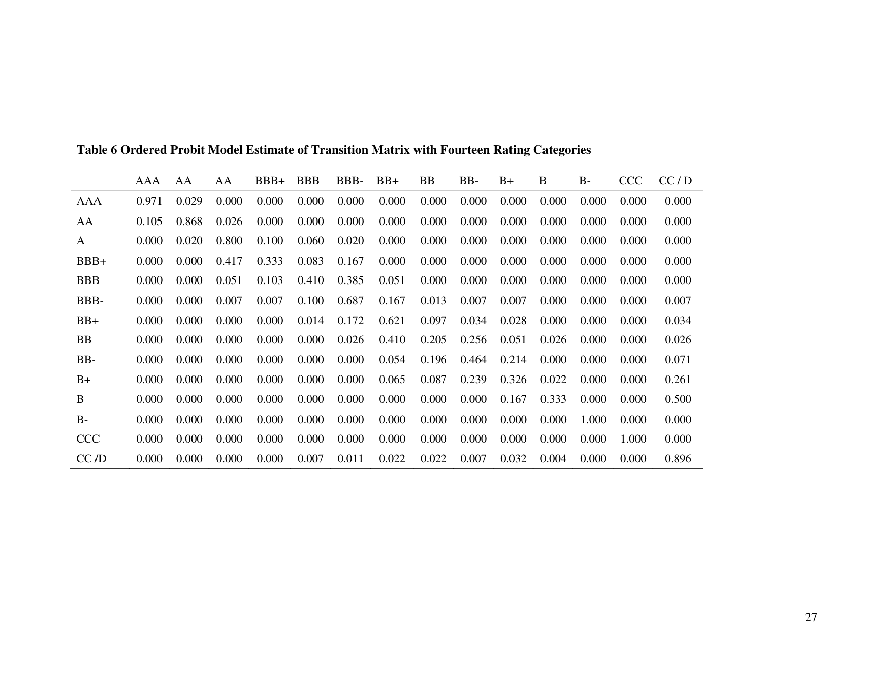
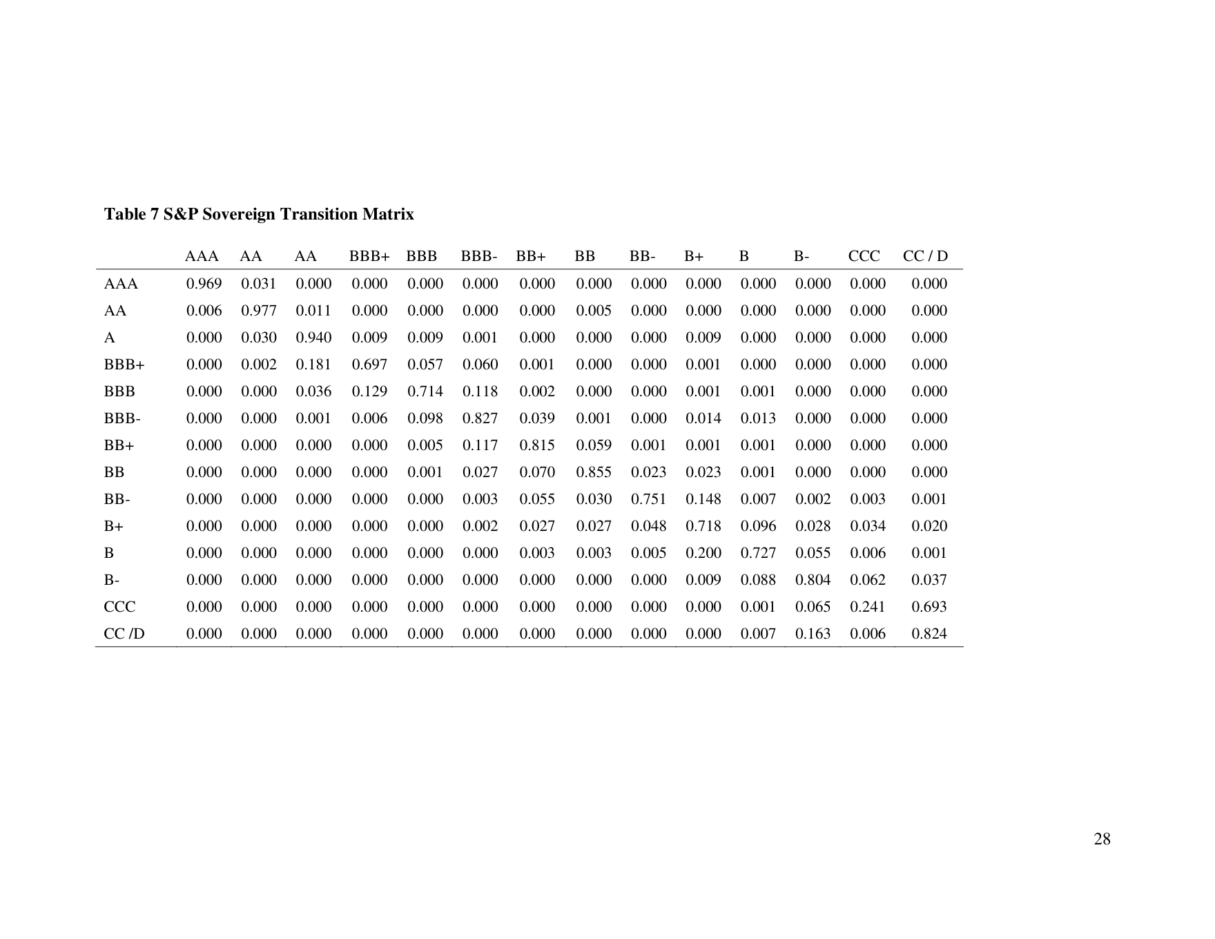
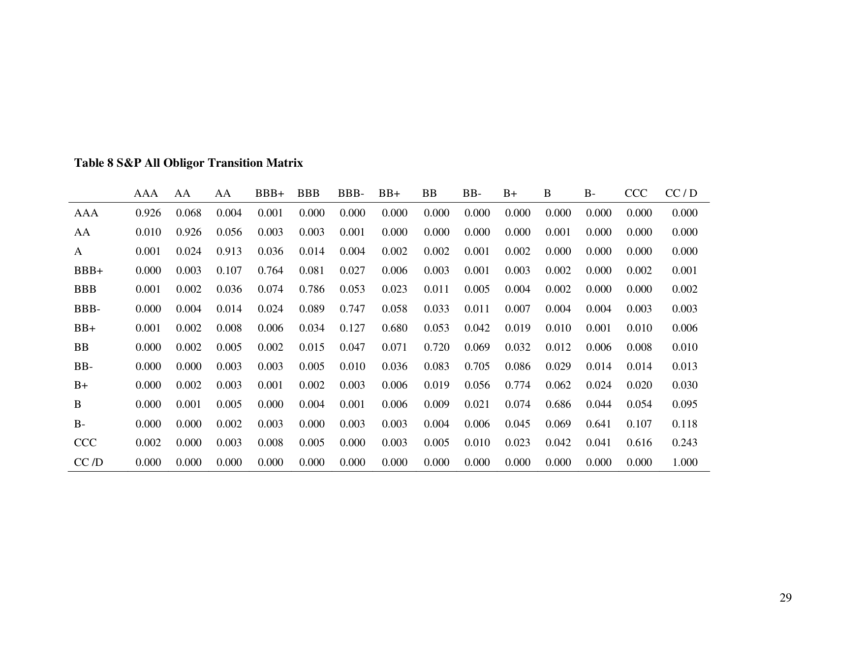
The results of these calculations for the coarse and the fine rating categories respectively are the matrices labelled “ordered probit estimates” in Table 3 and Table 6. In both of these tables, we also report simple, alternative estimates of the corresponding rating transition matrices, based solely on raw transition data (i) for sovereigns and (ii) for all obligors. Here, the all-obligor transition matrix is an estimate published by Standard and Poor’s that is calculated in the usual way by setting transition probabilities of moving from state i to state j equal to the relative frequencies of moving between these two states over a one year time period. In contrast, the sovereign matrix is calculated by (i) estimating the quarterly transition matrix (i.e., taking probabilities as equal to relative frequencies over quarterly periods) and then (ii) taking the fourth power of the resulting matrix to obtain an estimate of an annual transition matrix.[5]
In the case of the coarse ratings shown in Table 3, the probit-estimate matrix exhibits greater volatility of rating changes than the simple Standard and Poor’s transition matrix estimate in that diagonal elements of the probit-estimate matrix are generally smaller than those of the Standard and Poor’s matrix. This is particularly the case for the low rating categories such as B. Nevertheless, the estimated transition matrices are reasonably similar. The ordered probit estimates are more plausible in the AAA-A region. For example, the AA row of the matrix has entries grouped around the diagonal in the probit model estimates while the raw Standard and Poor’s estimates include offdiagonals entries only in positions far from the diagonal.
Note that in both the probit-model matrix and the Standard and Poor’s matrix, the CCC transition probabilities are shown as zeros except for the probability of no rating change. This reflects our convention that if there are no observations in a particular category, we place unity in the corresponding diagonal position in the matrix.
Tables 6, 7 and 8 show ordered probit and Standard and Poor’s transition matrices for sovereign obligors and all obligors based on the fine rating category data. Again, the ordered probit results are broadly similar to the raw Standard and Poor’s matrix for sovereigns although there is again somewhat more volatility (i.e., weight on offdiagonal entries). Again, there are problems with lowest non-default rating categories in that there were no observations of B- or CCC ratings.
6. A Bayesian Approach to the Estimation of Transition Matrices.
To combine information from the Standard and Poor’s estimate and the ordered probit estimate of transition matrices, we employ a Bayesian approach. The techniques we employ are related to Bayesian methods for estimating cell probabilities in contingency tables. As in our case, standard maximum likelihood estimators are unsatisfactory for estimating contingency tables since there are many cells and few observations per cell. Typically the empirical table seems too abrupt, and one may want to smooth the observed counts.
Such smoothing would allow the estimator to assign non-zero one-year transition probabilities even if there are no transitions observed within the sample. One could view the semi-parametric multiplicative hazard model used in the Lando and Skodeberg
(2001) article as a comparable methodology. While we smooth a transition matrix their baseline intensity is changed via a function of a covariate.
A widely used approach within the context of contingency table analysis is to employ a pseudo-Bayes technique, that is: (i) specify an appropriate prior and (ii) update it with a new estimator based on the observed data. Adapting this to the problem of estimating a
Markov chain transition matrix, one may write an estimator Pe based on a prior and an update as
= αQ + 1(−α) P . (4) Pe
Here, Q is the prior, in our case an empirical transition matrix estimated directly from Standard and Poor’s data and P is the estimator we obtain using the ordered probit method. Since the matrix Q is itself an estimator of the true transition matrix, up-dating this using other information actually corresponds to a pseudo (or empirical) Bayes approach.
The problem then reduces to one of selecting an appropriateα . In principle, there are three possibilities:
(i) A global approach based on a goodness of fitχ statistic.
(ii) A local approach looking at each row individually also based on goodness of fit statistics.
(iii) A cross-validation procedure in which α is chosen according to minimize some loss functional. The idea here is to drop one observed transition at a time, calculate the estimator based on all data without this observation, and then compare the prediction of the estimator with the true observation. All three procedures are well established and widely used. Procedure (i) is often called a “testimator” because it is based on a standard goodness of fit test (see Duffy and Santner (1989)). Procedure (ii) is described in Bishop, Fienberg, and Holland (1975), and compared with several other approaches. Procedure (iii) is a data-intensive procedure (see the discussion in Hall, Sheather, Jones and Marron, (1991)) and useful for larger datasets.
In general, Pseudo-Bayes estimators may be preferred to standard estimates because they have the same asymptotic performance but perform better in small samples (see Bishop, Fienberg, and Holland (1975)). Since the size of our data set is relatively small (in some cases the rating class considered has fewer than 30 observations), we prefer the goodness of fit procedures (i) and (ii) to the cross-validation approach, (iii), which tends to work better for larger data sets. Of the two goodness-of-fit procedures, (ii) seems preferable since it is more flexible, allowing for different weighting factors for each row of the transition matrix. (In the contingency table applications for which these methods were originally developed, the rows and columns collectively sum to unity and hence one may prefer to use a global approach yielding a single weighting factor for prior and update. In the transition matrix case, individual rows sum to unity and one may well wish to treat the rows of the matrix separately.)
To understand how the goodness of fit estimator (ii) works, let v(i) denote the number
of observations with initial rating i and let Yij denote the number of transitions from
rating i to rating j. The weighting factor, αi , for an individual row is then estimated by:
2 2 ˆ v ( i ) − Y ij K i ˆ ∑ j αi = where K i =[2] . (5) ˆ (Y − v ( i ) q ) v ( i ) + K i ∑ ij ij j Here qij is the ijth element of the matrix Q. Note the sense in which the weights are
chosen according to a modified goodness of fit procedure. If the prior fits the observations well, it will have a larger weight.
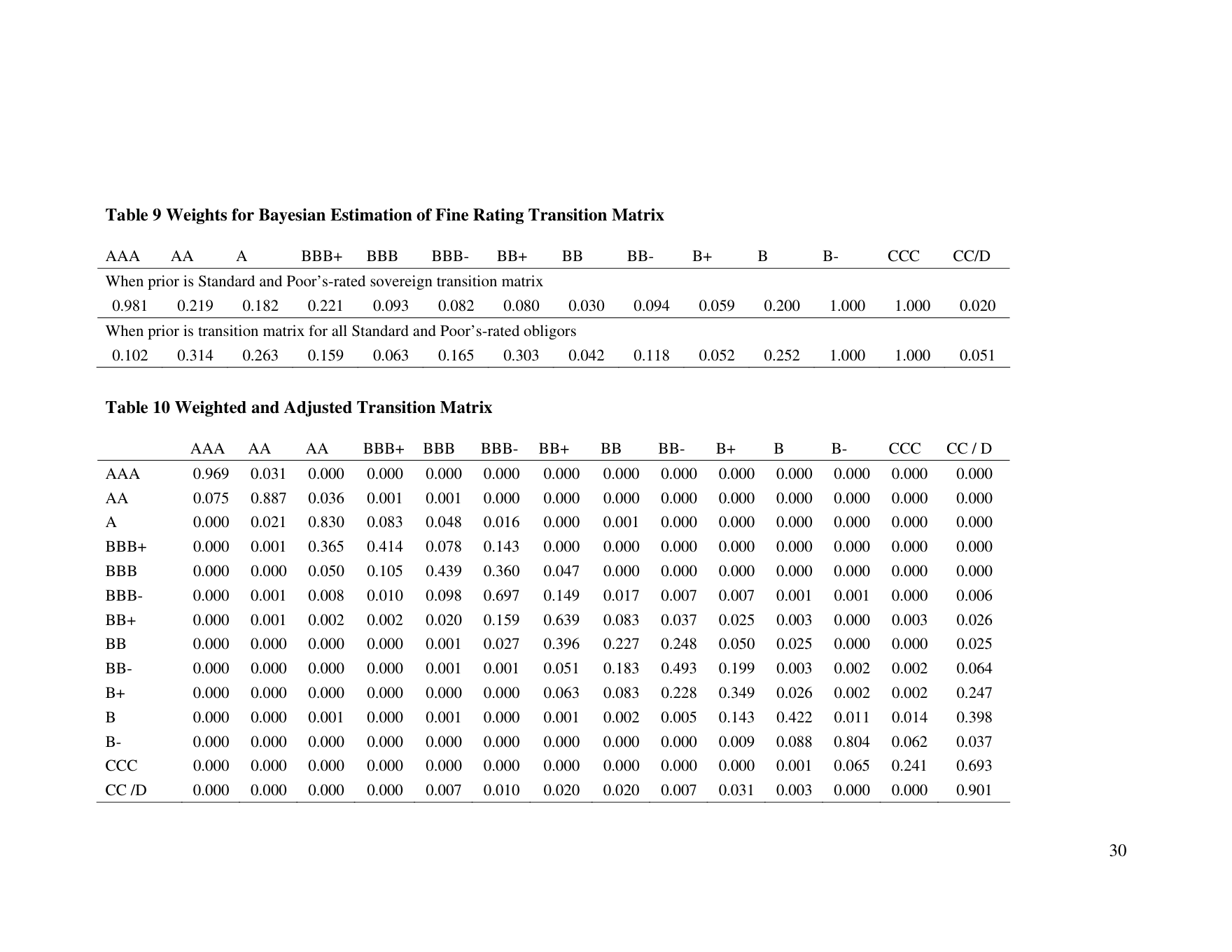
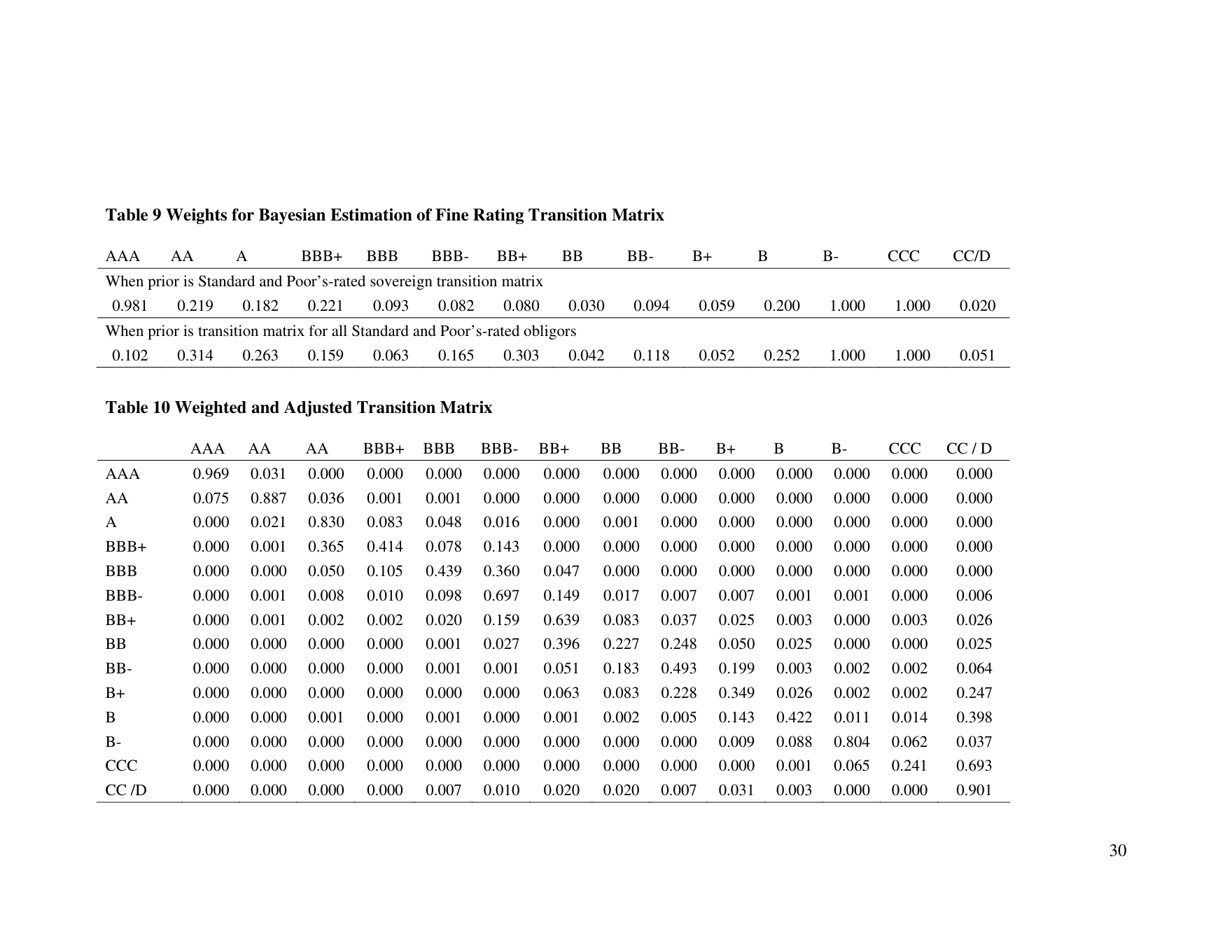
The weights obtained by the above method (ii) are shown in Table 5 for the coarse rating categories and 9 in the case of the fine ratings. In these tables, we show the weighting factors that the data suggests when we use either the Standard and Poor’s empirical transition matrix for sovereigns or the matrix for all Standard-and-Poor’srated obligors. The weights vary substantially across different rating categories, further justifying our choice of technique (ii) rather than (i). For some high rating categories, the prior fits the data so well that it receives a large weight. To construct a prior for a given row, we chose a row either of the sovereign or of the all-obligor matrix depending on which has the larger weighting factor, and then combine it with the probit model transition matrix using the weighted average formula given above.
Even after taking weighted averages, a problem remains with our Bayesian estimates of transition matrices in that the CCC rating category in the case of the coarse matrices, and both CCC and B- in the case of fine rating matrices are absorbing states. This reflects our convention that placing unity in the diagonal entry when no observations fall into that category. The most obvious way to remove this problem and generate a transition matrix which we can employ in practice in credit risk modelling is to suppose that the transition probabilities in the cases for which we do not observe transitions equal those of the naïve Standard and Poor’s sovereign transition matrix.
Table 4 and 10 show the Bayesian, weighted average transition matrices for coarse and fine rating categories, adjusted by replacing the CCC row with a row from the Standard and Poor’s naïve sovereign transition matrix in the coarse rating matrix and similarly replacing the CCC and B- rows in the fine rating matrix.
7. Evaluation of Model Performances
Table 11 shows the ratings of all the sovereigns in our estimating data set based on the probit model estimates and on Standard and Poor’s data where these are available. There is reasonably strong association between the ratings given by the model and the Standard and Poor’s ratings. If one converts the fine ratings to a numerical index, the correlation between the fitted ratings and the Standard and Poor’s ratings for all the years in our sample period is 82%. Nevertheless, there are significant differences for some countries.
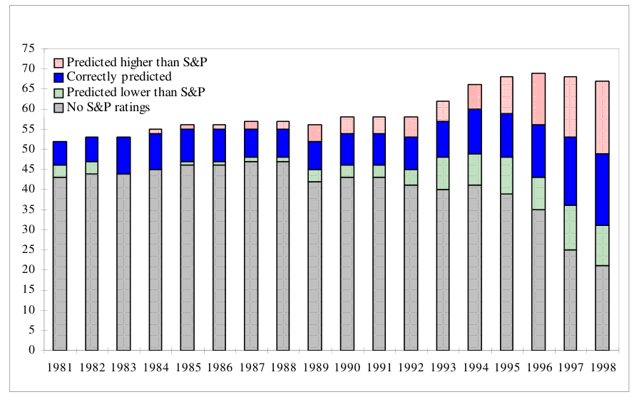
To examine how well the model fits the default and ratings data, we calculated (a) how many of the annual observations of sovereigns were correctly classified as defaults/nondefaults and (b) how many of the annual sovereign observations received the same rating from our procedure as they obtain from Standard and Poor’s. The results of these calculations broken down by year are shown in Figures 3 and 4.
Figure 3 indicates that our model fits the default data very well. The overwhelming fraction of annual sovereign observations are correctly classified between the default and non-default categories and this is true throughout the sample period. The only exception was in 1993 when the model somewhat under-predicted the number of sovereigns that emerged from default. Aggregating all the years, 95.04% of observations were correctly predicted, 2.43% of observations were predicted to be in default when they were not and 2.53% were predicted to be not in default when they were.
Figure 4 shows the number of sovereigns that are not rated by Standard and Poor’s and then breaks down the numbers that are rated into those which obtain the same rating from our procedure, and those which are rated higher and lower. The results suggest that our rating procedure is “unbiased” in the sense that roughly as many observations receive higher ratings from our procedure that from Standard and Poor’s as those that receive lower ratings. Again, aggregating years, 50.45% of observations were correctly rated, 22.85% had lower predicted ratings and 26.71% had higher predicted ratings than the actual Standard and Poor’s ratings.
Note that one should not evaluate our model by asking how well it fits the Standard and Poor’s ratings. Effectively, we estimate a model of actual default and then define rating categories broadly consistent with those employed by Standard and Poor’s. Given that we fit the default data rather well, the fact that there are a fairly large number of inconsistencies between our ratings and those of Standard and Poor’s suggests that our ratings may contain different but still highly relevant information about sovereign credit quality.
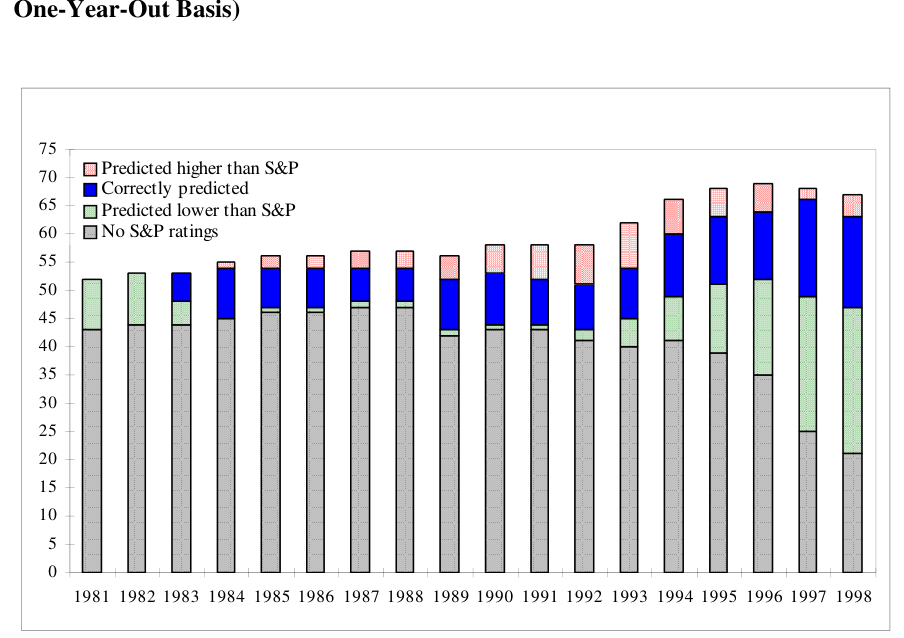
Figures 5 and 6 are the equivalent of Figures 3 and 4 except that the calculations are performed on a leave-one-year-out basis rather than a fully in-sample basis. By leaveone-year-out, we mean that to calculate the number of correctly classified observations in a particular year, we re-estimate the ordered probit model excluding data from that year and then use the resulting model to forecast what category the year-t observations should be in. This approach is in the spirit of the “leave-one-out method” discussed by Hand (1997).
Figure 5 shows that even on a leave-one-year-out basis, the model still fits the default data rather well and indeed there is very little difference between Figures 3 and 5. 94.86% of the default observations were correctly classified while 2.62% and 2.53% of observations were, respectively, predicted to be in default when they were not and predicted to be not in default when they were. Figure 6 on the other hand, does appear somewhat different from Figure 4 in that the ratings produced by the model are more conservative in the period up to and including 1998. In this case, 44.81% of observations were correctly rated, and 36.50% and 18.69% were respectively predicted lower or higher than the Standard and Poor’s ratings, respectively. While one might suggest that this represents a bias in the way in which the model is benchmarked against the Standard and Poor’s ratings, it is probably equally reasonable to argue that the model out-performed Standard and Poor’s in this period since it gave more conservative results just prior to the Asian and Russian crises.
8. Conclusion
This paper describes how one may improve upon raw estimates of rating transition matrices for Standard and Poor’s rated sovereigns by estimating a simultaneous ordered probit model of sovereign rating and default experience. Since data on sovereign defaults is available for a larger group of countries and over a considerably longer period than is sovereign rating data, this approach adds a significant amount of information about sovereign credit quality.
Given estimates of transition matrices based on our ordered probit model, we show how these may be combined with information in rating transition matrices calculated in a more conventional way from the wider population of Standard and Poor’s ratings histories. Formally, our approach of combining information represents an empirical or quasi-Bayesian procedure. We employ data-driven techniques for choosing appropriate weighting factors between our sovereign transition matrix estimate, one based on raw Standard and Poor’s transition data and one based on transition data for all Standard and Poor’s-rated obligors. We include a comparison of the ratings (and thus default probabilities) implied by our model with those attributed to different sovereigns by Standard and Poor’s.
Our analysis of the goodness of fit of our model to the default and ratings data suggests that it correctly classifies sovereigns as in default or not in default in an accurate fashion. The ratings produced by the model are benchmarked against the Standard and Poor’s ratings in an unbiased fashion except at the end of the sample period when the agency ratings were probably insufficiently conservative about sovereign risk in the run up to the Asian and Russian crises.
Bibliography
Bishop, Y. M. M., S. E. Fienberg, and P. W. Holland, (1975) Discrete Multivariate Analysis: Theory and Practice, MIT Press.
Burton, F.N. and H. Inoue, (1985) “The Influence of Country Factors on the interest differentials on International Lendings to Sovereign Borrowers,” Applied Economics, 17, 491-507.
Cantor, R. and F. Packer, (1996) “Determinants and Inputs of Sovereign Credit Ratings,” FRBNY Economic Policy Review, 2(2), 37-53.
Demirguc-Kunt, A. and E. Detragiache, (1998) “Determinants of Banking Crisis in Developing and Developed Countries.” IMF Staff Papers.
Duffy, D.E. and T. J. Santner, (1989) The Statistical Analysis of Discrete Data, Springer.
Edwards, S., (1986) “The Pricing of Bonds and Bank Loans in International Markets,” European Economic Review, 30, 565-89.
Edwards, S., (1984) “LDC Foreign Borrowing and Default Risk: An Empirical Default Risk, 1976-1980,” American Economic Review, 74, 726-34.
Eichengreen, B. and A. Mody, (1998) “What Explains Changing Spreads on Emerging Market Debt? Fundamentals or Market Sentiment?” NBER Working Paper, No.6408.
Feder, G., and R.E. Just, (1977) “A Study of Debt Serving Capacity Applying Logit Analysis,” Journal of Development Economics, 4, 25-38.
Greene, W. H., (1997) Econometric Analysis, Prentice Hall, 3rd edition.
Hall, P., S. J. Sheather, M. C. Jones and J. S. Marron, (1991) “On the optimal databased bandwidth selection in kernel density estimation.” Biometrika, 78, 262-69.
Hand, D.J., (1997) Construction and Assessment of Classification Rules, John Wiley & Sons, Chichester.
Haque, N.U., M. Kumar, N. Mark, and D. Mathieson, (1996) “The Economic Contents of Indicators of Developing Country Creditworthiness,” IMF Staff Papers, 43(4), 688- 724.
Jackson, P. and W. Perraudin, (2000) “Regulatory Implications of Credit Risk Modelling.” Journal of Banking and Finance, 24(1-2), 1-14.
Juttner, J.D. and J. McCarthy, (1998): “Modelling a Rating Crisis”, Macquarie University, Sydney, unpublished.
Kamin, S. and K. Kleist, (1999) “The Evolution and Determinants of Emerging Market Credit Spreads in the 1990s,” BIS Working Paper.
Lando, D. and T. Skodeberg, (2001) “Analyzing Ratings Transitions and Rating Drift with Continuous Observations,” forthcoming, Journal of Banking & Finance.
Min, H. (1998), “Determinants of emerging market bond spreads: Do economic fundamentals matter?” World Bank working paper.
Monfort, B. and C. Mulder, (2000) “Using Credit Ratings for Capital Requirement on Lending to Emerging Market Economies: Possible Impact of Basel Accord.”, IMF Working Paper, March.
Nickell, P., W. Perraudin and S. Varotto, (2000) “Stability of Rating Transitions” Journal of Banking and Finance, 24, 203-27.
Korea, Republic of 1998 BBB- BB+ BB+ to BBB- BBB+ to A A to AA Latvia, Republic of 1998 A BBB BBB+ BBB to BBB+ BBB Lesotho 1998 BB+ . . BBB- . Lithuania, Republic of 1998 A BBB- BBB to BBB+ BB to BB+ BBB- Malaysia 1998 BB+ A BBB BBB- to BBB A Maldives 1998 BBB- . . BB+ to BBB- . Mauritius 1998 BB+ . . BBB- to BBB . Mexico 1998 BB+ BB BB to BB+ B to B+ BB to BB+ Moldova, Republic of 1998 BB+ . . BB+ to BBB- . Mongolia 1998 BB . . B to B+ . Morocco 1998 BB+ BB BB to BB+ B- to B . New Zealand 1998 AAA AA AA to AAA AA to AAA AA Nigeria 1998 BB+ . . CC/SD to CCC . Norway 1998 AAA AAA AAA AAA AAA Pakistan 1998 BB B- B+ BB to BB+ B+ Panama 1998 BB BB+ BB to BB+ CC/D BB+ Papua New Guinea 1998 BB- . . BB- to BB . Paraguay 1998 BBB+ BB- BB+ to BBB- BBB- to BBB BB- Peru 1998 CC/D BB B CC/D . Philippines 1998 BB+ BB+ BB+ B to B+ BB- to BB Poland, Republic of 1998 BBB BBB- BBB- to BBB B- BB+ to BBB- Romania 1998 BB B+ BB- B+ to BB- BB- Seychelles 1998 BBB . . BBB to BBB+ . Slovak Republic 1998 BBB- BBB- BBB- BBB- to BBB BBB- South Africa 1998 BBB BB+ BBB- BBB+ to A BB to BB+ Spain 1998 AA AA AA AA to AAA AA Sri Lanka 1998 BBB- . . BB to BB+ . Thailand 1998 BB BBB- BB+ BB+ to BBB- A Trinidad and Tobago 1997 BBB- BB+ BB+ to BBB- B to B+ BB+ Tunisia 1998 BB+ BBB- BB+ to BBB- BB to BB+ BBB- Turkey 1998 B+ B B to B+ B to B+ BB- to BB United Kingdom 1998 AAA AAA AAA AAA AAA Uruguay 1998 BBB- BBB- BBB- B to B+ BB+ to BBB- Venezuela 1998 BB B+ BB- B- to B B+ to BB- Zambia 1998 CC/D . . CC/D . Zimbabwe 1998 B+ . . BB- to BB .
AAA AA A BBB+ BBB BBB- BB+ BB BB- B+ B B- CCC CC/D
Figure 2 The Number of Sovereigns in Default (based on ECGD Data)
70 Predicted default, actual non-default 65 Correctly predicted 60 Predictednon-default, actual default
1981 1982 1983 1984 1985 1986 1987 1988 1989 1990 1991 1992 1993 1994 1995 1996 1997 1998
Figure 4 Annual Sovereign Observations of Coarse Ratings
70 Predicted default, actual non-default 65 Correctly predicted 60 Predictednon-default, actual default
1981 1982 1983 1984 1985 1986 1987 1988 1989 1990 1991 1992 1993 1994 1995 1996 1997 1998
Figure 6 Annual Sovereign Observations of Coarse Ratings (Leave-One- Year-Out
| Parameters | Estimates | Std. Err. | Estimates | Std. Err. | |
|---|---|---|---|---|---|
| Constant | 1.054 | 0.129 | 1.034 | 0.127 | |
| Previous Year | Default Dummy | -2.751 | 0.271 | -2.668 | 0.260 |
| Debt to GNP | -2.451 | 0.374 | -2.388 | 0.362 | |
| Reserves to | Imports | 2.673 | 0.974 | 2.608 | 0.969 |
| Inflation | -1.925 | 0.587 | -1.833 | 0.570 | |
| Dummy for | Non-Industrial Countries | -2.244 | 0.260 | -2.277 | 0.259 |
| Lagged Debt | Service to Export | -2.503 | 0.666 | -2.317 | 0.646 |
| Lagged Inflation | -0.640 | 0.354 | -0.663 | 0.351 | |
| Cut-off point | 1 | 0.001 | 0.146 | 0.002 | 0.072 |
| Cut-off point | 2 | 0.683 | 0.075 | -0.001 | 0.125 |
| Cut-off point | 3 | 1.105 | 0.062 | 0.342 | 0.084 |
| Cut-off point | 4 | 0.893 | 0.063 | 0.603 | 0.076 |
| Cut-off point | 5 | 1.130 | 0.084 | 0.626 | 0.068 |
| Cut-off point | 6 | 1.174 | 0.066 | 0.504 | 0.065 |
| Cut-off point | 7 | 0.705 | 0.061 | ||
| Cut-off point | 8 | 0.708 | 0.063 | ||
| Cut-off point | 9 | 0.440 | 0.071 | ||
| Cut-off point | 10 | 0.308 | 0.076 | ||
| Cut-off point | 11 | 1.129 | 0.084 | ||
| Cut-off point | 12 | 1.172 | 0.066 | ||
| Average log | likelihood | -11.527 | -11.629 | ||
| Number of | cases | 1069 | 1069 |
| AAA | AA | A | BBB | BB | B | CCC | CC / D | |
|---|---|---|---|---|---|---|---|---|
| AAA | 0.978 | 0.022 | 0.000 | 0.000 | 0.000 | 0.000 | 0.000 | 0.000 |
| AA | 0.077 | 0.897 | 0.026 | 0.000 | 0.000 | 0.000 | 0.000 | 0.000 |
| A | 0.000 | 0.019 | 0.808 | 0.173 | 0.000 | 0.000 | 0.000 | 0.000 |
| BBB | 0.000 | 0.000 | 0.045 | 0.798 | 0.152 | 0.000 | 0.000 | 0.005 |
| BB | 0.000 | 0.000 | 0.000 | 0.106 | 0.776 | 0.078 | 0.000 | 0.041 |
| B | 0.000 | 0.000 | 0.000 | 0.000 | 0.327 | 0.367 | 0.000 | 0.306 |
| CCC | 0.000 | 0.000 | 0.000 | 0.000 | 0.000 | 0.000 | 1.000 | 0.000 |
| CC / D | 0.000 | 0.000 | 0.000 | 0.022 | 0.050 | 0.032 | 0.000 | 0.896 |
| S&P | Sovereign | Transition | Matrix | |||||
| AAA | AA | A | BBB | BB | B | CCC | CC / D | |
| AAA | 0.969 | 0.031 | 0.000 | 0.000 | 0.000 | 0.000 | 0.000 | 0.000 |
| AA | 0.006 | 0.977 | 0.011 | 0.000 | 0.006 | 0.000 | 0.000 | 0.000 |
| A | 0.000 | 0.030 | 0.939 | 0.020 | 0.001 | 0.010 | 0.000 | 0.000 |
| BBB | 0.000 | 0.000 | 0.033 | 0.926 | 0.024 | 0.017 | 0.000 | 0.000 |
| BB | 0.000 | 0.000 | 0.001 | 0.057 | 0.885 | 0.056 | 0.001 | 0.000 |
| B | 0.000 | 0.000 | 0.000 | 0.002 | 0.063 | 0.886 | 0.031 | 0.018 |
| CCC | 0.000 | 0.000 | 0.000 | 0.000 | 0.001 | 0.066 | 0.241 | 0.693 |
| CC / D | 0.000 | 0.000 | 0.000 | 0.000 | 0.005 | 0.169 | 0.003 | 0.823 |
| S&P | Transition Matrix | for All | Rated | Obligors | ||||
| AAA | AA | A | BBB | BB | B | CCC | CC / D | |
| AAA | 0.926 | 0.068 | 0.004 | 0.001 | 0.000 | 0.000 | 0.000 | 0.000 |
| AA | 0.006 | 0.918 | 0.068 | 0.006 | 0.001 | 0.001 | 0.000 | 0.000 |
| A | 0.001 | 0.024 | 0.918 | 0.050 | 0.005 | 0.002 | 0.000 | 0.000 |
| BBB | 0.000 | 0.003 | 0.054 | 0.885 | 0.046 | 0.009 | 0.001 | 0.002 |
| BB | 0.000 | 0.001 | 0.005 | 0.071 | 0.823 | 0.079 | 0.011 | 0.010 |
| B | 0.000 | 0.001 | 0.003 | 0.005 | 0.060 | 0.832 | 0.039 | 0.058 |
| CCC | 0.002 | 0.000 | 0.003 | 0.013 | 0.018 | 0.106 | 0.616 | 0.243 |
| CC / D | 0.000 | 0.000 | 0.000 | 0.000 | 0.000 | 0.000 | 0.000 | 1.000 |
| AAA | AA | A | BBB | BB | B | CCC | CC / D | |
|---|---|---|---|---|---|---|---|---|
| AAA | 0.972 | 0.028 | 0.000 | 0.000 | 0.000 | 0.000 | 0.000 | 0.000 |
| AA | 0.049 | 0.906 | 0.042 | 0.003 | 0.000 | 0.000 | 0.000 | 0.000 |
| A | 0.000 | 0.020 | 0.828 | 0.151 | 0.001 | 0.000 | 0.000 | 0.000 |
| BBB | 0.000 | 0.000 | 0.046 | 0.805 | 0.143 | 0.001 | 0.000 | 0.005 |
| BB | 0.000 | 0.000 | 0.001 | 0.097 | 0.788 | 0.078 | 0.003 | 0.033 |
| B | 0.000 | 0.000 | 0.000 | 0.000 | 0.317 | 0.385 | 0.001 | 0.297 |
| CCC | 0.000 | 0.000 | 0.000 | 0.000 | 0.001 | 0.066 | 0.241 | 0.693 |
| CC / D | 0.000 | 0.000 | 0.000 | 0.021 | 0.048 | 0.031 | 0.000 | 0.900 |
| AAA | AA | A | BBB | BB B | CCC |
|---|---|---|---|---|---|
| is Standard | and | Poor’s-rated | sovereign | transition matrix | |
| 0.656 | 0.293 | 0.129 | 0.049 | 0.085 0.031 | 1.000 |
| is the | transition matrix | for all | Standard and | Poor’s-rated obligors | |
| 0.060 | 0.399 | 0.181 | 0.083 | 0.251 0.037 | 1.000 |
| Country | Names | End | of Sample | Period | Ratings | Average | Ratings in | the | |
|---|---|---|---|---|---|---|---|---|---|
| Year Our | Model | S&P | Average | Our Model | S&P | ||||
| Algeria | 1998 | BB | . | . | CCC to | B- | . | ||
| Argentina | 1998 | BB | BB | BB | B to B+ | BB- | to | ||
| Australia | 1998 | AAA | AA | AA to | AAA | AAA | AA | ||
| Austria | 1998 | AAA | AAA | AAA | AAA | AAA | |||
| Bangladesh | 1998 | BBB- | . | . | BBB- | . | |||
| Barbados | 1998 | BBB+ | . | . | BBB- to | BBB | . | ||
| Belize | 1998 | BBB- | . | . | BBB- to | BBB | . | ||
| Bolivia | 1998 | CC/D | . | . | CC/D | . | |||
| Botswana | 1998 | A | . | . | A | . | |||
| Brazil | 1998 | BB | BB- | BB- to | BB | CCC to | B- | B+ | |
| Bulgaria | 1998 | CC/D | . | . | CC/D | . | |||
| Cameroon | 1997 | CC/D | . | . | CC/D | . | |||
| Chile | 1998 | BBB- | A | BBB to | BBB+ | BB to | BB+ | BBB+ to | |
| Colombia | 1998 | BB+ | BBB- | BB+ to | BBB- | BB to | BB+ | BBB- | |
| Costa Rica | 1998 | BBB- | BB | BB+ | B- to | B | . | ||
| Croatia, | Republic of | 1998 | BBB- | BBB- | BBB- | B to B+ | BBB- | ||
| Czech Republic | 1998 | BBB- | A | BBB to | BBB+ | BBB- to | BBB | BBB+ to | |
| Denmark | 1998 | AAA | AA | AA to | AAA | AAA | AA | ||
| Dominican | Republic | 1998 | BBB | B+ | BB to | BB+ | B- to | B | B+ |
| Ecuador | 1998 | CC/D | . | . | CCC to | B- | . | ||
| Egypt, Arab | Republic of | 1998 | BBB | BBB- | BBB- to | BBB | B+ to | BB- | BBB- |
| El Salvador | 1998 | A | BB | BBB- to | BBB | BB to | BB+ | BB | |
| Estonia, | Republic of | 1998 | A | BBB+ | BBB+ | to A | BBB to | BBB+ | . |
| Finland | 1998 | AA | AA | AA | AA to | AAA AA | to AAA | ||
| Germany | 1998 | AAA | AAA | AAA | AAA | AAA | |||
| Ghana | 1998 | CC/D | . | . | CCC to | B- | . | ||
| Hungary | 1998 | BB- | BBB- | BB to | BB+ | B to B+ | BB+ | to | |
| Iceland | 1998 | AA | A | A to | AA | AA | A | ||
| India | 1998 | BBB- | BB+ | BB+ to | BBB- | BBB- | BB+ | ||
| Indonesia | 1998 | CC/D | CCC | CC/SD | to CCC | BB- to | BB BBB- | to | |
| Iran, Islamic | Republic of | 1982 | A | . | . | . | . | ||
| Jamaica | 1998 | BB+ | . | . | B+ to | BB- | . | ||
| Japan | 1990 | AAA | AAA | AAA | AAA | AAA | |||
| Jordan | 1998 | B+ | BB- | B+ to | BB- | CC/SD to | CCC B+ | to BB- | |
| Kazakhstan, | Republic of | 1998 | BBB | BB- | BB+ | B+ | BB- |
Notes
[1] By “the number of annual observations” we mean the total, summed over the different years in the sample, of sovereigns rated on 5th July.
[2] Our approach requires that we have no missing variables among a set of macroeconomic and financial regressors that we use to model credit quality. Of the1069 valid observations with no missing data, there are 337 annual observations of Standard and Poor’s sovereign ratings of which only 131 were sub single A rated. The number of annual rating change observations was 21 or 11 excluding those for which the initial rating was less than single A.
[3] An alternative would have been to use the logit model employed by, for example, Demirguc and Kunt (1998) and Feder and Just (1977) to estimate default probabilities.
[4] To be precise, our dependent variables are based on (i) ratings observed on July 5th of a year with date t, (ii) a default dummy which is unity if there was a default at any point in the year with date t, and (iii) explanatory variables for the year t. Explanatory variables which are stocks like debt levels are measured on 1st January of any given year since this is the convention followed by the provider of these data, the World Bank, while rates of change on flow variables such as GDP growth are rates of change from t-1 to t of the year average levels.
[5] This simple trick of calculating a higher frequency transition matrix and then taking powers to obtain an annual matrix is very close in spirit to the continuous time approach advocated by Lando and Skodeberg (2001).