

A significant obstacle to the revival of the European securitisation market is the high level of capital that insurers are required to hold against securitisation positions under Solvency II rules. This paper presents evidence on how securitisation capital for insurers should be calibrated. We analyse a large dataset of price data on individual tranches, construct return indices and measure the Value at Risk of different securitisation portfolios. We also analyse capital from a bottom up perspective, allocating Solvency II capital for asset pools to securitisation tranches using the Simplified Supervisory Formula Approach (SSFA) employed in the Basel III rules. We conclude that Solvency II capital charges for AAA-rated Type 1 tranches are double what the evidence suggests is appropriate. Charges for Type 2 tranches are also much higher than is justified by the data.
1. Introduction
In designing the Solvency II rules, the European authorities have sought to align regulatory capital with the contribution that different exposures make to total balance sheet risk. Achieving this requires careful supervision of the internal models employed by advanced insurance firms but, also, appropriate calibration of the Standard Formula rules applied by other insurers.
A difficult area for calibration has proved to be capital for securitisations. The challenge of achieving satisfactory rules in this area is underlined by the fact that the European authorities have proposed three very different calibrations since 2010 and may be contemplating further changes in the securitisation capital rules that came into force, along with the rest of Solvency II, in January 2016.
The difficulty in calibrating rules for securitisations stems from the fact that misuse of securitisation in the US subprime market contributed significantly to the recent crisis. On the other hand, the European securitisation market proved relatively robust in the crisis, in that, despite substantial macroeconomic shocks, highly rated tranches in the main asset classes exhibited negligible defaults.[2]
Keen to bolster growth in Europe, policymakers have examined the contribution that a restored securitisation market might make in freeing up bank balance sheets and thereby creating room for lending. In April and May 2014, the Bank of England and the European Central Bank published two papers commenting on the possible benefits of reviving securitisations in Europe.[3] An obstacle to such a revival, identified by the central banks, is the conservative post-crisis capital rules for banks and insurers that hold securitisations.
Solvency II securitisation capital rules should ideally be calibrated using data relevant to their likely future performance. Such data are hard to come by, in that only relatively short runs of historical data are available. Furthermore, one might argue that post crisis reforms including skin-in-the-game and transparency requirements on issuers and regulation of ratings agencies have changed the market so that past and future data may not be fully comparable.
In this paper, we revisit past attempts by regulators to relate Solvency II capital charges to historical data on changes in securitisation values. To achieve this, we create a substantial dataset comprising all the securitisation positions listed on Bloomberg (including matured bonds), construct return indices for subsets of the securitisations based on ratings and proxy indicators for the Type 1 and Type 2 categories employed by Solvency II rules,[4] and then estimate capital using a Value at Risk (VaR) criterion.
Applying this relatively simple and transparent method, we show that, for AAArated Type 1 tranches and for Type 2 tranches more generally, capital charges should be much lower than those currently prescribed in Solvency II.
We also implement a look through approach to securitisation capital. In this case, we calculate Solvency II capital for pool assets and then split it between different tranches using the Simplified Supervisory Formula Approach (SSFA), the function employed for the same purpose by the Basel III framework. The version of the SSFA we employ implies a significant capital premium in the sense that the capital an insurer would have to hold if it owned all the tranches would be double the capital required if it held the pool assets.[5] The implied capital is, nevertheless, considerably lower than that implied by the current Solvency II capital rules.
The paper is organised as follows. Section 2 describes the sequence of securitisation capital calibrations that the European authorities have so far published. These include a quasi-look-through approach to calibration (based on Standard & Poor’s (S&P) rating methodologies) implemented in 2010, a market return-based calibration using historical data on Markit and Merrill Lynch securitisation indices completed in 2013 and a subsequent adjustment to the 2013 calibration adopted by the European Commission in 2015.
Section 3 describes our market price based calibration employing a large dataset of time series information on individual European securitisation tranches. This involves creating a set of return indices, random sampling with replacement of weekly returns in order to create a dataset of annual returns, and VaR calculations which yield per-year-of duration capital charges for securitisations by rating and distinguishing between Type 1 and Type 2 securitisation tranches.
Section 4 derives Solvency II capital charges (based on the calibration results implied by the previous section) inclusive of diversification adjustments. In the Solvency II Standard Formula, capital charges are specified for undiversified positions in individual exposure classes and, then, combined to obtain a charge for the balance sheet as a whole, using a correlation matrix for the different risks involved.
The implied capital charges depend on the assets held by the insurer in question. To estimate the all-in capital effects of different calibrations, we therefore formulate the stylised balance sheet of a representative European life insurer, and calculate the capital charges for different securitisations, both exclusive and inclusive of diversification adjustments.
This paper contributes to a growing series of research studies aimed at analysing the basis of capital regulation for insurers and banks. Several papers have looked at Solvency II calibration. Thibeault and Wambeke (2014) calculate and compare capital charges for different asset classes including securitisations using Basel and
Solvency II Formula approaches. Their paper, like ours, demonstrates that securitisation capital rules for European insurers are excessively conservative. Floreani (2012) criticises the treatment of diversification under Solvency rules, suggesting that it inadequately distinguishes between systemic and non-systemic risk and encourages insurers to diversify in ways that will boost the destabilising effects of systemic shocks.
Höring (2012) compares, for a stylised but representative European life insurer, the capital requirements implied by Solvency II rules with those employed in S&P rating criteria for insurers. He argues that the S&P criteria are the binding constraint and, therefore, Solvency II will not affect the portfolio choices of insurers. Arias, Arouri, Foulquier and Gregoir (2010) examine the appropriateness of the Solvency II calibration for private equity.
Pfeifer and Strassburger (2008) comment critically on the diversification adjustments employed within Solvency II rules. They argue that for a set of distributions for individual risk class returns, the Solvency II approach to diversification adjustment produces incorrect or unstable results. Mittnik (2011) is highly critical of the statistical techniques used in calibrating the equity exposure module of Solvency II, arguing that the overlapping observation methods applied lead to spurious results.
Also highly relevant for our study are a series of papers on the appropriateness of the Basel III securitisation capital regulations. The Basel proposals for securitisation capital rules evolved over the period 2013 to 2015. This evolution may be understood if one reads the sequence of Basel Committee publications BCBS 236, 269 and 303. In parallel, alternative approaches to designing capital charges and performing calibrations were advanced by Duponcheele, Perraudin and Totouom-Tangho (2013a) (2013b) (2014a) and (2014b), Duponcheele, Linden, Perraudin and Totouom-Tangho (2014), Duponcheele, Linden and Perraudin (2014) and (2015).
The European authorities are considering introducing a distinction, for the purpose of calculating bank capital, between high quality securitisations (denoted Simple, Transparent and Standardised (STS)) and others. See EBA (2015) and European Commission (2015). The distinction is along the lines of the Solvency II distinction between Type 1 and 2 securitisations, being based on a complex set of largely qualitative criteria.
2. Solvency II calibration
2.1. Introduction to calibration
In this section, we describe the approach the authorities have taken in calibrating Solvency II for securitisation exposures. We begin by explaining the design of the Standard Formula (SF) detailed in Directive 2009/138/EC and what this design implies about calibration. We then describe the successive attempts that the authorities have made to calibrating securitisation capital.
To understand how Solvency II SF charges for securitisations should be calibrated, one must grasp how this approach is designed. Key features of the SF include the following.
1. Capital charges for a portfolio consisting of exposures within a given risk class equal a weighted sum of the individual exposure values with the weights being invariant to the composition of the portfolio.
2. Capital charges for a portfolio comprising exposures to multiple risk classes are calculated (inclusive of an adjustment for diversification) as equalling the volatility of a set of risk-class-specific holdings.[6]
This approach is consistent with theory under the following assumptions. First, as is well-known (see Gordy (2003)), the Value-at-Risk of a portfolio equals a weighted sum of exposure amounts (with the weights being independent of the portfolio composition) only if the portfolio is perfectly granular and driven by a single common factor (all other idiosyncratic risk having been eliminated by diversification).
Second, given a portfolio of exposures to a set of asset returns, if the returns are jointly elliptically distributed, quantiles of the distribution of portfolio losses are proportional to the standard deviation of the portfolio value.
Hence, the Solvency II approach may be justified on the basis that (i) the insurer in question has a set of diversified exposures within each asset class, (ii) the returns for each asset class have a single common factor and (iii) that the joint distribution of the common factors is elliptical.
To calibrate this approach, one may then, first, base the capital weights for each risk class on the VaR of a diversified portfolio of exposures within that risk class and, second, use a correlation matrix to calculate total, enterprise capital (adjusted for diversification) using the portfolio volatility formula referred to above.[7]
In this paper, our concern will be with the first of these two calibration issues. We shall leave aside the issue of whether the correlation matrix employed by the authorities is appropriate. Hence, we focus on the issue: how may one estimate the VaR of a diversified portfolio of securitisation exposures assuming (consistent with the Solvency II approach) that the confidence level of the VaR is 99.5% and the holding period is 1 year?
2.2. The CEIOPS (2010) Calibration
In this and in the following two subsections, we explain the calibrations that have previously been proposed by the European authorities. An early calibration of the Solvency II capital charges for securitisations was provided by the Committee of
European Insurance and Occupational Pensions Supervisors (CEIOPS) in 2010.[8] This 2010 calibration may be found in CEIOPS-DOC-66/10.
Rather than using market data to calibrate capital for securitisation portfolios, CEIOPS derived capital by applying stress factors to underlying assets. This approach closely resembles that used by the ratings agency S&P. The calibration makes use of ‘AAA’ scenario default rates considered as a function of rating and tenure ranges. The function may be denoted G(Tenure, Rating). The values the function takes for different ratings and tenure ranges are shown in Table 1. A similar function for recovery rates, denoted R(Rating), may be defined based on the values shown in Table 2.
Under the CEIOPS (2010) approach, to calculate the risk factor for a particular securitisation position, one must, first, calculate the loss rate for the underlying assets using the formula:
∑G(Tenurei i,Ratingi)∙(1−R(Ratingi))∙MVi Lossrate= (1) MV
Here, Tenurei , Ratingi and MVi are the tenure, rating and market value respectively of underlying loan i, and MV is the total market value of the pool of underlying loans.
struct for the securitisation position is given by the The capital charge Mktsp expression:
Lossrate−Attacℎmentpoint struct = (2) Mktsp Detacℎmentpoint−Attacℎmentpoint struct. Finally, a floor of 10% and ceiling of 100% are applied to Mktsp
| Asset rating | |||||||||||
|---|---|---|---|---|---|---|---|---|---|---|---|
| Asset tenure | |||||||||||
| AAA | AA | A | BBB | BB | B | <B | Unrated | ||||
| (years) | |||||||||||
| 0 | ≤ | Tenure < | 2 | 0.8 | 1.6 | 4.7 | 8.1 | 20.9 | 41.5 | 65.9 | 9.7 |
| 2 | ≤ | Tenure < | 4 | 1.6 | 3.1 | 8.1 | 14.7 | 34.1 | 59.7 | 83.3 | 17.6 |
| 4 | ≤ | Tenure < | 6 | 2.3 | 5.0 | 10.9 | 20.2 | 43.0 | 68.2 | 88.4 | 24.2 |
| 6 | ≤ | Tenure < | 8 | 3.5 | 7.4 | 14.0 | 25.2 | 50.4 | 73.3 | 90.7 | 30.2 |
| 8 | ≤ | Tenure < | 10 | 4.7 | 9.7 | 17.1 | 30.2 | 56.2 | 77.1 | 91.9 | 36.2 |
Note: The ‘AAA’ scenario default rate is equal to the fraction of portfolio defaults that an AAA rated CDO tranche should be able to withstand, where the underlying assets are of a uniform credit quality and tenure. The calibration of these values is detailed in Standard and Poor’s (2009). The scenario default rates for unrated securitisations are based on the scenario default rates for BBB rated securitisations. Rates are given in percent.

Note: These values are provided in CEIOPS-DOC-66/10. Rates are given in percent.
2.3. The EIOPA (2013b) Calibration
The Solvency II capital charges for securitisation positions were completely recalibrated in 2013. The recalibration and the approach on which it is based are described in EIOPA (2013b).[9]
First, securitisation positions are divided into two categories: ‘Type A’ and ‘Type B’. Re-securitisations are treated separately. ‘Type A’ securitisation positions are those that meet a set of qualitative and quantitative requirements described in EIOPA (2013b). These requirements are summarised in Table 3.
In order to calibrate the capital charges for securitisation positions, components of the following indices obtained from Markit and Bank of America Merrill Lynch were used:
Floating rate Markit iBoxx European ABS indices:
• Markit iBoxx Prime RMBS Index (excluding Granite)
• Markit iBoxx Europe (excluding UK) RMBS Index
• Markit iBoxx Eurozone RMBS
• Markit iBoxx UK Non-Conforming RMBS Index
• Markit iBoxx UK Credit Card Index
• Markit iBoxx SME CLO Index
• Markit iBoxx CMBS Index
• Markit iBoxx Auto Loan Index
• Markit iBoxx Auto Lease Index
US fixed and floating rate and UK fixed rate ABS indices from BAML Global Index System:
• US ABS Master Fixed R0A0
• US ABS Master Floating R0F0
• US CMBS – CB10, CB20, CB30, CB40
• Fixed Rate Sterling Non-Gilt Securitized USEA
The above indices were mapped to either Type A or Type B, with those indices containing securitisations historically displaying lower spread risk being assigned to Type A.
First, aggregated spreads were calculated for each combination of rating[10] and type. Each aggregate spread was calculated by considering those indices assigned to the specified type, and taking the sum of the spreads of the component securitisations of the specified rating, weighted by market value. This was done separately for the Markit and BAML indices, with daily spread data being used for the Markit indices and monthly spread data being used for the BAML indices.
Next the annual change in each of the aggregated spreads was calculated each day for the Markit indices and each month for the BAML indices. The result is a set of overlapping observations of one-year changes in spread. For each rating/type pair the 99.5% VaR is then calculated using this data.
The last step was to combine the VaRs based on the Markit and BAML indices. For each rating/type pair the VaR was calculated as the weighted average of the VaRs calculated based on the Markit indices and the BAML indices, with a 95% weighting given to the Markit indices. This weighting was designed to match the ratio of European to US securitisation positions held in the portfolio of an average European insurer.
Let the one-year, spread based VaR for securitisation position i be denoted bi, and the modified duration[11] of the securitisation position equal duri . The capital charge is then set equal to the risk factor stress of the securitisation position, denoted stressi and equal to:
(3) stressi = bi ∙duri.
The risk factor stress, stressi, is capped at 100%. The value of bi for BBB rated Type A securitisations was set judgmentally for lack of available data. Table 4 gives the values of bi assigned to Type A and B securitisations.
| Seniority | (c) |
|---|---|
| Legal true sale | (d) |
| No severe clawback provisions | (e) |
| Servicing continuity | (f), |
| Eligible underlying assets | (h) |
| Homogeneous cash flows | (h) |
| Type of underlying asset | (i), |
| Rating requirements | (a) |
| No credit impairing | (k) |
| No non-performing loans | (l) |
| At least one payment | (p) |
| Listing requirement | (b) |
| Transparency, reporting and disclosure requirements | (t) |
| No self-certification | (q) |
| Process for assessing creditworthiness | (r), |
Note: The Type A securitisation requirements are shown in the first column of Table 3. The second column gives the corresponding paragraph of Delegated Regulation (EU) 2015/35, Article 177 (2).
| AAA | AA | A | BBB | BB | B | <B |
|---|---|---|---|---|---|---|
| 4.3 | 8.45 | 14.8 | 17-20 | - | - | - |
| 12.5 | 13.4 | 16.6 | 19.7 | 82 | 100 | 100 |
Note: These values are provided in Technical Report EIOPA/13/513. The capital charges shown are per year of duration and are given in percent.
2.4. Subsequent changes
Delegated Regulation (EU) 2015/35 sets out the current framework and calibration of capital for securitisations positions. The framework is now in force, following the implementation of Solvency II in January 2016.
Delegated Regulation (EU) 2015/35 refers to Type A and B securitisations by the revised labels Type 1 and 2. The requirements that securitisation exposures must meet to be Type 1 according to Delegated Regulation (EU) 2015/35 are broadly the same as the requirements for Type A securitisation positions given in Technical Report EIOPA/13/513 (see Table 3).
The most substantial changes relate to the definition of eligible underlying assets. Delegated Regulation (EU) 2015/35, Article 177 (2h) lays out explicit criteria that a securitisation backed by residential mortgages must meet in order for a tranche in that securitisation to qualify as Type 1.
In the technical specifications produced for the Solvency II preparatory phase (EIOPA-14/209), the risk factors for Type A securitisations (derived in Technical Report EIOPA/13/513) were halved. In the final implementation (Delegated Regulation (EU) 2015/35) a ceiling of 3% is applied to the value of bi for Type A securitisations. This is in line with the capital charges for unrated bonds (although it is still higher than for secured loans such as mortgages).
Table 5 gives the final values of bi (from Delegated Regulation (EU) 2015/35). The values of bi for Type 2 securitisation exposures in the final implementation are unchanged from those given in Table 4 for Type B securitisation exposures.
The pre-diversification capital charges set out in Table 5 appear highly questionable. Going from Type 1 to Type 2 often involves minor changes in qualitative features of deals. To raise the capital by a factor of four appears completely incommensurate with such differences between individual bonds.
The flat charge schedule for Type 1 tranches rated below AAA also appears unscientific. It is scarcely conceivable that credit quality declines from AA to BBB are not associated with higher risk and, therefore, meriting of higher capital. The objective of this study is to generate analysis which leads to a capital charge calibration that is more reasonable and prudent.
| AAA | AA | A | BBB | BB | B | <B |
|---|---|---|---|---|---|---|
| 2.1 | 3 | 3 | 3 | - | - | - |
| 12.5 | 13.4 | 16.6 | 19.7 | 82 | 100 | 100 |
Note: These values are provided in Delegated Regulation (EU) 2015/35. The capital charges shown are per year of duration and are given in percent.
3. Index analysis
3.1. Summary of VaR analysis
In this section, we describe our empirical analysis of securitisation risk. The analysis is based on an extensive dataset of information on European securitisation exposures collected primarily from Bloomberg.
Our objective is to generate a calibration consistent with the current Solvency II framework. Three aspects of the Solvency II approach are important in this:
1. The approach distinguishes between Type 1 and Type 2 securitisation exposures.
2. It differentiates between different rating categories.
3. Prior to diversification adjustment, the capital charge for a given position equals its value multiplied by the product of a fixed weight and its modified duration.
Aspect 3 has important implications for how one performs the calibration. First, the fact that, for given modified duration, capital consists of a set of fixed weights times the values of the positions, is consistent with a one-factor model of risk. Second, the assumptions that capital is homogeneous in modified duration is consistent with a model in which the portfolio comprises fixed income exposures for which spreads shift up or down in a parallel fashion over time. In calibrating the model, we make use of these assumptions.
In brief, our approach to Solvency II calibration consists of the following seven steps:
1. We calculate weekly log returns on individual securitisation positions.
2. We then divide the return by the modified duration of each position in order to obtain the 1-year-modified-duration-equivalent return (under the Solvency II homogeneity assumption).
3. For each period, we calculate the unweighted average of the 1-yearmodified-duration-equivalent returns for different categories of securitisation positions, thereby constructing time series of weekly portfolio returns.
4. Since our objective is to study risk over 1-year horizons, we randomly draw (with replacement) 52 weekly time periods. Summing these weekly returns generates a time series of annual returns.
5. Repeating Step 4 many times yields a dataset of annual returns from which one may calculate Value at Risk (VaR) for the portfolio in question.
6. The calculations are based on 1-year-modified-duration-equivalent returns and so the resulting VaR number is the capital charge for a securitisation position (i) with the same characteristics as the portfolio that has been analysed and (ii) with a 1 year modified duration.
7. To obtain the capital charge for a position with a modified duration of n years, we multiply the 1-year capital charge by n.
The time series we obtain though Step 3 may be regarded as a return index for the portfolio in question. Because we have constructed return indices ourselves, the exact nature of their constituents is transparent to us (which would not be true if we used published indices). As we shall see below, in securities markets of varying liquidity like the securitisation market, there may be shifts in the composition of the data available. This can influence calculations of risk statistics and requires careful treatment which is only possible if one is in a position to calculate the index from its security level constituents.
3.2. Data description
Our bond list contains all the European securitisation positions that appear in the Bloomberg database in the period up to September 30th 2013.[12] To define the nature of each position, we retrieve bond characteristics information of underlying asset class, tranche seniority and collateral country from Bloomberg. After eliminating bonds without valid characteristics information, our bond list contains a total of 8,322 eligible bonds.
Our bond positions fall into 6 categories according to their underlying asset types. The categorisation is described in Table 6. RMBS is the biggest category in our sample in terms of number of bonds, which account for 42% of our sample. Relatively risky securitisation positions, such as CMBS, leveraged CLOs and other CDOs, are also included in our sample.
Our portfolio comprises of positions both from countries that are considered riskier and from countries that are less risky. The position distribution by country is presented in Table 7.
We obtain tranche number information from Bloomberg with number 1 being the most senior tranche within the deal. We map this variable to a 0-1 variable indicating whether a tranche is the most senior tranche or not. There are 1,786 senior tranches and 6,536 non-senior tranches within our sample.
We download daily bid prices of each securitisation position from Bloomberg from January 3rd 2006 to January 8th 2016. All prices are quoted clean. Due to the prudential concern related to a drop in average price after the boost of available data from Bloomberg, the price data is subject to scaling. This will be discussed in Section 3.3.
Individual bond returns are calculated as the difference of the natural logarithm of prices during windows of 5 working days. Where the price is not available on the 5th working day after a given day, we drop the observation rather than interpolating it. Our way of calculating bond-level returns, rather than portfoliolevel returns, avoids counting on fluctuations of a portfolio’s value that are solely caused by the changing composition of the portfolio. The weekly returns are annualised by multiplying by 52.
We download long term rating transitions issued by S&P, Moody’s and Fitch from Thomson Reuters Eikon. Ratings from each of the three sources are transformed into daily frequency time series. For each day and a given bond, the rating is assigned to be the latest rating change. We use S&P long term ratings as our primary rating source.[13] When a rating from S&P is not available or withdrawn, we use a rating from Moody’s, and if this is not available either, we use a rating from Fitch.
Based on Solvency II definitions of Type 1 and Type 2 bonds as well as the availability of data, we define Type 1 securitisations to be those that satisfy the below 3 conditions simultaneously: 1) The securitisation position is the most senior tranche; 2) The securitisation position is in one of the following categories: RMBS, SME backed securitisations and consumer loan backed securitisations; 3) The securitisation position has a rating equal to or higher than BBB (or equivalent).
Securitisation positions that do not satisfy any of the above conditions are classified as Type 2 bonds. Note that due to the limitation of certain data fields, such as clawback provisions of the originators and securitisation documentation, our Type 1 conditions are necessary rather than sufficient conditions for the Type 1 requirements in Solvency II.
Note that this approach is highly conservative since many senior tranches will not actually qualify as Type 1 but are still regarded as such. Our estimates of the riskiness of both Type 1 and Type 2 bonds will be increased by this simplifying assumption and, thus, are conservative.
| Asset Categories | Underlying asset | Number | of | |
|---|---|---|---|---|
| RMBS | Residential mortgage | backed | securities | 3499 |
| CMBS | Commercial mortage | backed | securities | 709 |
| SME | Small and medium | entities loan | backed securities | 1299 |
| Consumer | Underlying assets | include | consumer loans, auto | 1169 |
| loans and credit card | receivables | |||
| Leveraged CLOs | Underlying assets are | leveraged | loans | 633 |
| Others | This category includes | synthetic | CDOs, hybrid | 1013 |
| CDOs, cash flow CDOs | and | other CDOs |
Note: This table presents a breakdown of the 8,322 tranches in our sample by pool asset categories. The data is obtained from Bloomberg. The numbers of bonds represent the raw number of securitisation tranches within each category. The numbers used in our daily analysis are lower (as the bonds we may employ are subject to the availability of other data fields) and vary over time. Figures 1 and 2 show the numbers of bonds used in the daily regressions.
| Countries Number of | bonds |
|---|---|
| United Kingdom | 2,740 |
| Spain | 1,629 |
| Netherlands | 1,139 |
| Italy | 746 |
| Ireland | 674 |
| Germany | 565 |
| Luxembourg | 268 |
| Portugal | 182 |
| France | 158 |
| Jersey | 114 |
| Cayman Islands | 43 |
| Belgium | 38 |
| Greece | 9 |
| Sweden | 7 |
| Switzerland | 4 |
| Iceland | 2 |
| Austria | 2 |
| Poland | 1 |
| Norway | 1 |
Note: This table presents the distribution of the 8,322 securitisation tranches in the sample by the country of their pool assets. The data is obtained from Bloomberg. Our securitisation sample contains European securitisations only.
3.3. Index Construction Methodology
We construct return indices for subsets of the bonds in our dataset by, for each day, averaging the log returns (the difference between the natural logarithm of the prices on the two days) for those bonds for which we have prices on that day and five working days later.[14] The Solvency II rules are based on VaR measures per year of modified duration. To perform the calibration, we therefore divide log returns by the modified duration of the bond in question before averaging. This yields weekly index returns per year of duration.[15]
Modified duration is the weighted average of the times of principal payments, with the weight being the ratio of each principal payment to the total principal outstanding. Due to the uncertainty of future payment timing and amount, the modified duration is an estimate based on a securitisation’s payment structure, as well as a forecast of the prepayment and default rate vectors of the underlying pool. The fact that the forecast of prepayment vectors and default vectors is based on both the creditworthiness and interactions of the underlying pool and the future macroeconomic environment adds more complexity to the estimation.
A securitisation tranche’s modified duration evolves over time. Generally speaking, the modified duration should decrease over time. If a securitisation position is repaid evenly in the future, the modified duration should be half of the time to the last payment. On the other hand, if the only cash flow on the position occurs at the end, the modified duration should be the same as the time to the last payment. A typical modified duration should be between those two numbers due to amortisation in the underlying assets and interest payments.
For a junior tranche, its modified duration curve is likely to be very close to the time to the last payment as a result of the payment structure within the securitisation. Typically, junior tranches are paid off after the senior tranches are repaid. Therefore repayment cash flows for junior tranches are more concentrated at the ends of their lives. However, anomalies do exist due to the changing estimates of future conditions.
We adopt the estimates of modified durations by Bloomberg Credit Model (BCM). This model generates Bloomberg’s own prepayment vector and default rate vector forecasts, and calculates modified duration according to the securitisation’s payment structure. We download the modified duration data for 4 regularly spaced time points: January 1st 2008, January 1st 2010, January 1st 2012 and January 1st 2014. Modified duration at any time point is interpolated or extrapolated linearly from the four time points mentioned above.[16]
Note that BCM only keeps records for existing bonds, so we must infer the modified durations for securitisations that have been paid off. Using our sample of existing bonds, we estimate the average ratio of change in modified duration for senior and junior tranches to change in time to maturity. The estimated ratios are 0.55 and 1.06 respectively. As discussed before, a typical modified duration should be between half and full length of time to last payment, in which case this ratio should be between 0.5 and 1. The junior tranches’ estimate of 1.06 implies that, on average, their modified duration decreases by more than 1 year when 1 calendar year passes by.
One may expect that the market will update its expectations regarding prepayments as new information is received. If agents revise upwards the rate at which they expect principal to be repaid (as plausibly occurred as the financial crisis abated) the decrease in modified duration over a one year period may exceed a year. We use a floor and cap for modified duration of bonds that are paid off of 0.55 and 1 respectively.
For each day in our sample, we calculate the average return (per year of duration) of bonds in each factor category. The number of observations in each day’s sample are shown in Figures 1 and 2. (We only consider days with more than 35 observations.)
Figures 1 and 2 exhibit a surge in the number of observations on March 16th 2012. This date corresponds to the launch of Bloomberg’s main pricing source Bloomberg Valuation (BVAL). BVAL is Bloomberg’s own price source which calculates price based on market quotes, or infers price using cash flow and credit models and peer analysis when there is no available market quote.
Newly added bonds on this date exhibit a larger discount than those included on the system before. The fact that we do not observe these more discounted bonds in the earlier part of our sample period could lead us to underestimate risk. To address this issue, we scale the price discount before March 16th 2012 using the following equation:
(4) ′ = 100 −(100 −Pricei,t) × scaling_factori Pricei,t
Here, t< T−5 workingdays
100−mean({Pricej,T−1}j∈category(i)) (5) scaling_factori = 100−mean({Pricej,T}j∈category(i)) T= 16tℎMarcℎ 2012
The scaling factors depend on which category the bond belongs to. The function category(∙) maps bonds to categories {Type_1, Type_2} in our type-only analysis and {AAA, AA, A, BBB, BB, B, C} in our rating-only analysis.
After calculation, the scaling factors for types are:
(6) scaling_factor= {1.03 i∈type_1 1.61 i∈type_2 Note here that the scaling for Type 1 is close to unity and therefore plays a minimal role whereas the scaling factor for Type 2 is significantly above unity and is, therefore, quite material.
The scaling factors for ratings are: 1.19 i∈AAA 1.31 i∈AA 1.63 i∈A scaling_factor= 1.42 i∈BBB (7) 1.28 i∈BB 1.29 i∈B { 0.57 i∈C
Here, the scaling factor for AAA is somewhat above unity (reflecting the fact that some AAA bonds are Type 1 and some Type 2) and that scaling factors increase for ratings down to BBB. Scaling factors below BBB are estimated using relatively little data and we do not, in fact, attempt to estimate capital charges for them in what follows.
Note that prices lower than a certain level can be negative after scaling. To avoid this problem, we do not scale the prices lower than this level.
The average prices after scaling are plotted in Figure 3 and Figure 4. Both figures exhibit the severe market conditions of price drop and high volatility of the 2007- 2009 financial crisis and the subsequent 2011 and 2012 European sovereign debt crisis.
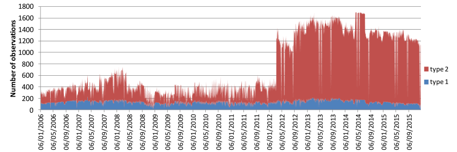
Note: Securitisation types in the table are our approximations to the types in Solvency II. Due to data limitations, our Type 1 criteria are only necessary conditions of Solvency II requirements. Thus our Type 1 securitisations may have included some Type 2 securitisations under Solvency II. The total number of observations surges in March 2012 when BVAL was launched by Bloomberg.
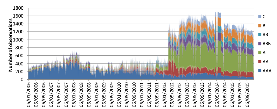
Note: Daily ratings of each bond are inferred from rating transitions issued by S&P, Moody’s and Fitch. Rating transition data is obtained from Thomson Reuters Eikon. The total number of observations surges in March 2012 when BVAL was launched by Bloomberg.
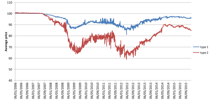
Note: Securitisation types in the figure are our approximations to the types in Solvency II. Price discounts before March 16th 2012 are scaled up to compensate for any unobserved risky positions before the launch of BVAL.
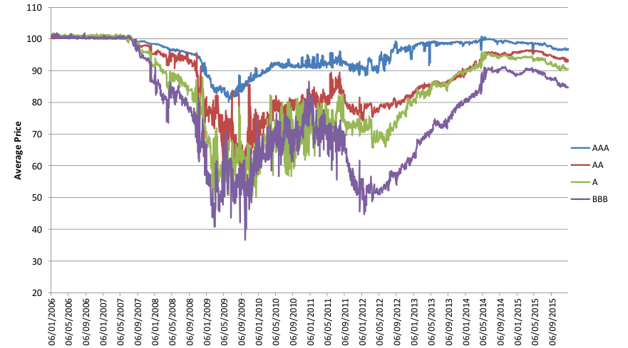
Note: Price discounts before March 16th 2012 are scaled to compensate for any unobserved risky positions before the launch of BVAL.
3.4. VaR Methodology and Results
We calculate one year 99.5% value at risk (VaR) using bootstrapping methods.[17] For each securitisation category (i.e. a securitisation type or a rating category), we randomly bootstrap 52 samples from the category’s historical index and calculate their mean value as one simulated yearly return. We repeat this calculation 100,000 times, and sort the simulated returns from lowest to highest. The 99.5% VaR is the negative of the 500th (100,000 × 0.5% ) lowest simulated return.
On a given day, the average return per modified duration of a certain category incorporates high idiosyncratic risk if there are too few observations in this category. Therefore for each category, we only sample from the index elements with no less than 10 corresponding observations. For type indices, we do not lose any sample since the numbers of observations of both types on each day are more than 10. However, in bootstrapping ratings, we lose some index elements of AA, A and BBB ratings. The rating bootstrapping sample sizes within each calendar year are presented in Table 8.[18]
Note that there are very few observations of daily prices of BB and C rating bonds before 2011, and very few observations of B-rated bonds before the data boost in
2012. Attempts to simulate returns for B-rated bonds will, therefore, omit observations corresponding to the 2007-2009 financial crisis. For this reason, we only attempt to estimate VaRs for bonds rated no lower than BBB.
We conduct simulations on non-overlapping windows only.[19] To generate nonoverlapping indices for bootstrapping, the following steps are taken. First, days with no price data are deleted. Second, for each day in our sample, we calculate an average return per modified year of duration for the following 5 working-day windows. If, on a given day, there are fewer than 35 bonds of all categories with a return over the next week, that day is deleted. Third, for each given factor category, we choose dates with more than 10 bond return observations in that category. Fourth, we choose the 1st, 6th, 11th, etc element of each index as the sample for bootstrapping.
The VaR results obtained from simulating yearly returns as just described are displayed in Table 9.
We infer the VaRs in each type-rating sub-category by two calibrations. Calibration 1 adopts an extremely conservative approach which takes the calibrated rating VaRs as VaRs for Type 1 ratings. The VaRs for Type 2 ratings are inferred by the ratio of Type 2 VaR and Type 1 VaR. For a given Type i and rating r, Calibration 1 calculates its VaR by equation (8).
VaRi,r = {VaRr , i= Type 1, r= AAA, AA, A, BBB VaRr × (VaRType2/VaRType1) , i= Type 2, r= AAA, AA, A, BBB(8)
Calibration 2 follows a less conservative approach as illustrated in equation (9). Calibration 2 still maintain the ratio between Type 1 and Type 2 capital, but tackles the rating VaRs as the geometric mean of the VaRs of the Type 1 and Type 2 bonds with this rating. Note that the Calibration 2 is still conservative; each rating category actually has considerably more Type 2 securitisations than Type 1 securitisations. Consequently, the rating VaRs should be close to the Type 2 rating VaRs. Thus Calibration 2 is still likely to overestimate VaRs for each sub-category.
VaRr/√VaRType2/VaRType1 , i= Type 1, r= AAA, AA, A, BBB VaRi,r = { VaRr × √VaRType2/VaRType1 , i= Type 2, r= AAA, AA, A, BBB (9)
The inferred VaRs of all sub-categories are shown in Table 10. For Type 1 bonds, our results for AAA, AA and A rating bonds are all lower than Solvency II capital ratios. Our Type 1 BBB capitals are higher than the 3% capital requirement in Solvency II. All our results for Type 2 securitisations are much lower than Solvency II capital ratios.
For comparison purposes, we also show in Table 10 the Solvency II per-year-ofduration capital charges for securitisations and for different spread-module asset classes, namely corporate bonds and covered bonds. The most striking comparison is between our Calibration 2 results for Type 1 securitisation and the corporate bonds charges which are very similar. Covered bonds attract noticeably lower charges than our Calibration 2 results.
It is worthy of mention that our sample contains distinctly fewer AA and BBB rated bonds compared to those that are rated AAA and A (see Figure 2). The average number of daily observations for bonds rated AAA, AA, A and BBB (after deleting days with fewer than 10 observations for each rating category) are 191, 85, 220, and 86, respectively. The smaller samples for AA and BBB rated bonds may lead to overestimation of the VaRs for these categories.
Note that the higher volatility and, hence, VaR estimates for A and BBB rated tranches may well reflect their lower liquidity in the market. Bonds in these rating ranges include both senior tranches that have been downgraded (which offer reasonable liquidity) and third-to-pay and below tranches (which are often illiquid). Liquidity premia fluctuated considerably in the crisis leading to marked price volatility especially for this latter category of exposure.
| AAA | AA | A | BBB | |
|---|---|---|---|---|
| 2006 | 248 | 167 | 236 | 218 |
| 2007 | 253 | 181 | 236 | 227 |
| 2008 | 253 | 193 | 228 | 208 |
| 2009 | 254 | 204 | 234 | 140 |
| 2010 | 256 | 254 | 250 | 153 |
| 2011 | 256 | 256 | 255 | 212 |
| 2012 | 256 | 256 | 256 | 253 |
| 2013 | 256 | 256 | 256 | 256 |
| 2014 | 252 | 252 | 252 | 252 |
| 2015 | 254 | 254 | 252 | 252 |
| Total | 2538 | 2273 | 2455 | 2171 |
Note: For the return index of a given rating, days with fewer than 10 observations are removed from the bootstrap sample. We do not discuss ratings lower than BBB as they lack observations during the 2007-2009 financial crisis.
| 99.5% | VaR |
|---|---|
| Type 1 | 1.69 |
| Type 2 | 3.29 |
| AAA | 1.27 |
| AA | 1.59 |
| A | 1.98 |
| BBB | 7.11 |
Note: The simulation results are based on non-overlapping windows and are given in percent.
| Calibration | 1 Calibration | 2 | Securitisations Corporate | Bonds Covered | Bonds | ||
|---|---|---|---|---|---|---|---|
| Type | 1 | AAA | 1.27 | 0.91 | 2.1 | 0.9 | 0.7 |
| Type | 1 | AA | 1.59 | 1.14 | 3 | 1.1 | 0.9 |
| Type | 1 | A | 1.98 | 1.42 | 3 | 1.4 | - |
| Type | 1 | BBB | 7.11 | 5.10 | 3 | 2.5 | - |
| Type | 2 | AAA | 2.47 | 1.77 | 12.5 | - | - |
| Type | 2 | AA | 3.10 | 2.22 | 13.4 | - | - |
| Type | 2 | A | 3.85 | 2.76 | 16.6 | - | - |
| Type | 2 | BBB | 13.84 | 9.92 | 19.7 | - | - |
Note: The annual VaRs are shown in percent for each type/rating pair. Calibration 1 is extremely conservative and Calibration 2 is moderately conservative. The Solvency II capital charges for securitisations, corporate bonds and covered bonds are provided for comparison. The capital charges for corporate bonds and covered bonds actually scale more slowly when the modified duration is greater than 5 years.
4. Capital calibration
4.1. Representative insurer
In implementing the Solvency II capital charges, we present results with and without diversification adjustments. Such adjustments depend on the composition of the insurer’s portfolio. In our case, we derive adjustments appropriate for the representative European life insurer described in Höring (2012). This insurer has total assets of EUR 4 billion. Its market risk portfolio has a total value of EUR 3 billion. Table 11 shows a breakdown of the market risk portfolio.
Calculating the capital requirement for the spread risk sub-module requires that one know the modified duration of each exposure. We assume, for simplicity, that exposures in each asset class have a single representative duration. The representative durations we employ are shown in Table 12.
The asset and liability durations for Höring’s representative insurer are assumed to be 6.8 and 8.9 years, respectively. To calculate capital for the interest rate risk sub-module, an average downward interest rate shock is calculated using the
March 2016 risk free curves provided by EIOPA. This is multiplied by the difference of 2.1 between the liability and asset durations and the result is multiplied by the asset total of EUR 4 billion.
According to the fifth quantitative impact study for Solvency II (QIS5), the total capital requirement for the remaining risk modules is much lower than the capital requirement for the market risk module. Table 13 reproduces data contained in Graph 32 of QIS5 consisting of the average diversified capital charges for each risk module as a percentage of the Basic Solvency Capital Requirement (BSCR).
In order to calculate capital requirements for the remaining risk modules, we assume that the capital charges of the representative European life insurer have the same break-down.[20]
| Sub-module | Subtype | AAA | AA | A | BBB | BB | ≤B | Unrated | Total |
|---|---|---|---|---|---|---|---|---|---|
| Type 1 | - | - | - | - | - | - | - | 4.5 | |
| Equity | |||||||||
| Type 2 | - | - | - | - | - | - | - | 2.5 | |
| Property | - | - | - | - | - | - | - | 11.0 | |
| Bonds | 5.2 | 4.4 | 11.8 | 5.9 | 0.6 | 0.1 | 1.5 | 29.5 | |
| Covered bonds | 11.5 | 0.5 | 0.3 | 0.1 | - | - | 0.1 | 12.5 | |
| Spread | |||||||||
| Sovereign debt (EEA) | 18.8 | 6.6 | 5.8 | 0.2 | 0.6 | - | - | 32.0 | |
| Sovereign debt (Non-EEA) | 5.2 | 1.4 | 0.2 | 0.8 | - | 0.2 | 0.2 | 8.0 |
Note: The market risk portfolio of a representative European-based life insurer is shown broken down by Solvency II sub-module, and further broken down by the subtypes considered in each sub-module and the credit rating of exposures considered in the spread risk sub-module. The entries are given as a percentage of the total EUR 3 billion value of the market risk portfolio.
| Asset class Modified | duration |
|---|---|
| Bonds | 5.4 |
| Covered bonds | 6.2 |
| Sovereign debt | 6.9 |
Note: These values show the average modified duration of exposures to different asset classes treated under the market risk module for a representative European-based life insurer. The values are provided in Höring (2012).

Note: These values are provided in Graph 32 of QIS5. They show the average diversified capital requirement for the market risk module as a percentage of the Basic Solvency Capital Requirement.
4.2. Capital calculations
This section presents the impact of different capital rules on (i) a set of representative securitisation exposures and (ii) 1,705 European securitisations exposures for which we have comprehensive information. Looking at (ii) shows how rules affect the European market as it currently exists. However, the composition of the sample employed necessarily affects the results. So it is helpful also to consider the effects on representative bonds as in (i).
The 1,705 securitisation tranches in (ii) are a different sample from that employed (numbering 8,322) in the VaR estimation described above. Hence, we restrict attention to those for which we could estimate pool default probabilities (based on Intex data) required as inputs by the SEC-IRBA approach.
Solvency II capital charges are presented using the current calibration (see Table 5) and the alternative calibrations proposed in Section 3.4. Using our model of a representative insurer, we calculate Solvency II capital for an individual exposure by subtracting the insurer’s total Solvency II capital requirement from the Solvency II capital assuming the insurer holds its original portfolio plus the exposure in question. We also present, for comparison purposes the capital charges implied by the Basel III rules specified in BCBS 303.
Capital Requirement (SCR) is calculated from the BSCR by multiplying by the factor: 0.674. This factor is obtained from Graph 34 of QIS5.
Finally, we calculate “bottom up” capital charges for the securitisation exposures and Basel III capital calculations by way of comparison. The bottom up capital estimates are generated by calculating the Solvency II capital charge for the underlying pool assets and then using it as an input to the Simplified Supervisory Formula Approach (SSFA) of the Basel III rules (see, for example, BCBS 269).[21]
Note that in these bottom up calculations, the pool asset capital is calculated inclusive of a diversification adjustment in the sense that it is based on the difference between the Solvency II capital of a portfolio inclusive of the pool assets minus the Solvency II capital without the pool assets.[22]
We start by considering capital charges for a set of representative securitisations. EBA (2014) follows a similar approach of looking at the impact of capital rules on representative securitisations. In our case, however, we employ actual rather than stylised transactions. The bonds we consider are shown in Table 14.
Table 15 shows the capital charges implied by the rules exposited above for the bonds listed in Table 14. Several points are deserving of mention.
First, the diversification adjustment significantly reduces the capital charge implied by the Solvency II approach under the different calibrations. This is clearly appropriate given that almost no insurer will hold substantial amounts of securitisation exposures relative to their other asset holdings. We do not analyse, in this study, the appropriateness of the diversification adjustment. It has been questioned by some authors (see Pfeifer and Strassburger (2008) and Floreani (2012)).[23]
Second, it is noticeable that the Calibration 2 variant of the Solvency II approach (which is already conservative as noted in Section 3) implies capital charges for the representative exposures that are about half the size of those obtained using the current Solvency II calibration. This is true either before or after diversification adjustment.
Third, with the exception of auto loan backed securitisations, the Solvency II capital charges based on the Calibration 2 variant are still substantially higher than those implied by the Basel III approaches.
Fourth, the bottom up calculation of capital yields results that are lower than other approaches including the Basel III approaches that also use the SSFA. This reflects the paradoxical aspect of the Solvency II calibration more generally that bank loans directly held by an insurer are regarded as less risky than if they are held by a bank, whereas securitisations, which provide senior claims on pools of bank loans, are viewed as more risky when held by an insurer than by a bank.[24]
Another way to compare the impact of different capital charges is to examine the average percentage capital charges they imply for sets of securitisation positions. Tables 16-19 display simple unweighted averages of capital charges for different subsets of an extensive sample of 1,705 European securitisation exposures.
The sample studied in Tables 16-19 is the same as that employed in several past studies of the Basel III capital rules, including Duponcheele, Linden and Perraudin (2014) and (2015),[25] and we thank the authors of those papers for allowing us to use those data. We have collected additional data including making estimates of the Weighted Average Lives of the securitisation tranches included in the sample in order to perform the analysis in this paper.
In the successive Tables 16 to 19, we look at average capital charges broken down by country (Table 16), asset class (Table 17), rating (Table 18) and modified duration (Table 19). In interpreting the results, it is important to allow for the fact that, when one compares the results from two subsets, for example Type 1 and
Type 2, the subsets of securities also differ in other respects. This accounts for some apparently anomalous results.
For example, in Table 18, for one calibration, the AAA-rated Type 1 tranches have a higher average capital charge than their Type 2 equivalents. This higher average capital charge results from the relatively short durations of the Type 2 exposures in the sample (of which, in any case, there are only 8).
One may see from Table 16 that the largest sets of transactions are for Spain and the UK (see the right hand column). German, Spanish and Portuguese exposures attract the highest Solvency II capital. The results under the 2nd calibration variant are in many cases again about half the capital charges implied by the current Solvency II rules. Exceptions are Spain and Portugal. This latter finding reflects the fact that, for BBB-rated Type 1 positions, the two variant calibrations are conservative relative to the current Solvency II rules.
The asset class breakdown shown in Table 17 suggests that, in the case of Type 1 exposures, the relative conservatism of the Solvency II approach relative to the Basel III rules is driven by high capital charges for RMBS and, to some extent for SME-backed deals. This is striking given that, in the recent crisis, these two asset classes exhibited vanishingly small delinquency rates despite the severity of the macroeconomic shocks experienced.
The results shown in Table 17 show that Type 2 exposures attract capital under the ERBA that is just half of that implied by Solvency II. But, if a bank can use the IRBA, its capital can be no more than a tenth of that prescribed by Solvency II. This underlines the incoherence of the Basel III approaches, a point emphasised in Duponcheele, Linden and Perraudin (2014) and (2015).
Table 18 shows results for exposures categorised by credit rating. As one might expect from the raw per-year-of-duration capital charges (see Table 5), there is not much of a progression between rating grades AA and BBB in the results based on the current Solvency II rules. Both the alternative variant calibrations and the Basel III External Ratings Based Approach (ERBA) show considerably more progression across these rating grades.
Note that the nature of the sample is very important in explaining individual results. For example, in Table 18, the Solvency II capital charges without diversification adjustment for AAA Type 2 are 21%. This reflects the fact that there are only eight such bonds and the average duration is about 2 years.
Finally, Table 19 shows results broken down by durations. The results in Table 19 show that Solvency II is less conservative relative to the Basel III rules for short duration transactions than it is for long duration bonds. In the latter case, for Type 1 bonds, the ratio of Basel III to Solvency II capital can exceed 40. (One should recall that the Basel III rules applied in these calculations are of BCBS 303 which many European regulators have regarded as excessively conservative for high quality European securitisation tranches.)
| Asset Class | Country | ISIN | Rating | Dur. AP | (%) DP | (%) | Delin. PD | (%) | LGD |
|---|---|---|---|---|---|---|---|---|---|
| (years) | (%) | (%) | |||||||
| Type 1 | |||||||||
| GB | XS0744002139 | AAA | 7.1 | 32.0 | 100.0 | 1.4 | 1.5 | 15 | |
| RMBS | Spain | ES0312273289 | A- | 7.4 | 16.7 | 100.0 | 0.2 | 2.0 | 15 |
| Portugal | XS0293657416 | A- | 12.4 | 6.3 | 100.0 | 1.1 | 2.0 | 20 | |
| GB | XS0608382593 | AAA | 3.0 | 56.8 | 100.0 | 0.0 | 2.0 | 30 | |
| SME | |||||||||
| Spain | ES0357326000 | AA- | 4.0 | 41.6 | 100.0 | 8.5 | 5.0 | 35 | |
| Germany | XS0782698988 | AAA | 0.7 | 19.9 | 100.0 | 0.0 | 0.8 | 40 | |
| Auto loans | GB | XS0852485456 | AAA | 0.7 | 35.4 | 100.0 | 0.2 | 0.8 | 40 |
| Spain | ES0327055002 | AA- | 0.5 | 32.0 | 100.0 | 0.0 | 1.0 | 40 | |
| Con. loans | GB | XS0219226841 | AA | 6.1 | 78.2 | 100.0 | 10.1 | 17.1 | 40 |
| Type 2 | |||||||||
| Asset Class | Country | ISIN | Rating | Dur. AP | (%) DP | (%) | Delin. PD | (%) | LGD |
| GB | XS0246904238 | A | 10.3 | 14.6 | 28.0 | 0.0 | 1.0 | 15 | |
| RMBS | Spain | ES0312371018 | A- | 10.1 | 22.4 | 62.7 | 8.2 | 6.0 | 15 |
| Portugal | XS0177083259 | A- | 12.8 | 19.7 | 31.9 | 2.5 | 2.0 | 20 | |
| GB | XS0845530939 | A+ | 9.8 | 31.2 | 45.9 | 0.0 | 2.0 | 30 | |
| SME | |||||||||
| Spain | ES0338048038 | BBB | 8.4 | 27.9 | 49.5 | 0.0 | 5.0 | 35 | |
| Germany | XS0644547498 | AA- | 1.0 | 13.0 | 25.1 | 0.0 | 0.8 | 40 | |
| Auto loans | GB | XS0852486264 | A+ | 1.7 | 18.8 | 35.4 | 0.2 | 0.8 | 40 |
| Spain | ES0307769028 | A- | 1.4 | 55.7 | 86.8 | 2.4 | 1.8 | 40 | |
| Con. loans | GB | XS0219230017 | A | 7.1 | 45.9 | 62.0 | 10.1 | 17.1 | 40 |
Note: The rating and duration of the representative exposures are the only values affecting their Solvency II capital charges. The last five columns show the attachment point, detachment point, delinquencies, probability of default and loss given default. Probability of default and loss given default are defined in BCBS 128. The PD figures provided are estimated using Intex data using the methodology described in Duponcheele, Linden and Perraudin (2014). The LGDs are derived using the approach described in Duponcheele, Linden, Perraudin and Totouom-Tangho (2014).
| Solvency II | capital | charge | Solvency II | capital | charge | ||||||
|---|---|---|---|---|---|---|---|---|---|---|---|
| Basel | III capital | charge (%) | |||||||||
| without | diversification | (%) | with | diversification | (%) | ||||||
| Asset Class | Country SII | cal. | 1st cal. | 2nd cal. SII | 1st cal. | 2nd cal. | cal. | IRBA | ERBA | SA SSFA | SII |
| Type 1 | |||||||||||
| GB | 14.9 | 9.0 | 6.4 | 8.7 | 5.2 | 3.8 | 1.2 | 1.6 | 1.2 | 1.2 | |
| RMBS | Spain | 22.1 | 14.6 | 10.5 | 13.3 | 8.7 | 6.2 | 1.2 | 5.6 | 1.2 | 1.2 |
| Portugal | 37.3 | 24.6 | 17.6 | 22.4 | 14.6 | 10.4 | 1.5 | 5.6 | 1.4 | 3.3 | |
| GB | 6.3 | 3.8 | 2.7 | 3.6 | 2.2 | 1.6 | 1.2 | 3.2 | 1.2 | 1.2 | |
| SME | |||||||||||
| Spain | 12.1 | 6.4 | 4.6 | 7.0 | 3.7 | 2.7 | 1.2 | 3.6 | 1.2 | 1.2 | |
| Germany | 2.1 | 1.3 | 0.9 | 1.2 | 0.8 | 0.6 | 1.2 | 1.6 | 1.2 | 1.2 | |
| Auto loans | GB | 2.1 | 1.3 | 0.9 | 1.2 | 0.8 | 0.6 | 1.2 | 1.5 | 1.2 | 1.2 |
| Spain | 3.0 | 1.6 | 1.1 | 1.8 | 1.0 | 0.7 | 1.2 | 5.6 | 1.2 | 1.2 | |
| Con. loans | GB | 18.4 | 9.8 | 7.0 | 10.5 | 5.6 | 4.0 | 1.2 | 3.2 | 1.2 | 1.2 |
| Type 2 | |||||||||||
| GB | 100.0 | 39.7 | 28.5 | 57.4 | 22.7 | 16.2 | 1.2 | 12.5 | 1.2 | 1.2 | |
| RMBS | Spain | 100.0 | 39.0 | 28.0 | 57.9 | 22.4 | 16.0 | 1.2 | 10.0 | 1.6 | 2.1 |
| Portugal | 100.0 | 49.1 | 35.2 | 57.4 | 28.1 | 20.1 | 1.2 | 14.7 | 1.2 | 1.2 | |
| GB | 100.0 | 37.7 | 27.0 | 61.6 | 22.4 | 15.9 | 1.2 | 10.9 | 1.2 | 16.6 | |
| SME | |||||||||||
| Spain | 100.0 | 100.0 | 83.4 | 58.7 | 58.7 | 48.7 | 1.2 | 19.5 | 1.2 | 12.2 | |
| Germany | 13.4 | 3.1 | 2.2 | 7.7 | 1.8 | 1.3 | 1.5 | 8.4 | 13.3 | 1.2 | |
| Auto loans | GB | 28.6 | 6.6 | 4.8 | 16.3 | 3.8 | 2.7 | 1.2 | 9.2 | 4.2 | 1.2 |
| Spain | 22.9 | 5.3 | 3.8 | 13.2 | 3.1 | 2.2 | 1.2 | 11.6 | 1.2 | 1.2 | |
| Con. loans | GB | 100.0 | 27.2 | 19.5 | 57.2 | 15.5 | 11.1 | 1.2 | 12.1 | 1.7 | 7.0 |
Note: Capital charges are shown for a set of representative securitisation exposures with varying asset class and country of issuance. Further information about these exposures is given in Table 14.
| Solvency II | capital | charge | Solvency II | capital | charge | ||||||
|---|---|---|---|---|---|---|---|---|---|---|---|
| Basel | III capital | charge | (%) | ||||||||
| without | diversification | (%) with | diversification | (%) | |||||||
| SSFA No. | of | ||||||||||
| Country SII | cal. 1st | cal. | 2nd SII cal. | cal. 1st | 2nd cal. | cal. | IRBA | ERBA | SA | SII | exp. |
| Type 1 | |||||||||||
| Germany | 29.7 | 18.4 | 13.2 | 19.1 | 11.7 | 8.3 | 1.2 | 2.2 | 1.7 | 3.3 | 31 |
| Great Britain | 8.3 | 4.9 | 3.5 | 5.0 | 2.9 | 2.1 | 1.2 | 2.0 | 1.2 | 1.3 | 160 |
| Italy | 14.8 | 9.5 | 6.8 | 9.1 | 5.8 | 4.1 | 1.2 | 5.2 | 1.2 | 1.2 | 30 |
| Netherlands | 7.7 | 4.7 | 3.3 | 4.7 | 2.8 | 2.0 | 1.3 | 2.1 | 1.4 | 3.7 | 87 |
| Portugal | 31.4 | 34.0 | 24.3 | 19.9 | 21.6 | 15.3 | 1.3 | 7.1 | 1.4 | 2.1 | 25 |
| Spain | 18.4 | 28.0 | 20.1 | 11.3 | 17.5 | 12.4 | 1.2 | 6.5 | 1.3 | 2.7 | 181 |
| Type 2 | |||||||||||
| Germany | 67.6 | 60.2 | 59.1 | 39.7 | 35.4 | 34.8 | 22.9 | 35.9 | 30.7 | 28.1 | 47 |
| Great Britain | 58.3 | 32.8 | 27.7 | 34.4 | 19.3 | 16.2 | 2.8 | 12.2 | 6.9 | 10.3 | 121 |
| Italy | 78.9 | 34.2 | 28.4 | 49.3 | 20.8 | 17.2 | 4.5 | 12.2 | 11.4 | 14.6 | 122 |
| Netherlands | 65.1 | 50.5 | 46.8 | 38.3 | 29.9 | 27.7 | 22.6 | 28.6 | 37.4 | 44.5 | 131 |
| Portugal | 97.6 | 81.2 | 77.6 | 60.4 | 50.0 | 47.8 | 12.6 | 27.4 | 17.3 | 20.5 | 79 |
| Spain | 89.8 | 80.9 | 73.7 | 55.7 | 50.1 | 45.5 | 10.0 | 31.5 | 18.3 | 21.3 | 605 |
Note: Capital charges are shown for all 1705 securitisation exposures, with the exposures grouped by country of issuance. The least populated countries are not shown. For Type 1 Portuguese and Spanish exposures the capital charges under both the 1st and 2nd calibration are higher than the capital charge under the Solvency II calibration. This is due to the large number of BBB-rated Portuguese and Spanish securitisation exposures in our dataset.
| Solvency II | capital | charge | Solvency II | capital | charge | ||||||
|---|---|---|---|---|---|---|---|---|---|---|---|
| Basel | III capital | charge | (%) | ||||||||
| without | diversification | (%) with | diversification | (%) | |||||||
| SSFA No. | of | ||||||||||
| Asset class SII | cal. 1st | cal. | 2nd SII cal. | cal. 1st | 2nd cal. | cal. | IRBA | ERBA | SA | ||
| SII | exp. | ||||||||||
| Type 1 | |||||||||||
| Auto loans | 3.0 | 1.8 | 1.3 | 1.8 | 1.1 | 0.8 | 1.2 | 2.0 | 1.8 | 1.2 | 43 |
| & leases | |||||||||||
| Con. loans | 5.2 | 3.4 | 2.4 | 3.1 | 2.0 | 1.4 | 1.2 | 3.7 | 1.2 | 1.2 | 12 |
| RMBS | 14.8 | 14.7 | 10.5 | 9.2 | 9.1 | 6.5 | 1.2 | 3.8 | 1.3 | 2.4 | 423 |
| SME | 6.2 | 5.9 | 4.3 | 3.6 | 3.5 | 2.5 | 1.2 | 4.8 | 1.3 | 1.6 | 50 |
| Type 2 | |||||||||||
| Auto loans | 22.2 | 6.3 | 4.9 | 13.1 | 3.7 | 2.8 | 3.6 | 8.3 | 12.5 | 6.9 | 36 |
| & leases | |||||||||||
| Con. loans | 71.7 | 53.0 | 48.4 | 43.0 | 31.8 | 29.0 | 6.9 | 29.1 | 18.9 | 21.8 | 34 |
| RMBS | 88.9 | 71.5 | 65.4 | 55.4 | 44.4 | 40.5 | 8.9 | 25.9 | 14.7 | 18.1 | 936 |
| SME | 67.1 | 56.8 | 54.0 | 39.7 | 33.6 | 31.9 | 11.4 | 33.2 | 23.0 | 23.9 | 171 |
Note: Capital charges are shown for all 1705 securitisation exposures, with the exposures grouped by asset class. The Solvency II capital charges are particularly high compared to the Basel III capital charges for RMBS, where the modified duration is high.
| Solvency II | capital | charge | Solvency II | capital | charge | ||||||
|---|---|---|---|---|---|---|---|---|---|---|---|
| Basel | III capital | charge | (%) | ||||||||
| without | diversification | (%) with | diversification | (%) | |||||||
| SSFA No. | of | ||||||||||
| Rating SII | cal. | 1st cal. | 2nd SII cal. | cal. 1st | 2nd cal. | cal. | IRBA | ERBA | SA | ||
| SII | exp. | ||||||||||
| Type 1 | |||||||||||
| AAA | 9.0 | 5.4 | 3.9 | 5.6 | 3.3 | 2.4 | 1.2 | 1.6 | 1.3 | 2.1 | 201 |
| AA | 16.9 | 8.9 | 6.4 | 10.4 | 5.5 | 3.9 | 1.2 | 3.4 | 1.3 | 2.6 | 68 |
| A | 19.3 | 12.7 | 9.1 | 11.9 | 7.8 | 5.5 | 1.3 | 5.6 | 1.4 | 1.9 | 183 |
| BBB | 19.9 | 47.1 | 33.8 | 12.2 | 29.7 | 21.1 | 1.2 | 8.7 | 1.3 | 3.0 | 76 |
| Type 2 | |||||||||||
| AAA | 21.0 | 4.2 | 3.0 | 12.6 | 2.4 | 1.8 | 1.2 | 3.0 | 3.0 | 3.4 | 8 |
| AA | 64.7 | 18.4 | 13.2 | 40.5 | 11.2 | 7.9 | 2.0 | 6.3 | 6.1 | 9.1 | 113 |
| A | 71.2 | 25.7 | 18.8 | 43.6 | 15.4 | 11.1 | 2.8 | 9.0 | 8.5 | 10.1 | 229 |
| BBB | 84.8 | 73.5 | 59.9 | 53.2 | 45.9 | 37.1 | 4.1 | 16.0 | 10.4 | 14.0 | 225 |
| BB | 99.2 | 99.2 | 99.2 | 61.8 | 61.8 | 61.8 | 5.9 | 30.3 | 12.2 | 15.4 | 199 |
| B | 100.0 | 100.0 | 100.0 | 62.3 | 62.3 | 62.3 | 11.4 | 45.0 | 20.5 | 23.9 | 183 |
| <B | 100.0 | 100.0 | 100.0 | 60.1 | 60.1 | 60.1 | 47.3 | 81.0 | 55.6 | 58.7 | 220 |
Note: Capital charges are shown for all 1705 securitisation exposures, with the exposures grouped by credit rating. The Solvency II capital charges for Type 1 AAA rated securitisation exposures are higher than those for Type 2 AAA rated exposures when either of the calibrations derived in Section 3 are used, reflecting the low duration of the small number of Type 2 AAA rated exposures.
| Solvency II | capital | charge | Solvency II | capital | charge | |||||||||
|---|---|---|---|---|---|---|---|---|---|---|---|---|---|---|
| Basel | III capital | charge | (%) | |||||||||||
| without | diversification | (%) with | diversification | (%) | ||||||||||
| Duration | SSFA No. | of | ||||||||||||
| SII | cal. 1st | cal. | 2nd SII cal. | cal. 1st | cal. | 2nd | cal. | IRBA | ERBA | SA | ||||
| (years) | SII | exp. | ||||||||||||
| Type | 1 | |||||||||||||
| 0 ≤ dur < | 5 | 4.5 | 3.4 | 2.4 | 2.7 | 2.0 | 1.5 | 1.2 | 2.8 | 1.3 | 2.0 | 358 | ||
| 5 ≤ dur < | 10 | 20.4 | 25.6 | 18.3 | 12.4 | 15.9 | 11.3 | 1.2 | 5.4 | 1.2 | 2.4 | 136 | ||
| 10 ≤ dur | < | 15 | 34.5 | 32.3 | 23.1 | 21.9 | 20.5 | 14.6 | 1.3 | 5.0 | 1.3 | 2.3 | 19 | |
| 15 ≤ dur | < | 20 | 48.2 | 31.3 | 22.5 | 30.2 | 19.2 | 13.7 | 1.2 | 4.1 | 1.2 | 2.9 | 11 | |
| 20 ≤ dur | 56.7 | 34.2 | 24.5 | 36.8 | 21.9 | 15.6 | 1.2 | 1.6 | 1.2 | 6.3 | 4 | |||
| Type | 2 | |||||||||||||
| 0 ≤ dur < | 5 | 57.0 | 37.5 | 33.1 | 34.8 | 22.8 | 20.1 | 4.1 | 17.8 | 10.2 | 10.5 | 434 | ||
| 5 ≤ dur < | 10 | 99.2 | 79.4 | 70.7 | 62.9 | 50.1 | 44.5 | 4.0 | 20.7 | 8.8 | 12.2 | 239 | ||
| 10 ≤ dur | < | 15 | 100.0 | 86.4 | 83.3 | 61.7 | 53.3 | 51.3 | 9.2 | 27.3 | 16.4 | 21.2 | 222 | |
| 15 ≤ dur | < | 20 | 100.0 | 94.4 | 91.6 | 59.5 | 56.0 | 54.3 | 31.8 | 59.8 | 43.3 | 49.6 | 154 | |
| 20 ≤ dur | 100.0 | 99.0 | 97.1 | 60.1 | 59.5 | 58.3 | 45.0 | 72.2 | 57.4 | 64.4 | 128 |
Note: Capital charges are shown for all 1705 securitisation exposures, with the exposures grouped by modified duration. The Solvency II capital charges exhibit a strong correlation to their modified duration. This follows from the fact that the capital charge formula is proportional to modified duration.
5. Conclusion
This paper analyses the calibration of capital charges for securitisation exposures within the European Solvency II framework. The Solvency II framework is based on per-year-of-duration capital charges broken down by rating and distinguishing between Type 1 and 2 securitisation tranches. (The Type 1 category is designed to identify exposures that are likely to exhibit lower risk for a given rating and duration.)
The European authorities have made several attempts to devise a satisfactory calibration using a variety of approaches. The latest version has several counterintuitive features including no differentiation between capital charges for Type 1 tranches rated below AAA and implausibly large gaps between the charges for Type 1 and Type 2 tranches.
Here, we estimate per-year-of-duration charges for tranches broken down by rating and type. In so doing, we employ securitisation indices, running from before the crisis to January 2016, that we construct ourselves from security-level market price data. Our approach yields indices that are directly reflective of the categories of securitisation in which we are interested. (This is not possible using publicly available index data.)
We also perform a calibration of securitisation capital using a “look through” or “bottom up” approach in which we calculate capital charges for underlying securitisation pools and then apply the Simplified Supervisory Formula Approach (SSFA) of the Basel III rules to divide this pool capital between different tranches in a given deal, based on their attachment and detachment points and cumulated pool delinquencies.
Our findings are that AAA-rated Type 1 and Type 2 in general are much too conservatively treated under current Solvency II rules. A conservative variant of our alternative calibration (the other variant we consider is very conservative) implies capital charges for these categories that are about half those currently applied within Solvency II. The charges implied by our analysis for Type 1 securitisations are quite similar to the Solvency II charges for corporate bonds. Our bottom up calibration implies lower capital still.[26]
In summary, our analysis provides strong arguments for a review of Solvency II capital charges for securitisations. The charges for highly rated Type 1 tranches and all Type 2 tranches merit reconsideration.
References
1. Arias, Liliana, Mohamed El Hedi Arouri, Philippe Foulquier and Stéphane Gregoir (2010) “On the Suitability of the Calibration of Private Equity Risk in the Solvency II Standard Formula,” EDHEC Business School mimeo, April, available at:http://faculty-research.edhec.com/research/edhecpublications/2010/solvency-ii-on-the-suitability-of-the-calibration-of-privateequity-risk-in-the-solvency-ii-standard-formula-141279.kjsp
2. Association for Financial Markets in Europe (2011) “Report for the European Commission on the Capital Charge Treatment of Asset Backed Securities under Solvency II Standard SCR,” July
3. Bank of England and European Central Bank (2014a) “The Impaired EU Securitisation Market: Causes, Roadblocks and How to Deal With Them,” Bank of England and European Central Bank Joint Statement, April, available at: http://www.bankofengland.co.uk/publications/Pages/news/2014/070.aspx
4. Bank of England and European Central Bank (2014b) “The Case for a Better Functioning Securitisation Market in the European Union: A Discussion Paper,” Bank of England and European Central Bank Joint Publication, May, available at: https://www.ecb.europa.eu/pub/pdf/other/ecbboe_case_better_functioning_securitisation_marketen.pdf
5. Basel Committee on Banking Supervision (2006) “International Convergence of Capital Measurement and Capital Standards,” Bank for International Settlements, June, (also known as BCBS 128), available at:http://www.bis.org/publ/bcbs128.htm
6. Basel Committee on Banking Supervision (2012) “Revisions to the Basel Securitisation Framework,” Consultative Document, Bank for International
Settlements, December, (also known as BCBS 236), available at: http://www.bis.org/publ/bcbs236.pdf
7. Basel Committee on Banking Supervision (2013) “Revisions to the securitisation framework,” Consultative Document, Bank for International Settlements, December, (also known as BCBS 269), available at: http://www.bis.org/publ/bcbs269.pdf
8. Basel Committee on Banking Supervision (2014) “Revisions to the securitisation framework,” Basel III document, Bank for International Settlements, December, (also known as BCBS 303), available at: http://www.bis.org/bcbs/publ/d303.htm
9. Committee of European Insurance and Occupational Pensions Supervisors
(2010) “CEIOPS’ Advice for Level 2 Implementing Measures on Solvency II: SCR Standard Formula Article 111b Calibration of Market Risk Module,” January, (also known as CEIOPS-DOC-66/10), available at: https://eiopa.europa.eu/CEIOPS-Archive/Documents/Advices/CEIOPS-L2- Advice-Market-risk-calibration.pdf
10. Duponcheele, Georges, William Perraudin and Daniel Totouom-Tangho
(2013a) “A Principles-Based Approach to Regulatory Capital for Securitisations,” BNP Paribas mimeo, April, available at: http://www.riskcontrollimited.com/insights/a-principles-based-approach-toregulatory-capital-for-securitisations/
11. Duponcheele, Georges, William Perraudin and Daniel Totouom-Tangho
(2013b) “Maturity Effects in Securitisation Capital: Total Capital Levels and Dispersion Across Tranches,” BNP Paribas mimeo, September, available at: http://www.riskcontrollimited.com/insights/maturity-effects-in-securitisationcapital-total-capital-levels-and-dispersion-across-tranches/
12. Duponcheele, Georges, William Perraudin and Daniel Totouom-Tangho
(2014a) “Reducing the Reliance of Securitisation Capital on Agency Ratings,” BNP Paribas mimeo, February, available at: http://www.riskcontrollimited.com/insights/reducing-the-reliance-ofsecuritisation-capital-on-agency-ratings/
13. Duponcheele, Georges, William Perraudin and Daniel Totouom-Tangho
(2014b) “Calibration of the Simplified Supervisory Formula Approach,” BNP Paribas mimeo, March, available at: http://www.riskcontrollimited.com/insights/calibration-of-the-simplifiedsupervisory-formula-approach/
14. Duponcheele, Georges, Alexandre Linden, William Perraudin and Daniel Totouom-Tangho (2014) “Calibration of the CMA and Regulatory Capital for Securitisations,” BNP Paribas mimeo, April, available at: http://www.riskcontrollimited.com/insights/calibration-of-the-cma-andregulatory-capital-for-securitisations/
15. Duponcheele, Georges, Alexandre Linden and William Perraudin (2014) “How to Revive the European Securitisation Market: a Proposal for a European SSFA,” BNP Paribas mimeo, December, available at: http://www.riskcontrollimited.com/insights/how-to-revive-the-europeansecuritisation-market-a-proposal-for-a-european-ssfa/
16. Duponcheele, Georges, Alexandre Linden and William Perraudin (2015) “Comments on the Commission’s Proposals for Reviving the European Securitisation Market,” BNP Paribas Mimeo, October, available at:http://www.riskcontrollimited.com/insights/comment-commissionproposals-securitisation/
17. European Banking Authority (2014) “Discussion Paper on simple, standard and transparent securitisations,” (EBA/DP/2014/02), October, available at: https://www.eba.europa.eu/documents/10180/846157/EBA-DP-2014- 02+Discussion+Paper+on+simple+standard+and+transparent+securitisations. pdf
18. European Banking Authority (2015), “EBA Technical Advice on Qualifying Securitisation”, Public Hearing Event, June, available at: https://www.eba.europa.eu/documents/10180/1116637/EBA+technical+advic e+on+qualifying+securitisation+- Public+Hearing+Event+June+26+2015+%28final%29.pdf.
19. European Central Bank (2009) “Housing Finance in the Euro Area,” March, available at: http://www.ecri.be/new/system/files/59+ECB+%282009%29+- +Housing+Finance+in+the+Euro+Area.pdf
20. European Commission (2015) “Proposal for a REGULATION OF THE EUROPEAN PARLIAMENT AND OF THE COUNCIL laying down common rules on securitisation and creating a European framework for simple, transparent and standardised securitisation and amending Directives 2009/65/EC, 2009/138/EC, 2011/61/EU and Regulations (EC) No 1060/2009 and (EU) No 648/2012,” 30th September, available at: http://eurlex.europa.eu/legal-content/EN/TXT/?uri=CELEX:52015PC0472
21. European Insurance and Occupational Pensions Authority (2011a) “Report on the fifth Quantitative Impact Study,” March, available at: https://eiopa.europa.eu/Publications/Reports/QIS5_Report_Final.pdf
22. European Insurance and Occupational Pensions Authority (2011b) “Annexes to the EIOPA Report on QIS5,” March, available at: https://eiopa.europa.eu/Publications/Reports/QIS5_Annexes_Final.pdf
23. European Insurance and Occupational Pensions Authority (2013a) “Technical Specification on the Long Term Guarantee Assessment (Part I),” January, (also known as EIOPA-DOC-13/061) available at: https://eiopa.europa.eu/Publications/QIS/A_- _Technical_Specification_on_the_Long_Term_Guarantee_Assessment__Part

24. European Insurance and Occupational Pensions Authority (2013b) “Technical Report on Standard Formula Design and Calibration for Certain Long-Term Investments,” December, (also known as EIOPA/13/513), available at: https://eiopa.europa.eu/Publications/Reports/EIOPA_Technical_Report_on_St andard_Formula_Design_and_Calibration_for_certain_Long- Term_Investments__2_.pdf
25. European Insurance and Occupational Pensions Authority (2014a) “Technical Specification for the Preparatory Phase (Part I),” April, (also known as EIOPA-14/209), available at: https://eiopa.europa.eu/Publications/Standards/A_- _Technical_Specification_for_the_Preparatory_Phase__Part_I_disclaimer.pdf
26. European Insurance and Occupational Pensions Authority (2014b) “The Final Report on Public Consultation No. 14/036 on Guidelines on the treatment of market and counterparty risk exposures in the standard formula,” November, (also known as EIOPA-BoS-14/174), available at:
https://eiopa.europa.eu/Publications/Guidelines/Final_Report_Market_Risk_G Ls.pdf
27. European Insurance and Occupational Pensions Authority (2015) “Commission Delegated Regulation (EU) 2015/35,” January, available at: http://eur-lex.europa.eu/legal-content/EN/TXT/?uri=OJ:L:2015:012:TOC
28. European Parliament (2009) “Directive 2009/138/EC,” November, available at: http://eur-lex.europa.eu/legal-content/EN/TXT/?uri=CELEX:02009L0138-
29. Floreani, Alberto (2012) “Risk Measures and Capital Requirements: A Critique of the Solvency II Approach,” December, available at: http://EconPapers.repec.org/RePEc:pal:gpprii:v:38:y:2013:i:2:p:189-212
30. Gordy, Michael (2003) “A Risk-factor Model Foundation for Ratings-based Bank Capital Rules,”Journal of Financial Intermediation, 12(3), July, pp. 199-232.
31. Herzog, Thomas (2011) “Summary of CEIOPS Calibration Work on Standard Formula,” National Association of Insurance Commissioners mimeo, January, available at: http://www.naic.org/documents/index_smi_solvency_ii_calibration.pdf
32. Heston, Steven and Geert Rouwenhorst (1995) “Industry and Country Effects in International Stock Returns,” Journal of Portfolio Management, 21(3), pp. 53-58.
33. Höring, Dirk (2012) “Will Solvency II Market Risk Requirements Bite? The Impact of Solvency II on Insurer’s Asset Allocation,” The Geneva Papers, 38(2), pp. 250-273, July
34. Joint Committee of the European Supervisory Authorities (2014) “Mapping of European Rating Agency credit assessments under the Standardised Approach,” October, available at: https://eiopa.europa.eu/Publications/Consultations/Draft%20Mapping%20Rep ort%20-%20ERA.pdf
35. Mittnik, Stefan (2011) “Solvency II Calibrations: Where Curiosity Meets Spuriosity,” November, available at: http://www.cequra.unimuenchen.de/download/solvency.pdf
36. MSCI Inc. and Barra Inc.(2007) “Barra Risk Model Handbook,” available at https://www.msci.com/resources/research/barra_risk_model_handbook.pdf
37. Pfeifer, Dietmar and Doreen Strassburger (2008) “Solvency II: stability problems with the SCR aggregation formula,” Scandinavian Actuarial Journal, 1, pp.61-77, October
38. Standard and Poor’s (2009) “Update to Global Methodologies and Assumption for Corporate Cash Flow and Synthetic CDOs,” September
39. Thibeault, Andre and Mathias Wambeke (2014) “Regulatory Impact on Bank’s and Insurers’ Investments,” Vlerick Business School mimeo, September, available at: https://www.ageas.com/en/presentation/studyregulatory-impact-banks-and-insurers-investments-0
Notes
[1] William Perraudin is Director of Risk Control and Adjunct Professor of Imperial College, London. Yixin Qiu and Jozsef Kutas are analysts in Risk Control. The authors’ email addresses are william.perraudin@riskcontrollimited.com and yixin.qiu@riskcontrollimited.com and jozsef.kutas@riskcontrollimited.com. The authors thank Alexander Batchvarov, Duc Damhieu, Georges Duponcheele, Richard Hopkin and Alex Hunt for their helpful comments and assistance. Any errors remain the authors’ responsibility.
[2] The delinquencies that did occur in the European market were primarily in deals that involved refinancing risks such as Commercial Mortgage Backed Securitisations (CMBS) and some transactions exposed to US subprime related assets.
[3] See Bank of England and European Central Bank (2014a) and (2014b).
[4] In 2013, the European authorities introduced the distinction in the Solvency II rules between Type A and Type B securitisations, the former representing high quality exposures likely to exhibit better risk performance. In 2015, the two labels were replaced by Type 1 and 2. The definitions are provided in Section 2.3.
[5] The SSFA includes a parameter, p. In our calculations, we set p to unity, the value it takes in the Basel III SEC-SA. One may show that, when one employs the SSFA, the ratio between capital for all the tranches and pool capital is 1 + p.
[6] This volatility expression equals the square root of a quadratic form involving a vector of risk- class-specific capital amounts and a correlation matrix.
[7] Herzog (2011) provides a high level description of the calibration approach employed by CEIOPS and subsequently EIOPA.
[8] CEIOPS was the predecessor to the European supervisory authority currently responsible for insurance, the European Insurance and Occupational Pensions Authority (EIOPA).
[9] Note that prior to EIOPA (2013b), yet another calibration was proposed. The Technical Specification on the Long Term Guarantee Assessment (2013a) details a different set of capital charges. Under these proposals, no distinction is made between two types of securitisations and capital charges are based solely on its rating and modified duration. Upper bounds (varying for different ratings) are imposed on the modified duration.
[10] Technical Report EIOPA/13/513 and Delegated Regulation (EU) 2015/35 refer to credit quality steps which range from 0 to 6, as opposed to credit ratings. The mapping of credit ratings to credit quality steps is given in Joint Committee of the European Supervisory Authorities (2014).
[11] The modified duration is defined in EIOPA-BoS-14/174. Suppose payments occur every ik⁄ years. For each positive integer i, denote the cash flow at time ik⁄ by c(i) and the rate of interest at time ik⁄ by r(i). The discounted value of the ith cash flow is given by V= c(i) ∑i (1+r(i)⁄k)i, and the duration of the securitisation position is given by (ik⁄ )c(i) ∑i (1+r(i)⁄k)i D= . V D The modified duration is defined as Dmod = 1+r(T)⁄k , where T is the maturity of the securitisation position. When the cash flows are stochastic the expected value should be used.
[12] Note that we track these securities after that date.
[13] Relying primarily on S&P ratings rather than Moody’s ratings may be viewed as an arbitray choice. It may be justified, however, on the basis that S&P is the predominant rating agency for insurers.
[14] Note that several papers have studied the estimation of sector specific indices from panels of return data comparable to that which we employ here. For example, Heston and Rouwenhorst (1995) extract industry and country. An industry application of similar methods is described by Barra Incorporated (2007).
[15] We delete bonds with modified durations of less than 3 months.
[16] 58.5% of bonds in our sample have been paid off and, hence, require estimation of WALs. Of these, 43.6% are non-senior and 14.9% are senior.
[17] Bootstrapping from a sample involves randomly selecting observations from the sample with replacement in order to construct a large dataset that can be used in repeated calculations.
[18] Note that our sampling approach assumes independence between weekly returns.
[19] Mittnik (2011) argues that the use of overlapping observations may induce biases both over time and across assets.
[20] Some additional assumptions must be made to perform the calculations. Specifically, it is further assumed that 60% of the capital requirement for the counterparty default module can be attributed to Type 1 exposures, and the remaining 40% to Type 2 exposures. This assumption is based on Graph xSCR2 presented in Annexes to the EIOPA report on QIS5. Also, the Solvency
[21] The SSFA also requires as inputs the tranche attachment and detachment points and the current level of cumulative delinquencies on the pool.
[22] To calculate the Solvency II capital charge for pool mortgage loans, we employ the loan-to- value ratios presented in Table 2 of European Central Bank (2009): Housing Finance in the Euro Area.
[23] It is important to view capital charges after diversification in comparing the capital treatment of securitisations with that of non-spread-module assets such as mortgages or with the charges faced by other institutions like banks. But, since all spread module bonds receive broadly comparable diversification adjustments, insurer decisions as to which bonds to hold are driven to a large extent by relative capital charges before diversification.
[24] The findings on our bottom-up capital approach are a reflection of the widely discussed and very paradoxical feature of the current rules that charges for senior RMBS can significantly exceed those for investments in the underlying mortgage pool.
[25] Countries for which only a limited number of securitisations appeared in the data set were omitted.
[26] It should be emphasised that our bottom up calibration is conservative in the sense that, like the BCBS 303 version of the SSFA, it implies that capital for holding all the tranches of a securitisation is double the capital an insurer would have to hold if it held the underlying loan pool.