

Research Paper
Judgemental Versus Quantitative Credit Risk Measures for Sovereigns
Date:2005 Reference Number:5/1
Judgmental Versus Quantitative Credit Risk Measures for Sovereigns
Yen-Ting Hu*, Rudiger Kiesel** ,William Perraudin*** and Gerhard Stahl****
August 2005
Abstract
This paper compares the informational content of judgmentally determined sovereign ratings produced by a private sector bank and by the rating agency Standard and Poor’s, with ratings derived from econometric analysis of sovereign default. We show that downgrades in both the bank and the agency ratings may be predicted using quantitative ratings whereas upgrades in the quantitative ratings appear to be predictable using judgmental ratings.
* Birkbeck College, yhu@econ.bbk.ac.uk ** London School of Economics, r.t.kiesel@lse.ac.uk *** Birkbeck College, Bank of England and CEPR, wperraudin@econ.bbk.ac.uk **** Bundesaufsichtsamt für Kreditwesen
Views expressed are those of the authors and not necessarily those of the Bank of England or of the Bundesaufsichtsamt für Kreditwesen.
Introduction
The use of agency credit ratings has grown substantially in recent years as an increasing numbers of issuers have sought to tap international capital markets. The list of issuers rated by the two main ratings agencies, Moody’s and Standard and Poor’s, has expanded very significantly, with the greatest increases being in non-US issuers and in financial institutions.
At the same time, many banks have recently devoted considerable efforts to developing their own internal rating systems. The nature of the ratings systems they have put in place is described in Carey and Treacy (2001). The function of these new systems is to permit banks to measure the credit quality of their portfolios over time and to assess in a systematic fashion the quality of proposed new business. The banks have been further encouraged to implement internal rating systems by bank regulators’ proposals to institute a new risk sensitive approach to regulatory capital in which capital charges would be calculated from internal ratings (see Basel Committee on Banking Supervision (1999) and (2001)).
Both agency ratings and most systems of internal bank ratings make relatively little use of quantitative or statistical assessments of credit quality. Instead, they rely on elaborate scoring systems in which financial ratios are combined in a judgmental way to arrive at over all estimates of credit quality. In the case of agency ratings, the rating categories themselves are not explicitly defined in terms of objective notions of credit risk such as default probabilities or expected losses over some horizon. Internal bank ratings are (or at least will be) mapped into default probabilities because the new system of risksensitive regulatory capital is likely to require it.
In this paper, we compare judgmentally determined agency ratings and internal bank ratings, with quantitative ratings derived from a statistical model of default. We focus on a particular type of obligor for which objective information is readily accessible, namely sovereign borrowers. Our aim is to assess the informational content of the different ratings systems, examining, in particular, whether future changes in one set of ratings can be forecast using the current levels of other sets of ratings.
Thus, we do not aim to evaluate the forecast ability of different credit risk models in terms of a true value-at-risk quantile or a true portfolio gain-loss distribution (such as Berkowitz (2001), Frerichs and Löffler (2002) or Lopez and Saidenberg (2000)). However, on an abstract level, we treat a comparable problem, since we try to forecast a realisation of a (categorical) random variable with information from realisations of another (categorical) random variable.
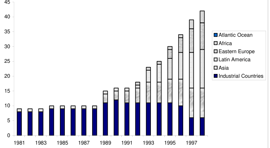
The agency ratings we employ are those of Standard and Poor’s. The rating histories provided by rating agencies for most sovereigns are relatively short, especially for subinvestment grade sovereign issuers. Figure 1 shows the sovereigns rated by Standard and Poor’s in the period 1981 to 1998 broken down by region. Since almost all industrial countries have A-grade ratings, it is apparent from the figure that only since the mid-1990s have significant numbers of sub-investment grade sovereigns been rated.
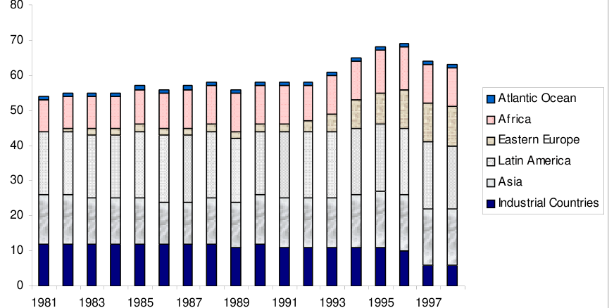
The internal bank ratings data we use comes from a large bank that systematically rated a large group of sovereign borrowers over a twenty-two-year period. The breakdown by year and by region is shown in Figure 2. The unusual feature of the data is the length of the time series since most data on internal bank ratings spans only a very short and recent period of time.
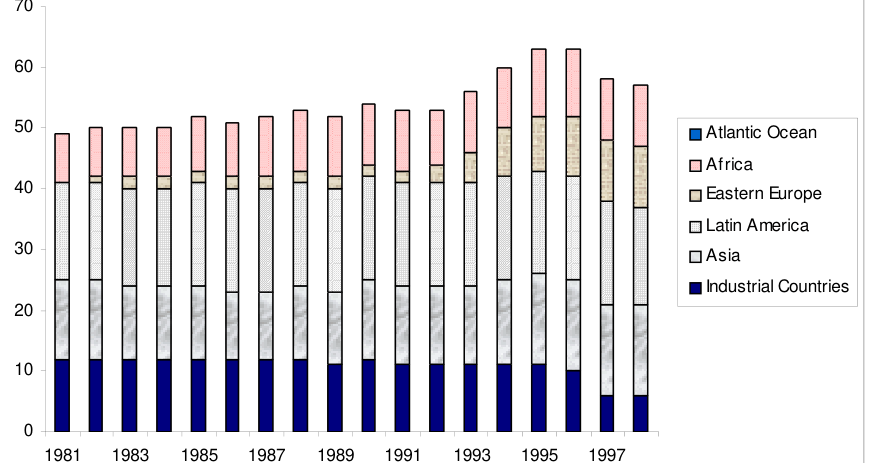
Lastly, the quantitative ratings series we employ are derived from an econometric model of sovereign credit quality, estimated from macroeconomic and financial data. The techniques involved in implementing this model are described in Section 2 below; but, in brief, a probit model is used to estimate sovereign defaults over the period 1981 to 1998. Standard and Poor’s ratings data is used to benchmark the model so that it produces ratings histories comparable in meaning to Standard and Poor’s ratings.
The main exercise we perform on these ratings is to examine whether current ratings according to one ratings system can be used to forecast downgrades or upgrades of another over the following one-year period. While this does not show that one ratings system is better at forecasting defaults than another (to establish this would require large amounts of default data), it does show that one set of ratings is more timely than another in the information it conveys.
Our main finding is that downgrades in agency ratings and internal bank ratings are predictable using the quantitative ratings produced by our econometric model. On the other hand neither of the judgmental ratings systems has predictive power either against the other or for the quantitative ratings. Upgrades in the quantitative ratings are predictable using the judgmental ratings.
Our findings may be compared to the conclusions of Delianedis and Geske (1998) who suggests that negative changes in corporate agency ratings may be forecast well in advance using equity data.
The structure of our paper is as follows. Section 2 described the methods we employ to derive quantitative ratings from an econometric model. Section 3 presents nonparametric and parametric tests of the predictability of the three sets of ratings. Section 4 concludes.
2. An Econometric Model of Quantitative Ratings
2.1 Methodology
In this section, we describe in greater detail the approach we take to estimating quantitative ratings for sovereigns. Hu, Kiesel and Perraudin (2002) employed similar techniques in studying rating transition matrices. That paper, however, did not focus on the levels of ratings implied by this approach or how their informational content compares with that of agency and internal bank ratings.
The basic idea is to model default/non-default event using a probit model and publicly available macroeconomic and financial variables. It is assumed that
R = β' X +ε (1)
Here, X is a column vector of predetermined variables, β is a row vector of parameters and ε is assumed to have a standard normal distribution. Default occurs if R<0. Under these assumptions, the likelihood for a sovereign in a particular year is
Φ − β' X ⎧ Prob(default) = ( ) (2) ⎨ 1− Φ − β' X Prob(no default) = ( ) ⎩
The parameters in the row vector β may be estimated using standard Maximum Likelihood methods and then the index β X provides a measure of the credit quality of the country in question in a particular year.
To produce ratings, one must map the index of credit quality implied by the model, β X, into a set of discrete ratings categories. The most obvious approach is to assign different ratings to different ranges for the fitted credit quality index βML X . (Here, the subscript ML indicates that the parameters are the Maximum Likelihood estimates.) Different approaches may be devised to determining the ranges. The approach we take is to benchmark the model off Standard and Poor’s ratings by estimating an ordered probit model of ratings j=0,1,..,J where 0 denoted the default state and J indicates the highest rating category. The rating in a given year is assumed again to depend on the variable R in that the rating j is given by j = 0 if R ≤ 0 ⎧ j = 1 if0 < R ≤ Z ⎪[2] (3) ⎨ M M ⎪ ⎪⎩ j = J +1 if ZJ ≤ R
for a set of scalar cut-off points Zk where 0 < Z[1]<…< ZJ.
Estimation then involves determining the vector of macroeconomic-financial parameters β and the cut-off points Zk. One can either estimate the model sequentially, first, estimating the β parameters from default-non-default observations and then using the rating observations to pin down the cut-off points. We prefer to estimate the two sets of parameters simultaneously, however This involves formulating a likelihood using terms as in equation (2) for years in which the country in question is not rated by standard and Poor’s and using ordered-probit terms of the kind:
' X ⎧ Prob( j = 0) = Φ(−β ) Φ Z −β' X Prob( j = )1 = ( ) ⎪[1] (4) ⎨ = M M ⎪ ⎪⎩Prob( j = J +)1=1− Φ(ZJ −β' X )
for years in which the country in question is rated.[1]
Once estimates of the model parameters, the Z’s and the β’s, have been obtained, one may predict the rating for each sovereign and each year in the sample by calculating the index β' Xkt (where k indicates a particular sovereign and t the time period) and determining the interval [Zj-1,Zj] into which the index falls. Thus, one may create rating histories for all the countries and all periods for which the requisite macroeconomic and financial variables are available.
2.3 Data Employed in the Estimation of Quantitative Ratings
We employ default-non-default data provided by the UK’s export credit insurer, the Export Credit Guarantee Department (ECGD). This provides a consistent measure of default from 1981 to 1998. (Using a default definition based on public bond defaults is not possible over this period since almost none of the countries that defaulted on liabilities in the 1980s had issued bonds.)
The explanatory variables in our model are variables that one may judge, on a priori grounds, are likely to influence credit standing. We also examined past empirical studies in order to inform our choice of variables. Relevant past research includes econometric studies of (i) sovereign ratings (see Cantor and Packer (1996), Haque, Kumar, Mark and Mathieson (1996), Juttner and McCarthy (1998), Monfort and Mulder (2000)), (ii) sovereign defaults (see Edwards (1984)), and (iii) spreads on sovereign debt (see Burton and Inoue (1985), Edwards (1986), Cantor and Packer (1996), Eichengreen and Mody (1998), Min (1998), Kamin and Kleist (1999)).
The most general set of variables we included is:
1. A dummy variable that is unity if the country was in default in the previous year and zero otherwise.
2. The ratio of debt service to exports.
3. The ratio of debt to GNP.
4. The ratio of reserves to debt.
5. The ratio of reserves to imports.
6. Inflation.
7. GNP growth.
8. The ratio of the current account balance to GNP.
9. A dummy that is unity if the country is a non-industrial country and zero otherwise.
Variables that were likely to change significantly over time, namely inflation GNP growth and the ratio of the current account balance to GNP were also included lagged one year. While other variables may always be included, we were keen not to experiment with different specifications since this might lead to over-fitting and reduce the out-of-sample forecasting power of our estimated model. Having estimated the model with the full range of variables, we eliminated variables with insignificant tstatistics and used the resulting model as our benchmark model for other calculations.
2.4 Estimates of the ordered probit model of ratings and default
Table 1 shows the estimates of the ordered probit model of ratings and default events. The parameters appear reasonably stable between the general and the restricted model, suggesting that there is no major issue of multicolinearity. Default is associated with low values of the index β X so negative parameter values imply variables are negatively associated with credit quality. The signs of the parameters shown in Table 1 are all intuitively sensible. Being in default the year before and having high debt to export and debt to GNP ratios and having high current or lagged inflation rates are associated with lower credit quality. Having high reserves to debt or reserves to imports, high GNP growth or a high ratio of current account surplus to GNP are all associated with high credit quality. The cut-off point parameters are not very informative as they are parameterised in the model as the square root of gaps between successive rating cut-off points. To economise on space, we do not report them.
3. Predictability
3.1 Non-Parametric Tests of Predictability
Figures 4 and 5 show the results of nonparametric tests of predictability of each set of ratings for the other sets. The approach we take resembles that employed by Kealhoffer
(2001) in his comparison of the informational content of Moody’s ratings and a Merton-style equity-based model of default prediction. The analysis uses observations of countrys’ ratings at the start of July each year for which ratings are available. Observations are placed into buckets according to their ratings as measured by one rating system, rating system i. The observations within each bucket are then ranked according to their rating based on another rating system, rating system j, and divided into quintiles.
If rating system j contains no information about credit quality over and above the information in the system i rating, then one may expect that observations in the different quintiles will not exhibit very different future behavior. In particular, observations in the quintiles associated with the lowest (highest) system j ratings should not show significantly larger numbers of downgrades (upgrades) than those not in these quintiles.
Figures 4 and 5 show the numbers of observations in each quintile for different combinations of system i and system j ratings. Figure 4 focuses on numbers of upgrades in the system i ratings over the following year while Figure 5 looks at numbers of downgrades in system i ratings over the following year. To take an example, in the upper left-hand histogram in Figure 4, the horizontal axis shows system j quintiles for quantitative ratings while the vertical axis shows the number of downgrades within the following year in Standard and Poor’s ratings, Standard and Poor’s being in this case system i. In all the plots, the leftmost quintile corresponds to the 20% of observations that have the highest system j ratings while the rightmost quintile corresponds to observations with the lowest system j ratings.
The figures suggest that the Standard and Poor’s ratings and the bank ratings may possibly have some predictive power for upgrades in the quantitative ratings but that there are strong indications that quantitative ratings have power to predict downgrades in the other systems’ ratings.
To test these conclusions statistically, we calculated the probabilities of observing the numbers of upgrades and downgrades recorded in Figures 4 and 5 given the null hypothesis that the observations of upgrades or downgrades are uniformly distributed across the system j ratings quintiles. The probabilities were calculated using a Monte Carlo with the appropriate numbers of observations. Table 2 shows the results of these calculations.
As one may see from the upgrade part of Table 2, the probabilities of observing the quantitative ratings upgrades in the data given under the null that they are uniformly distributed across the Standard and Poor’s and bank rating quintiles are 2.2% and 17.3%, respectively. The downgrade part of Table 2 shows that the probabilities of observing the number of downgrades in Standard and Poor’s and bank ratings given that they are uniformly distributed across the quantitative rating quintiles is 1.1% and less than 0.1%, respectively.
3.2 Multivariate Tests of Predictability
We also estimated a multivariate probit model to assess the probability of ratings changes in one rating system using the information in both the other ratings systems as explanatory variables. To be precise, we use a binary variable
Y = 1, if there is an upgrade (downgrade) within 1 year for the evaluated rating system, Y=0, otherwise.
We then assume there is a linear index such that
Y = 1 if β[0] + β[1]D[1] + β[2]D[2] +ε> 0 and Y = 0 otherwise. We assume that the ε are normally distributed and that
Dn = 1, if the nth explanatory rating system (where n=1,2) is higher (lower) than the evaluated one Dn =0, otherwise
The results are reported in Table 3. The coefficients generally have the expected sign. The results tend to confirm the non-parametric test results in that quantitative ratings are shown to have significant predictive power for future downgrades in Standard and Poor’s ratings and bank ratings, whereas Standard and Poor’s ratings are useful in predicting upgrades in quantitative and bank ratings. Standard and Poor’s ratings are also very significant for downgrades in bank ratings.
4. Conclusion
The picture that emerges from our study is one in which the different rating systems (especially the Standard and Poor’s and quantitative ratings) have significant explanatory power for changes in the ratings produced by other systems. Some degree of predictability is to be expected given that rating categories are discrete. If underlying credit quality is continuous and the ranges of credit quality corresponding to the discrete categories in each rating system do not precisely coincide, the ratings supplied by the different systems may differ without there being inconsistencies and there may be predictability.
Nevertheless, several strong findings emerge. In particular, the non-parametric results show graphically that a very large fraction of downgrades in the judgmental variables correspond to observations with relatively low quantitative ratings. By this measure, Standard and Poor’s ratings also appear to have substantial explanatory power for upgrades in quantitative ratings. The multivariate probit results broadly confirm these findings.
References
Basel Committee on Banking Supervision (1999), ‘A new capital adequacy framework: consultative paper’, June.
Basel Committee on Banking Supervision (2001), ‘ The new Basel Accord: consultative package’, January.
Berkowitz, J. (2001) “Testing Density Forecasts with Applications to Risk Management” Journal of Business & Economic Statistics 19, 465—474.
Burton, F.N. and H. Inoue, (1985) “The Influence of Country Factors on the interest differentials on International Lendings to Sovereign Borrowers,” Applied Economics, 17, 491-507.
Cantor, R. and F. Packer, (1996) “Determinants and Inputs of Sovereign Credit Ratings,” FRBNY Economic Policy Review, 2(2), 37-53.
Delianedis, G. and R. Geske, (1998) “Credit Risk and Risk Neutral Default Probabilities: Information about Ratings Migrations and Defaults,” working paper Anderson School, UCLA, Los Angeles.
Edwards, S., (1986) “The Pricing of Bonds and Bank Loans in International Markets,” European Economic Review, 30, 565-89.
Edwards, S., (1984) “LDC Foreign Borrowing and Default Risk: An Empirical Default Risk, 1976-1980,” American Economic Review, 74, 726-34.
Eichengreen, B. and A. Mody, (1998) “What Explains Changing Spreads on Emerging Market Debt? Fundamentals or Market Sentiment?” NBER Working Paper, No.6408.
Frerichs, H. and Löffler, G. (2002) Evaluating Credit Risk Models: A Critique and A Proposal, Preprint, University of Frankfurt.
Greene, W. H., (1997) Econometric Analysis, Prentice Hall, 3rd edition.
Haque, N.U., M. Kumar, N. Mark, and D. Mathieson, (1996) “The Economic Contents of Indicators of Developing Country Creditworthiness,” IMF Staff Papers, 43(4), 688- 724.
Juttner, J.D. and J. McCarthy, (1998): “Modelling a Rating Crisis”, Macquarie University, Sydney, unpublished.
Kamin, S. and K. Kleist, (1999) “The Evolution and Determinants of Emerging Market Credit Spreads in the 1990s,” BIS Working Paper.
Lopez, J.A. and Saidenberg, M.R. (2000) “Evaluating Credit Risk Models, Journal of Banking and Finance, 24(1-2), 151-165.
Min, H. (1998), “Determinants of emerging market bond spreads: Do economic fundamentals matter?” World Bank working paper.
Monfort, B. and C. Mulder, (2000) “Using Credit Ratings for Capital Requirement on Lending to Emerging Market Economies: Possible Impact of Basel Accord.”, IMF Working Paper, March.
Treacy, William F. and Mark Carey, (2000) “Credit Risk Rating Systems at Large U.S. Banks,” Journal of Banking and Finance, 24 (1-2) 167-201.
| Parameters | Estimates | t-statistics | Estimates | t-statistics | |
|---|---|---|---|---|---|
| Constant | 0.80 | 5.62 | 1.39 | 10.12 | |
| Previous year | default dummy | -2.78 | -10.23 | -2.60 | -9.91 |
| Debt service | to Exports | -0.65 | -0.89 | -- | -- |
| Debt to GNP | -1.30 | -3.29 | -1.92 | -5.16 | |
| Reserves to | Debt | 1.95 | 3.91 | 1.75 | 6.24 |
| Reserves to | Imports | 3.68 | 1.05 | -- | -- |
| Inflation | -1.57 | -2.76 | -1.64 | -3.01 | |
| GNP growth | 1.85 | 2.35 | 1.56 | 2.12 | |
| Current Balance | to GNP | 0.40 | 0.17 | -- | -- |
| Dummies for | non-industrial countries | -3.57 | -8.28 | -3.35 | -12.25 |
| Lagged Inflation | -0.95 | -2.59 | -0.99 | -3.05 | |
| Lagged GNP | growth | 1.65 | 1.94 | -- | -- |
| Lagged Current | Balance to GNP | 0.77 | 0.34 | -- | -- |
| Average log | likelihood | -12.60 | -- | -11.56 | -- |
| Number of | cases | 896 | -- | 1078 | -- |
| Evaluated | Predicting Rating | changes Observations | in the tail | P-Value |
|---|---|---|---|---|
| S&P | Quantitative | 16 | 1 | 0.973 |
| Bank | Quantitative | 49 | 13 | 0.168 |
| Bank | S&P | 49 | 14 | 0.098 |
| Quantitative | S&P | 122 | 34 | 0.022 |
| Quantitative | Bank | 122 | 29 | 0.173 |
| S&P | Bank | 16 | 5 | 0.203 |
| DOWNGRADES | ||||
| Evaluated | Predicting Rating | changes Observations | in the tail | P-Value |
| S&P | Quantitative | 17 | 8 | 0.011 |
| Bank | Quantitative | 55 | 26 | 0.000 |
| Bank | S&P | 55 | 17 | 0.037 |
| Quantitative | S&P | 138 | 25 | 0.742 |
| Quantitative | Bank | 138 | 21 | 0.940 |
| S&P | Bank | 17 | 5 | 0.243 |
| UPGRADES | |||
|---|---|---|---|
| S&P | Constant | Quantitative | Bank |
| Estimates | -2.130 | 0.596 | -2.070 |
| t-statistics | -10.690 | 1.716 | -7.937 |
| Marginal prob. Changes | -- | 0.046 | -0.024 |
| BANK | Constant | Quantitative | S&P |
| Estimates | -2.336 | 0.051 | 1.132 |
| t-statistics | -8.210 | 0.184 | 3.708 |
| Marginal prob. Changes | -- | 0.004 | 0.107 |
| QUANTITATIVE | Constant | S&P | Bank |
| Estimates | -1.995 | 1.106 | 0.161 |
| t-statistics | -10.688 | 3.343 | 0.476 |
| Marginal prob. Changes | -- | 0.170 | 0.019 |
| DOWNGRADES | |||
| S&P | Constant | Quantitative | Bank |
| Estimates | -2.488 | 1.138 | 0.434 |
| t-statistics | -7.352 | 3.838 | 1.560 |
| Marginal prob. Changes | --- | 0.106 | 0.033 |
| BANK | Constant | Quantitative | S&P |
| Estimates | -1.965 | 0.732 | 5.804 |
| t-statistics | -11.418 | 2.436 | 19.93 |
| Marginal prob. Changes | --- | 0.083 | 0.961 |
| QUANTITATIVE | Constant | S&P | Bank |
| Estimates | -1.489 | 0.080 | 0.271 |
| t-statistics | -10.767 | 0.230 | 0.959 |
| Marginal prob. Changes | --- | 0.013 | 0.044 |
Notes
[1] For more details on the ordered probit, see Green (1997), §19.8.